Does Car-Sharing Reduce Car-Use? An Impact Evaluation of Car-Sharing in Flanders, Belgium

Abstract

Private car-use is a major contributor of greenhouse gases. Car-sharing is often hypothesised as a potential solution to reduce car-ownership, which can lead to car-sharing users reducing their car-use. However, there is a risk that car-sharing may also increase car-use amongst some users. Existing studies on the impacts of car-sharing on car-use are often based on estimates of the users’ own judgement of the effects; few studies make use of quasi-experimental methods. In this paper, the impact of car-sharing on car-ownership and car-use in Flanders, Belgium is estimated using survey data from both sharers and non-sharers. The impact on car-use is estimated using zero-inflated negative binomial regression, applied to matched samples of car-sharing users and non-users. The results show that the car-sharing may reduce car-use, but only if a significant number of users reduce their car-ownership. Policy intervention may therefore be required to ensure car-sharing leads to a reduction in car-use by, for example, discouraging car-ownership. Further research using quasi-experimental methods is required to illuminate whether the promise of car-sharing is reflected in reality.

1. Introduction

Cars are a major contributor to greenhouse gas (GHG) emissions, representing 14% of the world’s GHG emissions in 2010 [1]. Car-sharing is believed to be a potential solution that could induce behavioural changes through a reduction in car-ownership and of car-use. In addition, car-sharing may support the development of cars with higher fuel efficiencies and much longer functional lifetimes (in terms of distance travelled), leading to fewer cars being produced [2]. Thus, through both behavioural changes from drivers and changes to the cars themselves, car-sharing may reduce impacts associated both with car production and with car-use. There has been some empirical evidence of environmental benefits: Martin and Shaheen [3] estimated a reduction in GHG emissions due to a reduction in car-ownership and car-use, while Chen and Kockelman [4], using life-cycle analysis, estimated a reduction of approximately 51% in emissions of car-sharing users, with reductions in car-use the major contributor. Amatuni et al. [5] re-estimated the impacts of other analyses using a life-cycle approach, and found that, due to overestimates of the functional lifetime of shared cars, the benefits of car-sharing may have been overestimated; nonetheless, car-sharing still resulted in a (small) reduction in GHG emissions. In contrast, a prospective study of potential car-sharing members in Korea, Jung and Koo [6] found that car-sharing may lead to an increase in GHG emissions due to an increase in car-use amongst some users. The importance of changes to car-ownership and car-use, then, are central to the realisation of environmental benefits. While the majority of existing studies have generally found a reduction in both car-ownership and car-use amongst car-sharing users, most of these studies are based on directly asking users how their behaviour has changed, rather than using methods more appropriate for quantitative impact evaluation, that is, quasi-experimental methods. In this study, we complement the existing literature by estimating the impact of car-sharing on car-use using a quasi-experimental approach, and in doing so, highlight the sensitivity of car-use impacts to car-ownership impacts. We draw some implications for policymakers, while for researchers, we discuss some key methodological issues in measuring the impacts of car-sharing, and recommend solutions.

In the following section, a summary of findings of existing car-sharing impact studies is presented and their methodological approach reviewed. In Section 2, we describe the data and method used in this study. Section 3 contains the results of the survey and analysis, and Section 4 draws out the main findings from this research. Section 5 concludes.

1.1. Existing Car-Sharing Impact Studies

There have been a number of studies that investigate the impacts of car-sharing on car-ownership and car-use, a selection of which are summarised in

Table 1. Impact on car-ownership found in other studies.

Authors	Results	Method of Inference
6T-Bureau De Recherche [7]	Round-trip car-sharing reduced the number of private cars by 32% (Paris)	Self-assessed
Becker et al. [8]	6% of free-floating car-sharing households gave up a car (Basel, Switzerland)	Quasi-experimental: Difference-in-difference and panel regressions with control group
Cervero et al. [9]	Round-trip car-sharing households were 12% more likely to give up a car compared to non-members (San Francisco, USA)	Quasi-experimental: regressions with control group
Firnkorn and Müller [10]	Between 4.7% and 11.4% of free-floating car-sharing users have one fewer car because of car-sharing (Ulm, Germany)	Self-assessed
Giesel and Nobis [11]	13.6% of free-floating car-sharing users and 23.6% of round-trip car-sharing users either have or plan to shed a car (Germany)	Self-assessed
Martin et al. [12]	Car-sharing users reduce their cars owned by 0.23 cars, on average, compared to before their joined car-sharing (North America)	Self-assessed and filtering
Mishra et al. [13]	Car-sharing households have 0.17 fewer cars on average because of car-sharing (California)	Quasi-experimental: Propensity score matching and structural equation model with control group
Nijland and van Meerkerk [14]	17% of users got rid of a car; a further 23% of users did not buy a car (Netherlands)	Self-assessed and filtering
Wu et al. [15]	32% of users round-trip reduced their car-ownership after joining car-sharing (London, UK)	Simple before–after difference
Le Vine and Polak [16]	37% of free-floating users reported car-sharing caused them to own fewer cars (London, UK)	Self-assessed
Kim et al. [17]	31% (2014) and 32% (2018) of users discarded, will discard, or postponed the purchase of a car (Seoul, Korea)	Self-assessed

and

Table 2. Impact on car-use found in other literature.

Authors	Results	Method of Inference
6T-Bureau De Recherche [7]	45% reduction in km driven per month (Paris, France)	Self-assessed
Becker et al. [18]	38% of users reduced car usage frequency; 16% of users increased car usage frequency (Switzerland)	None
Cervero et al. [9]	Reduction of 7.1 vehicle miles (11.4 km) travelled per use per day (San Francisco, USA)	Quasi-experimental: regressions with control group
Martin and Shaheen [3]	Average 43% reduction in km travelled by car across five different cities (USA and Canada)	Self-assessed and filtering
Martin and Shaheen [19]	Car-sharing users reduced their miles travelled in cars by 11% on average, across five different cities (USA and Canada)	Self-assessed and filtering
Nijland and van Meerkerk [14]	Average 1750 km reduction in km travelled by car per member per year (Netherlands)	Self-assessed and filtering
Wu et al. [15]	Round-tip car-sharing users reduce vehicle miles travelled by 564 miles (902 km) per user per year (London, UK)	Self-assessed

. The main criteria for selection was that studies should be ex-post evaluations, i.e., estimating actual changes in car-ownership or car-use that have occurred, as opposed to ex-ante predictions. For the purposes of this study, car-sharing is defined as the use of cars, parked on-street, by different users who may not own (or co-own) the car. Following existing distinctions in the car-sharing literature, traditional car-rental, as well as ride-sharing or car-pooling are out-with the boundaries of this study since they are conceptually different to car-sharing – car-sharing attempts to replace the feeling of owning a car, which car-pooling or ride-sharing does not offer (one does not drive the car), and neither does car-rental (cars are generally not provided at short notice and/or in close proximity to one’s home). Car-sharing can be provided through a company that owns a fleet of cars and shares them for members to use (b2c car-sharing). Cars owned by members of the public can also be shared either amongst neighbours or on a platform where it is open to all users (p2p car-sharing). Round-trip car-sharing describes a shared car starting and ending its journey from the same location, as opposed to free-floating car-sharing, where the rental period of a shared car does not have to start and end at the same place.

An initial search for literature was conducted with Scopus (http://www.scopus.com); additional studies were found through references. A consistent finding among these studies is that a significant number of car-sharing users reduce the number of cars they own, either because they sell or scrap a car, or because they do not purchase a car they otherwise would have bought. Similarly, all studies in Table 2 find that car-sharing users reduce their car-use, on average; some studies explain this by observing that car-sharers who have fewer cars because of car-sharing reduce their car-use, while those whose car-ownership is not affected increase their car-use [3,14,15]. The impact among the former group is normally larger than the latter group; in other words, users who have fewer cars reduce their car-use by more than the users whose car-ownership is not affected increase their car-use.

1.2. Review of Methods

In impact evaluation, a crucial part of the analysis is to estimate the counterfactual, which is the outcome that would have occurred if the intervention (in this case car-sharing) had not occurred. However, estimating the counterfactual is difficult because it is unobservable—there is no parallel universe where we can observe what would have happened had the intervention not occurred. Instead, different methods are used to estimate this counterfactual, the appropriateness of which can be determined by their internal validity (i.e., the extent to which they are free from bias). A randomised experiment is generally considered the most internally valid method to estimate a counterfactual [20] (p. 64), where a random group of individuals (the treatment group) are exposed to a treatment (e.g., a new policy, or in this case, car-sharing) while a statistically similar group of individuals serve as a comparison group (the control group). The average difference in the outcomes of interest is known as the average treatment effect. However, in many settings, experiments are not possible and thus survey data is used instead (known as observational studies). Observational studies differ from experiments since the survey respondents are not randomly assigned to receive a treatment: instead, respondents choose to receive the treatment (e.g., joining car-sharing) based on their own unique circumstances, making impact assessments vulnerable to selection bias. In such cases, statistical methods, collectively known as “quasi-experimental” methods, are used to try to replicate the conditions of an experiment to estimate the causal impact of a treatment with as little bias as possible [20].

Despite the strong foundations of quasi-experimental methods, in most of the studies reviewed in Table 1 and Table 2, car-sharing users are asked to estimate their own counterfactual, either in retrospect or hypothetically (labelled “self-assessed” in Table 1 and Table 2). This is sometimes combined with filtering out users who are suspected to have changed their behaviour for other reasons (e.g., moving house). Since neither self-assessment or filtering methods mimic a randomised experiment, they are not quasi-experimental. For example, Martin and Shaheen [3] estimate the change in km driven for two different types of user: first, for users who gave up a car, the change in impact was measured based on each user’s estimate of how far they travelled by car in the year previous to joining car-sharing; second, for users who say they would have bought a car, users were asked how far they would travel in the car they would have bought. Although these studies make the most of the data collected, there are issues. The internal validity of a self-assessed counterfactual relies on respondents being able to correctly estimate their own potential behaviour and correctly attributing this change to car-sharing and not other confounding factors. However, in impact evaluation literature, self-assessment is rarely used or recommended due to various cognitive biases that cause respondents to over or underestimate their own counterfactual [21,22,23]. Quasi-experimental methods, in contrast, remove the issue of cognitive biases resulting from self-assessed counterfactuals and can control for confounding factors (that is not to say that quasi-experimental methods are sure to be internally valid—they also introduce other sources of bias, see Section 2.5.2). However, far fewer car-sharing impact studies make use of a quasi-experimental approach (i.e., References [8,9,13]). Of these, only Cervero et al. [9] estimate changes in car-use caused by car-sharing. The lack of quasi-experimental studies may be partly due to the amount of data required—a control group of non-users is a minimum requirement, with the most robust methods additionally requiring longitudinal data.

A further issue with car-sharing impact studies to-date is that they neglect the sensitivity of car-use impacts to the effect car-sharing has on car-ownership. As will be discussed in more detail in Section 2.3, over/under estimating the impact of car-sharing on car-ownership can lead to an over/under estimate of the impact on car-use. To identify the causal impact of car-sharing on car-ownership and car-use requires a method to identify the direction of causality (someone may be car-less because they join car-sharing, or vice-versa). This is challenging in observational studies, which may explain why self-assessed counterfactuals are popular. However, this inherent uncertainty in the estimation of car-ownership effects is rarely accounted for when estimating the impact on car-use.

In summary, the impact of car-sharing on both car-ownership and car-use has most often been estimated using self-assessed counterfactuals, with very few studies using quasi-experimental methods. In particular, to our knowledge only one study to date has used a quasi-experimental approach to estimate the impact of car-sharing on car-use (i.e., Cervero et al. [9]). In this study, we add to the literature by using a quasi-experimental method to estimate the impact of car-sharing on car-use. Furthermore, the sensitivity of car-use impacts to the car-ownership effect is captured and documented.

2. Materials and Method

2.1. Survey Design

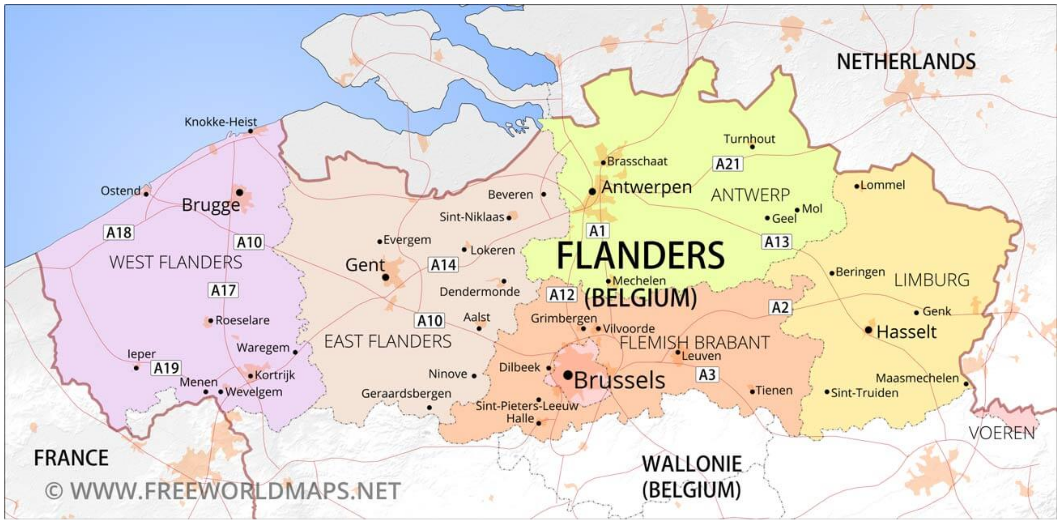
Flanders is the Dutch speaking region in Belgium with a total population of 6.6 million and a population density of 487 inhabitants per km${}^2$ [24]. The major Flemish cities are Antwerp, Ghent, and Bruges, while Flanders also borders the Belgian capital, Brussels (Figure 1). A report from 2019 found that there are approximately 75,000 car-sharing users in Flanders and a further 104,000 in the neighbouring Brussels Capital region [25]. Car-sharing firms are present in all of Flanders’ major cities and include round-trip, free-floating, and p2p systems. However, to the authors’ knowledge, there have been no studies that research the impact of car-sharing on car-use in Flanders. To estimate this impact, an online survey in Dutch (some Dutch speaking residents of Brussels also completed the survey) was launched on the 31st of August 2018 and accessible until the 12th of November 2018. Links to the survey were spread through newsletters, the mailing lists of environmental and mobility organisations, social media and local governments. The survey covered two research objectives, namely the impact of car-sharing on behaviour (this study), and the identification of barriers for consumers to join car-sharing (forthcoming). The survey consisted of four parts. In the first part, respondents were asked about personal and household characteristics, such as age, education, employment, household composition, number of cars, attitudes and so forth. In the second part, respondents were asked about their current personal travel behaviour in a typical week; additionally, car-sharing users were asked about the impact of car-sharing on their travel behaviour. A typical week was chosen, as opposed to a specific week, since the survey was answered at random, at different times, which increases the risk that time-related factors, such as holidays or rare work trips, may bias results. The focus of the third part was a discrete choice experiment (DCE) that gave non-users a choice between buying a car or joining car-sharing, while car-sharing users were asked to choose between two different car-sharing systems. Finally, the fourth part consisted of a number of questions on attitudes towards car-sharing and users’ experiences of it.

Because of its design, the sample is not representative, but was instead intended to reach as many car-sharing users as possible. A truly random sample would require a total response of approximately 20,031 respondents to match the number of car-sharing users reached in this survey (228). (Based on 75,000 Car-sharing users in Flanders, and a population of 6.6million [24], the percentage of car-sharing users in Flanders is approximately 1.1%, therefore, to reach 228 car-sharing users in a random sample would require approximately 20,031 respondents.) By spreading the survey through Flemish and Belgian car-sharing organisations, we hoped to record a significant number of observations of car-sharing users. However, some car-sharing organisations refused to do so, leading to an over-representation of those who did agree, in particular the p2p organisation Degage. As a result, the sample is not representative of different car-sharing organisations. However, we have adjusted for this sampling bias to some extent by estimating the effect for p2p users separately.

2.2. Rubin Potential Outcome Framework

The basis for causal inference in this study is the Rubin potential outcome (PO) framework, for which the estimation of the counterfactual is crucial [27]. In this study, the counterfactual is the behavioural outcome (number of cars owned and km driven by car) of a car-sharing user that would have happened if they were not a member of car-sharing. The difference between the observed outcome and the estimated counterfactual gives the treatment effect.

Two assumptions are crucial for causal inference in quasi-experimental methods under the PO framework: the stable unit treatment value assumption (SUTVA) and unconfoundedness. The former assumes that those who receive the treatment (e.g., car-sharing) do not affect the outcomes of others, and that each unit receives the same treatment [27] (p. 10). Unconfoundedness requires that the outcome does not affect the treatment [27] (p. 258). Both of these will be discussed further below.

2.3. Conceptual Framework

The goal of this study is estimate the impact of car-sharing on car-use. This estimation is, however, complicated by the relationship between the impact of car-sharing on car-ownership since the number of cars a person owns affects how much he/she will use a car. For example, the introduction of car-sharing to one’s neighbourhood may cause an inhabitant to join car-sharing and to sell his/her car (or one of the cars in the household), reducing the user’s access to private cars. This change in access (from having one private car fewer but having access to car-sharing) is likely to reduce how much he/she drives. In contrast, an inhabitant who does not have a car (and had no plans to buy one, thus his/her car-ownership is unaffected by the introduction of car-sharing) will increase his/her access to cars by joining car-sharing, which can lead to an increase in car-use. This relationship has been uncovered empirically in other studies, such as Martin and Shaheen [3] and Wu et al. [15], and is also discussed by Jung and Koo [6] and Ke et al. [28]. These hypothetical examples show that it is crucial to first establish the effect on car-ownership before estimating the effect on car-use. To ignore it introduces a risk of bias: if all users without a car are assumed to have gotten rid of a car because of car-sharing, then the impact of car-sharing on car-ownership would be overestimated, thus also affecting the estimated impact on car-use. In order to gain a better understanding of this effect, we have assessed the sensitivity of the car-ownership effect on car-use—see Section 2.4.

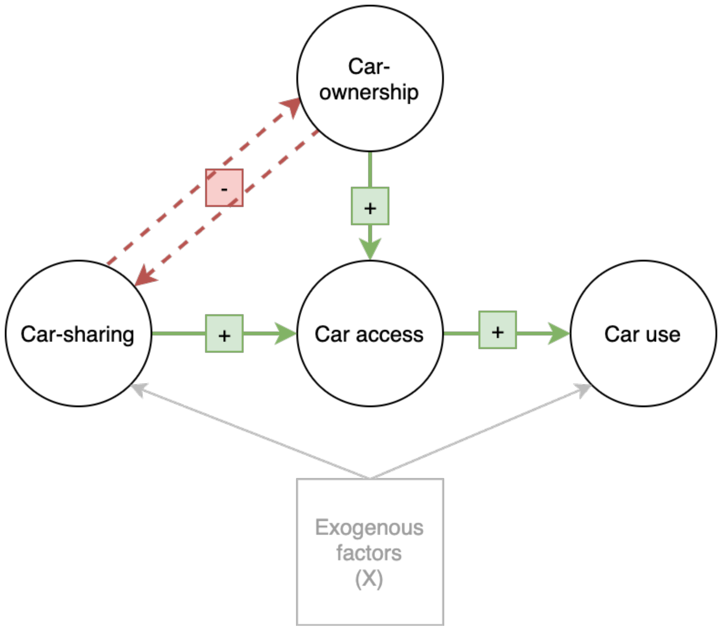
The relationship between car-sharing and these outcomes is summarised in the causal loop diagram (Figure 2). The two dashed arrows represent the different relationships between car-sharing and car-ownership. They are negative since an increase in one causes a decrease in the other: joining car-sharing causes a decrease in cars owned (first example above), or lower car-ownership increases the likelihood of joining car-sharing (second example). According to the diagram, there is both a direct and an indirect effect of car-sharing on car-use. The direct effect is that, all else being equal, joining car-sharing leads to higher access to cars, which leads to more car-use (represented by the positive arrow from car-sharing to car access to car-use). The indirect effect is the result of the effect of car-sharing on car-ownership: car-sharing reduces car-ownership, which reduces car access, and finally reduces car-use. If there is no effect of car-sharing on car-ownership, then there is no indirect effect. Based on this framework, we can consider two groups: lower access users (LAUs) and higher access users (HAUs). LAUs are those who have one fewer car because of car-sharing, and thus experience both a direct and indirect effect on car-use. HAUs, however, experience only the direct effect of car-sharing, since their car-ownership is not affected.

Table 3. The relationship between the effect of car-sharing on car-ownership and car-use.

Group	Effect on Car-Ownership	Effect on Car-Use
Lower access users (LAUs)	Car-sharing causes users to have less cars	Increase in car-use (direct effect); Decrease in car-use (indirect effect)
Higher access users (HAUs)	No effect	Increase in car-use (direct effect only)

summarises these relationships.

The mutually-causal relationship between car-sharing and car-ownership makes the counterfactual outcomes (both car-ownership and car-use) challenging to estimate in most observational studies since it is very difficult to establish this direction of causality from simply observing changes in outcomes. Other car-sharing studies that use a quasi-experimental approach, such as Cervero et al. [9] and Becker et al. [8], make use of longitudinal data, while Mishra et al. [13] uses an instrumental variable approach. Our data is cross-sectional, however, with no valid instrument. Thus, to overcome this identification problem in our survey, we have used a self-assessed counterfactual. We are therefore able to untangle the mutually causal relationship into two dichotomous relationships (grouped into LAUs and HAUs), allowing us to estimate the impact on car-use with less bias.

In addition to the relationship between outcomes, there are a number of exogenous factors that both determine whether someone joins car-sharing, and their car-use, represented in Figure 2 by the grey box. These factors may include, for example, where a user lives. Such factors are controlled for in the calculation of the impact of car-sharing to ensure unconfoundedness—more on this in the Section 2.5.2.

Table 4. Overview of method used in this study.

Effect Estimated	Methodological Issue	Solution
Car-ownership	Reverse causality—how to distinguish between users who have fewer cars because of car-sharing and those who join car-sharing because they own fewer cars	Self-assessed counterfactual sensitive to the strength of causality (Section 2.4)
Car-use (HAUs)	Estimation of counterfactual private car-use for users with at least one private car	Self-assessed counterfactual based on hypothetical question (Section 2.5.1)
Car-use (LAUs)	Threat to unconfoundedness due to omitted variable bias—systematic differences between car-sharing users and non-users	Pre-screening of control group to only contain non-users interested in joining car-sharing (Section 2.5.2)
	Lack of overlap [29]—there are car-sharing users for whom there is no adequate comparison amongst non-users	Use nearest neighbour propensity score matching to estimate more robust model with most similar observations (Section 2.5.2 and Section 3.3)
	Threat to unconfoundedness due to Lack of balance [29]—adjusting for the influence of other factors that might affect both the decision to join car-sharing and car-use	Regression analysis using zero inflated negative binomial models (Section 2.5.3 and Section 3.4)

summarises the different effects, the methodological challenges they present, and the solution used in this study. It shows that quasi-experimental methods are used to estimate the impact of car-sharing on car-use for LAUs (i.e., both direct and indirect effects), while self-assessed counterfactuals are used in the case of the car-ownership effect and the effect of car-use on HAUs. Each of these methods are discussed in more detail in the following sections.

2.4. Estimation of the Effect on Car-Ownership

The counterfactual outcome for car-ownership was estimated by self-assessment. Car-sharing users were asked the following questions:

• How much do you agree with the following statements? If I was not a member of car-sharing:

  -

  I would buy/lease at least one car

  -

  I would not have sold or scrapped my car

• Answers: Strongly Disagree, Disagree, Slightly Disagree, Neutral, Slightly Agree, Agree, Strongly Agree

Answers could be given on a seven-point Likert scale, ranging from strongly disagree to strongly agree. If a respondent agrees with one of these statements then it is likely that car-sharing has affected his/her car-ownership; similarly, those who disagree with both imply that car-sharing has not affected car-ownership. Users whose car-ownership has been reduced by car-sharing are designated LAUs, since car-sharing reduces their access to cars. Those whose car-ownership is not affected are labelled HAUs, since they now have more access to cars because of car-sharing.

The estimate of the impact of car-sharing on car-ownership is uncertain due to the range of possible responses. In this study, the uncertainty has been captured by varying the cut-off point above which users are assumed to have scrapped/sold/not bought a car due to car-sharing. The cut-off points used are summarised in

Table 5. The responses used as the cut-off to define each group of car-ownership effects.

Cut-Off Group	Cut-Off Response
Weak	Slightly agree
Medium	Agree
Strong	Strongly agree

. Any user whose response meets or exceeds the cut-off is deemed to have one fewer car because of car-sharing, and is thus classified as an LAU, while a user whose response does not meet the cut-off is deemed an HAU. The corresponding estimate of the treatment effect on car-use has been calculated separately for these three groups.

2.5. Estimation of Car-Use Impacts

The impact of car-sharing on car-use is defined as the change in km travelled by car per week as a driver. This includes distances travelled by a respondent’s own car, a shared car, and cars that are borrowed from friends and family.

The implication of the conceptual framework is that the impact of car-sharing on the distance travelled by car will be different for the LAUs and HAUs. To avoid violation of SUTVA, the effect of car-sharing on transport demand has been estimated separately for HAUs and LAUs.

2.5.1. Higher Access Users (HAUs)

For HAUs with no cars in the household, the impact of car-sharing on car-use is directly observed, since without car-sharing, these users would not have access to a car. Therefore, the impact on car-use for these users is the distance travelled by shared cars. However, for HAUs with cars in the household, the direct effect cannot be measured in the same way: it cannot be ruled out that, without car-sharing, such a user would postpone a journey until a household car became available; in other words, the use of shared cars may replace some private car-use, rather than replacing other modes or used to make additional journeys. The impact of car-sharing on car-use for this group could be estimated using the same method used for LAUs; however, due to the small sample size of HAUs and the representative control group, it is not possible to use methods robust to unconfoundedness. Instead, we make use of a question in the survey in which car-sharing users are asked how they would replace car-sharing journeys if they were no longer car-sharing members (i.e., self-assessed counterfactual). For example, if a user travels 100 km by car-sharing in a typical week, and estimates that 25% of journeys currently made by car-sharing would be replaced with a private car, then the counterfactual estimate of car-use is 25 km, and the corresponding impact of car-sharing on car-use is an increase of (100–25) 75 km.

2.5.2. Lower Access Users (LAUs)

In order to estimate the counterfactual distance travelled by car for LAUs, we make use of a quasi-experimental method to ensure unconfoundedness. Applied to this context, the unconfoundedness assumption relies on there being no factors that affect both participation in car-sharing and car-use. To ensure that uncounfoundedness is not violated, we compare the outcomes of users to non-users while adjusting for factors that may affect both participation and outcome using regression. There are four stages to this process:

• Pre-screen the treatment group to include only those who are classed as “Active” LAUs
• Pre-screen the control group to include only users who are similar to the treatment group
• Pre-screen both the treatment and control group using propensity score matching to reduce model dependence
• Use regressions to control for observed differences between the treatment and control groups (see Section 2.5.3).

The treatment group only contain users who have been affected by car-sharing, that is, active users. The estimated effect is therefore the average treatment effect on the treated (ATT), as opposed to the average treatment effect (ATE), which considers those who may join but are not affected by car-sharing. Active users were judged to be those who travel at least some amount of km per week using car-sharing, or whose car-ownership has been affected by car-sharing (i.e., this includes those who do not use car-sharing at all in a typical week, but who still own fewer cars because of car-sharing).

The control group was pre-screened to exclude observations who showed no interest in car-sharing, determined by answers to the DCE and the respondent’s own assessment. Specifically, non-users were filtered to include only those who chose car-sharing four or more times in the DCE (out of eight), and who showed a willingness to join car-sharing now or in the future. Furthermore, each non-car-sharing user was asked following the DCE whether they considered the scenario where they were replacing an existing car or choosing an additional car. Thus, for each member of the control group, we were additionally able to understand whether they envisaged car-sharing as replacing a private car or using it as an additional vehicle, mirroring the designation of car-sharing users as LAUs or HAUs.

A final stage of pre-screening based on matching methodology was also implemented in a set of models to increase the internal validity of the estimates. There is a threat to internal validity if the distributions of each control variable for treatment and control groups do not overlap [29], i.e., there are observations of treated or control units for whom there is no similar comparison. Estimates of the treatment effect thus rely on extrapolation of the regression results, leading to dependence on the correct specification of the subsequent regression model [27,29] (pp. 309–336). The degree of overlap of each control variable can be determined by comparing the distributions of each variable for treatment and control groups. However, in order to reduce the dimensionality and complexity of this, it is common to use a single composite variable known as the propensity score. We calculated the propensity score by fitting a binomial logit regression with treatment (car-sharing membership) as the dependent variable and all the control variables which are hypothesised to determine both car-sharing membership and outcomes (car-use and car-ownership). This propensity score can be thought of as an estimate of the probability of an observation being a member of car-sharing. Each treatment unit is then matched to a control unit using nearest neighbour matching. For the most robust model, any observations in the control or treatment group with a propensity score that is out-with the range of the propensity score of the other group were discarded. The matching was performed using the MatchIt package [30] for R [31].

The major threat to external validity, that is, that the results can be generalised to other (geographical) contexts, is the non-random sample. This has been captured to some extent by a sensitivity analysis where the over representation of p2p users is considered.

2.5.3. Zero-Inflated Negative Binomial Regressions

To control for any remaining differences between LAU car-sharing users and non-users, we regress the total km driven on a set of control variables that may also affect both car-sharing membership and distance driven by car. Since the dependent variable is bounded by zero, and exhibits large dispersion, we make use of negative binomial regression. The negative binomial distribution (NB) is a variant of the Poisson distribution, both of which are used for count data, in which the dependent variable consists of positive integers only; the NB, however allows for data that is more heavily skewed by relaxing the restriction of a Poisson regression that the variance must be equal to the mean. In this case, the data exhibits a positive skew, with a variance much larger than the mean.

Additionally, the dependent variable contains a significant number of zeros, indicating that the respondent does not use a car at all. This is particularly the case for car-sharing users who have given up a car because of car-sharing and consequently no longer drive. While both Poisson and NB regressions allow for zeros in the dependent variable, the number of zeros predicted by the models is often underestimated [32]. Since these zeros are both prevalent in the data and meaningful, underestimating their frequency could lead to biased results; thus we make-use of zero-inflated negative binomial (ZINB) regressions.

In ZINB models, the dependent variable is modelled as the outcome of two different processes: one that determines whether an observation would be zero, and another that estimates the outcome for all non-zero observations. A binomial logit model is used to estimate the probability that the dependent variable (total distance travelled by car) is equal to zero, while a negative binomial model (using the log link function) is used to estimate the distance travelled by car. The ZINB models were estimated in R v3.6.1 [31] using the zeroinfl [33] function from the pscl package [34].

To estimate the treatment effect based on these regressions, we make use of the average predicted valued method described by Albert et al. [35], except we only calculated the counterfactual for treatment observations, and ignore controls (following the desire to estimate the ATT rather than the ATE). The process is straightforward:

• Calculate the fitted values for each observation
• Estimate the counterfactual by calculating fitted values for the treatment group, but ignoring the effect of the treatment variables.
• The mean difference between the two calculated effects across all treated observations gives the ATT.

More formally, the expected value of the total distance travelled by car per week for a respondent is:

$$E\left(y_i|{\mathbf{x}}_{\mathbf{i}},{\mathbf{T}}_{\mathbf{i}}\right)=\left(1-logi{t}^{-1}\left({\alpha }_0+{\beta }_i{\mathbf{T}}_{\mathbf{i}}+{\alpha }^{\prime }{\mathbf{x}}_{\mathbf{i}}\right)\right)·exp\left({\gamma }_0+{\varphi }_i{\mathbf{T}}_{\mathbf{i}}+{{\varphi }_i}^{\prime }{\mathbf{T}}_{\mathbf{i}}^{\prime }hhpcars.pre.cs+{\gamma }^{\prime }{\mathbf{x}}_{\mathbf{i}}\right),$$

(1)

where $y_i$ is the combined distance travelled by private car (i.e., cars owned by the respondent), shared cars and cars borrowed from friends and family, $x_i$ is a vector of control variables (see below), and $\beta$ and $\varphi$ are the estimated treatment regression coefficients for the logit and the NB model respectively. $\alpha$ and $\gamma$ represent the regression coefficients for the control variables. Car-sharing membership is represented by a vector, ${\mathbf{T}}_{\mathbf{i}}$, which includes a dummy variable indicating membership as well as a set of other dummies corresponding to different types of car-sharing, that is, free-floating car-sharing, whether the user provides their own car for others to use, and for the sensitivity analysis, whether the respondent uses p2p car-sharing more often than b2c car-sharing. The treatment vector also contains interactions with the counterfactual number of cars in the household ($hhpcars.pre.cs$), the intuition being that the impact of car-sharing is also affected by how many cars remain (the variable $csprovider$ is not interacted with $hhpcars.pre.cs$, since only those who have a car in the household (hhpcars.pre.cs = 2) are able to share, thus the interaction is redundant). The counterfactual number of cars, instead of the observed number, is used to avoid endogeneity bias in the results, that is, using a variable that is itself affected by car-sharing. To calculate the variable, we assume that each LAUt car-sharing user has one fewer cars in the household as a result of car-sharing.

The average treatment effect, $\theta$ is then estimated by:

$$\theta =\frac{1}{J}\sum _{j=1}^{J}E\left(y_j|\mathbf{T}=1,{\mathbf{x}}_{\mathbf{j}}\right)-E\left(y_j|\mathbf{T}=0,{\mathbf{x}}_{\mathbf{j}}\right),$$

(2)

where j represents the subset of treatment observations, and J its total. This equation is equivalent to the mean difference between the observed distance travelled and the counterfactual.

Control Variables

The choice of control variables is crucial to establish causal inference in a regression model. Not including relevant variables violates unconfoundedness, leading to biased estimators of the effect of car-sharing. However, using control variables that are likely to be affected by treatment, that is, joining car-sharing, will also lead to a biased estimators. Thus, the selection of control variables in this model is based on the following criteria:

(1)

the variable should have a plausible causal influence on the dependent variable (i.e., distance travelled by car)

(2)

the variable should have a plausible causal influence on the treatment variable (i.e., the decision to join car-sharing)

(3)

the variable should not be affected by the treatment (i.e., the decision to join car-sharing)

In general, to avoid violation of the third criteria, it is recommended to only use variables that are fixed, deterministic, or measured pre-treatment [36]. For example, age is deterministic, and thus is not affected by car-sharing, although it may affect whether someone joins car-sharing. However, it is not possible to measure pre-treatment variables in cross-sectional studies such as this. Instead, all control variables must meet the criteria through plausible justification. For example, the number of children in a household is not expected to be affected by the decision to join car-sharing, but it may affect both car-use (the dependent variable) and the decision to join car-sharing, and hence it is included as a control variable. We also included three variables that reflect answers to statements on different aspects of mobility, answers to which could be given on a five-point likert scale. Given the criteria above, we assume that these attitudes are not affected by joining car-sharing, but are instead stable attitudes that are independent of car-sharing.

Details of all the control variables are given in

Table 6. Control variables used in the regression.

Variable	Description
treatment	Indicates whether the observation is an active member of car-sharing
cs.ff	A member of free-floating car-sharing
p2p	A member of peer-to-peer (p2p) car-sharing
csprovider	A member of car-sharing who also provides their own car for other car-sharing members
hhpcars.pre.cs	For treatment: The counterfactual number of private cars in the household for a car-sharing user; For control: the number of private cars in the household
environment	Description of the environment in which they live [urban, suburban, rural]
gender	The gender of the respondent [male, female]
age	The age in years of the respondent
hhadults	The number of adults (aged > 17) in the household
hhchildren	The number of children (aged < 18) in the household
employment	The employment status of the respondent [full-time, part-time, student, retired, unemployed, other]
education	The highest level of education achieved by the respondent [secondary, bachelor, master or more]
companycar	Whether the respondent has their own company car
motorbike	Whether the respondent has their own motorbike
hhccars	The number of company cars in the household
wrkscl.distance.wk	An estimate of the total distance travelled per week for work or school. [0, 400 km]
log(pop.density)	The natural log of the population density of the respondent’s post code
Region	The Region of Belgium in which the respondent lives [Limburg, Brussels, Flemish Brabant, Antwerp, West Flanders, East Flanders]
Q36_1N	Statement: I think there is too much traffic in Belgium [5-point likert scale]
Q36_3N	Statement: I am worried about particulates [5-point likert scale]
Q36_7N	Statement: I am worried about the climate [5-point likert scale]

.

Some of the control variables contained missing values, mostly because the respondent chose not to answer. For attitude questions (i.e., Q36_1N, Q36_3N, Q36_7N), missing values were coded as “neutral”: we assume that if the user chose not to answer the question, then he/she does not have a strong opinion. For the “environment” variable, values were imputed based on how others in the same postcode answered. If there was no clear majority for one choice, then the population density was used to judge which value was most appropriate. Finally, for gender, both missing values and those who chose not to reveal their gender were replaced at random.

In the regression models with smaller samples (i.e., medium and strong cut-off samples), some of the control variables had to be dropped in order for the regression models to be estimated. The procedure for dealing with this was first to try to identify and then drop the variable causing the issue. This was mainly due to a lack of variance in the variable, or because of high correlation with other variables in the model. If no variable could be identified, then variables that were insignificant based on the p-values of regressions of the larger samples were removed.

2.5.4. Stable Unit Treatment Value Assumption (SUTVA)

In the potential outcome framework, a key assumption is the SUTVA, made up of two parts: that those who receive the treatment (car-sharing) do not affect whether others receive the treatment, and that each unit receives the same treatment [27](p.10). In this case study, we must therefore assume that one person joining car-sharing does not affect another unit’s outcome. While more users would lead to more use of shared cars, and perhaps less shared car availability, we assume that this effect is not large. It is also likely that car-sharing providers adapt the number of shared cars provided to match demand. The second part of the SUTVA, however, is perhaps more problematic. The treatment “being a member of car-sharing” is not stable when we consider the different types of treatment available: car-sharing may be a round-trip system or a free-floating system, different car-sharing systems may have different cost structures, the cars used by different companies may be more or less appealing to each user, and outcomes may depend on the business model (e.g., peer-to-peer vs business-to-consumer). Of most concern is perhaps the difference between free-floating and round-trip systems, since there is evidence in other studies that these systems are used in different ways [37]; however, this is less problematic in this case due to the few respondents who use free-floating car-sharing systems. Other aspects that may violate the SUTVA is the difference between p2p and b2c car-sharing, and, as a p2p car-sharer, providing your own car to other users. To account for both membership of free-floating car-sharing and p2p car-sharing, and those who share there own car, we introduced variables that control for these differences in the regression (the variables cs.ff, p2p, and csprovider respectively). The results of the p2p model are discussed in the sensitivity analysis (Section 3.6). The results of free-floating members or those who share their own car are not highlighted here due to the small number of these users in the survey.

3. Results

3.1. Dataset and Descriptive Statistics

The survey was accessed 3,430 times by members of the public, with respondents taking 25 min on average to complete the survey. Approximately 11% of respondents identified as car-sharing users, with a significant number of these from the p2p organisation Degage, the only car-sharing provider who spread the survey amongst their users. The sample was then trimmed to include only active car-sharing users and non-users who were interested in car-sharing as discussed in Section 2.5.2.

The means of continuous control variables and the relative frequency of categorical control variables for LAUs and HAUs are presented in

Table 7. Descriptive statistics for each sample of Lower Access Users (LAUs); Key: T = treatment group, C = control group, M = matched sample, UM = unmatched sample.

	Weak Cut-Off			Medium Cut-Off			Strong Cut-Off
Variable Name	T	T	C	T	T	C	T	C
	(UM)	(M)	(M)	(UM)	(M)	(M)	(UM)	(UM)
p2p (percentage)	60.9	40.0	0.0	40.0	37.1	0.0	43.5	0.0
cs.ff (percentage)	13.0	6.7	0.0	20.0	10.0	0.0	0.0	0.0
csprovider (percentage)	8.7	8.9	0.0	0.0	10.0	0.0	8.7	0.0
environment (percentage)
rural	0.0	8.9	31.1	0.0	11.4	17.1	13.0	44.1
suburban	0.0	28.9	37.0	0.0	30.0	38.6	34.8	31.7
urban	100.0	62.2	31.9	100.0	58.6	44.3	52.2	24.3
age (mean)	37.5	39.1	41.7	38.7	39.5	40.2	38.3	43.6
gender (percentage)
female	60.9	63.0	61.5	40.0	64.3	57.1	73.9	57.4
male	39.1	37.0	38.5	60.0	35.7	42.9	26.1	42.6
hhadults (mean)	1.6	1.9	2.0	1.7	2.0	2.0	2.0	2.1
hhchildren (mean)	1.2	0.9	0.9	1.6	1.0	0.8	1.1	0.8
employment (percentage)
retired	0.0	3.0	5.2	0.0	5.7	7.1	4.3	12.9
other	0.0	2.2	3.0	0.0	1.4	2.9	4.3	3.5
full-time	47.8	65.9	65.9	20.0	62.9	61.4	60.9	58.9
part-time	52.2	20.7	17.8	80.0	18.6	15.7	17.4	13.9
student	0.0	5.2	5.9	0.0	7.1	8.6	4.3	7.9
unemployed	0.0	3.0	2.2	0.0	4.3	4.3	8.7	3.0
education (percentage)
secondary	4.3	6.7	12.6	0.0	7.1	11.4	13.0	21.8
bachelor	17.4	29.6	37.0	10.0	27.1	31.4	17.4	35.1
>=master	78.3	63.7	50.4	90.0	65.7	57.1	69.6	43.1
companycar (percentage)	0.0	2.2	5.2	0.0	2.9	2.9	4.3	4.0
motorbike (percentage)	0.0	1.5	3.7	0.0	1.4	2.9	4.3	3.5
hhccars (mean)	0.0	0.1	0.2	0.0	0.1	0.1	0.2	0.1
wrkscl.distance.wk (mean)	62.8	122.6	118.3	56.8	106.0	118.0	73.8	107.5
pop.density (mean)	2584.7	1695.4	900.2	1687.6	1413.2	1150.9	1841.0	751.5
Region (percentage)
East Flanders	87.0	56.3	36.3	80.0	57.1	42.9	47.8	27.7
Brussels	8.7	3.7	0.7	0.0	1.4	1.4	4.3	0.5
Flemish Brabant	0.0	20.0	28.9	10.0	21.4	31.4	21.7	23.8
Antwerp	4.3	14.1	20.0	10.0	14.3	12.9	17.4	24.3
Limburg	0.0	1.5	2.2	0.0	0.0	0.0	0.0	8.9
West Flanders	0.0	4.4	11.9	0.0	5.7	11.4	8.7	14.9
hhpcars.pre.cs (mean)	1.3	1.3	1.4	1.2	1.4	1.4	1.3	1.4
Sample size	23	135	135	10	70	70	23	202

and

Table 8. Descriptive statistics for each sample of Higher Access Users (HAUs).

	Weak Cut-Off	Medium Cut-Off	Strong Cut-Off
environment (percentage)
rural	7.1	5.8	6.9
urban	68.6	72.5	71.7
suburban	24.3	21.7	21.4
age (mean)	39.3	38.4	38.7
gender (percentage)
female	61.4	61.7	59.7
male	38.6	38.3	40.3
hhadults (mean)	2.0	1.9	1.9
hhchildren (mean)	0.7	0.7	0.8
employment (percentage)
retired	2.9	1.7	2.5
other	4.3	3.3	2.5
full-time	58.6	63.3	61.0
part-time	22.9	23.3	25.8
student	4.3	4.2	4.4
unemployed	7.1	4.2	3.8
education (percentage)
secondary	7.1	6.7	5.7
bachelor	21.4	25.0	25.8
>=master	71.4	68.3	68.6
companycar (percentage)	2.9	2.5	1.9
motorbike (percentage)	1.4	0.8	0.6
hhccars (mean)	0.1	0.1	0.1
wrkscl.distance.wk (mean)	77.2	95.1	101.5
pop.density (mean)	2006.1	2010.4	1835.8
Region (percentage)
East Flanders	47.1	56.7	59.1
Brussels	2.9	4.2	3.1
Flemish Brabant	14.3	12.5	13.2
Antwerp	31.4	23.3	21.4
Limburg	0.0	0.8	0.6
West Flanders	4.3	2.5	2.5
hhpcars (mean)	0.4	0.3	0.3
Sample size	70	120	159

respectively, and the response to the three statements are in

Table 9. Responses to attitude questions for each sample of LAUs (percent of group); Key: T = treatment group, C = control group, M = matched sample, UM = unmatched sample.

Variable Name	Weak Cut-Off			Medium Cut-Off			Strong Cut-Off
	T	T	C	T	T	C	T	C
	(UM)	(M)	(M)	(UM)	(M)	(M)	(UM)	(UM)
I think there is too much traffic in Belgium
totally disagree	0.0	0.0	0.0	0	0.0	0.0	0.0	0.0
disagree	0.0	0.0	0.5	0	0.0	0.5	0.0	0.5
neutral	0.0	1.3	6.5	0	2.5	6.5	4.3	6.5
agree	8.7	20.3	37.3	10.0	18.8	37.3	21.7	37.3
totally agree	91.3	78.5	55.7	90.0	78.8	55.7	73.9	55.7
I am worried about particulates
totally disagree	0.0	0.6	0.5	0	1.2	0.5	4.3	0.5
disagree	0.0	1.9	4.0	0	0.0	4.0	0.0	4.0
neutral	8.7	5.1	11.9	0	5.0	11.9	4.3	11.9
agree	26.1	32.3	43.3	40.0	33.8	43.3	30.4	43.3
totally agree	65.2	60.1	40.3	60.0	60.0	40.3	60.9	40.3
I am worried about the climate
totally disagree	0.0	0.6	0.0	0	1.2	0.0	4.3	0.0
disagree	0.0	0.6	1.0	0	0.0	1.0	0.0	1.0
neutral	0.0	1.9	8.0	0	2.5	8.0	0.0	8.0
agree	21.7	24.1	36.5	10.0	23.8	36.5	21.7	36.5
totally agree	78.3	72.8	54.5	90.0	72.5	54.5	73.9	54.5

and

Table 10. Responses to attitude questions for each sample of HAUs (percent of group).

Response	Weak Cut-Off	Medium Cut-Off	Strong Cut-Off
I think there is too much traffic in Belgium
totally disagree	0.0	0.0	0.0
disagree	2.9	1.7	1.3
neutral	0.0	0.0	0.6
agree	14.3	19.2	17.6
totally agree	82.9	79.2	80.5
I am worried about particulates
totally disagree	1.4	0.8	0.6
disagree	0.0	1.7	1.3
neutral	5.7	5.8	5.7
agree	21.4	24.2	25.8
totally agree	71.4	67.5	66.7
I am worried about the climate
totally disagree	1.4	0.8	0.6
disagree	0.0	0.8	0.6
neutral	0.0	0.8	1.3
agree	18.8	21.0	21.5
totally agree	79.7	76.5	75.9

. For the weak and medium cut-off groups, the statistics for both the matched treatment and control group are shown, as well as for the remaining unmatched treatment observations. The statistics for the strong cut-off group contains all treatment and control observations. Amongst both HAU and LAU car-sharing users, of interest is the proportion of respondents with high levels of education—those with at least a masters degree make up the majority of most of the groups. Also note that a large number of respondents live in East Flanders where Degage is based. Comparing both the treatment groups of LAUs and HAUs to the control groups, some patterns emerge: car-sharing users are more likely to live in population dense, urban areas, and they are younger on average.

3.2. Effect on Car-Ownership

Table 11. The number of LAUs and HAUs for each cut-off.

Cut-Off	Weak	Medium	Strong
LAUs	158	80	23
HAUs	70	120	159
Total	228	200	182

shows the effect of car-sharing on car-ownership based on the cut-off used. There is a significant difference between the number of HAUs and LAUs across the three groups. The number of LAUs almost halves when comparing the weak to medium cut-off groups, while HAUs increase from 70 to 120 users. Note that the total number of active users also decreases, since there are fewer users who will now be considered to have been affected by car-sharing (active car-sharers) under the stricter cut-offs. Finally, the strong cut-off group contains significantly more HAUs than LAUs. The results imply that, due to car-sharing, 69.3%, 40.0%, and 12.6% of car-sharing users reduce their car-ownership due to car-sharing based on the weak, medium and strong cut-off respectively.

3.3. Nearest Neighbour Matching

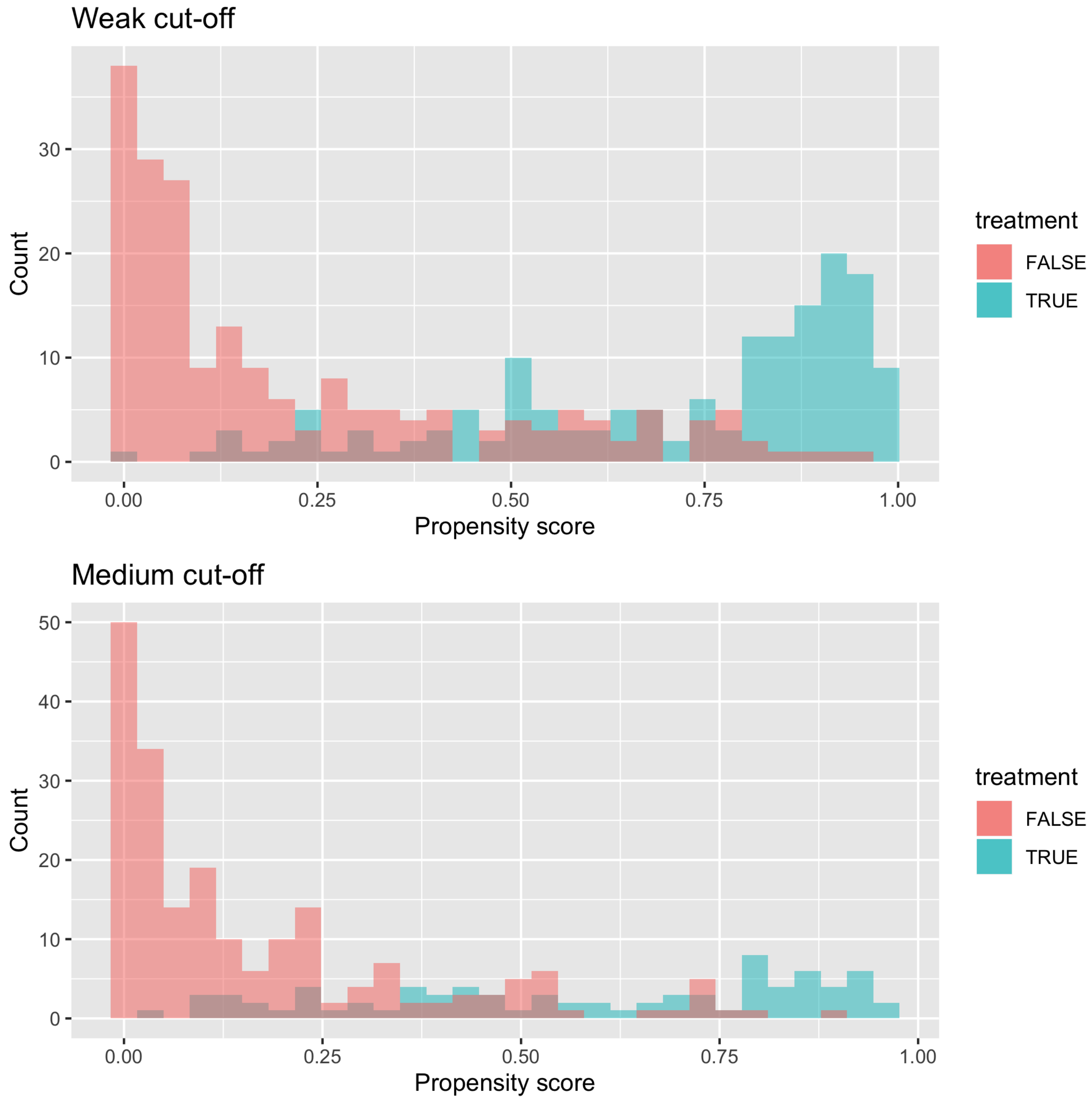
Figure 3 shows the distribution of the propensity scores for both treatment and control groups, and for weak and medium cut-off groups (note that matching was not performed for the strong cut-off group since there were insufficient matched observations for the ZINB regressions to converge). The propensity scores are in the range zero to one, with scores closer to one indicating that an observation is more likely to be a member of car-sharing given the observation’s characteristics. Control or treatment observations that fell out-with the distribution of the propensity scores of the other group were unmatched: 23 and 10 treatment observations from the weak and medium cut-off groups respectively. A second model including all observations was estimated so that the ATT could be estimated for the unmatched observations (see Section 3.5.1). Note, however, that the unmatched model is based on an extrapolation of the regression coefficients, and thus may be sensitive to model misspecification [29]. For the weak and medium cut-off groups, only the ZINB regression results of the matched models are shown; the unmatched regression results are available on request.

3.4. Zero-Inflated Negative Binomial Regressions

The results of the ZINB regressions for the weak, medium, and strong cut-off samples are presented in

Table 12. Logit regression results (weak cut-off, matched). Binary dependent variable: 0 km travelled by car.

Variable	Coefficient	Std. Error	z Value	Pr(>|z|)
treatment	1.017	0.518	1.963	0.050
csprovider	2.410	1.334	1.806	0.071
gender: male	−1.030	0.567	−1.818	0.069
log(pop.density)	0.624	0.377	1.654	0.098
companycar	2.738	0.932	2.936	0.003
hhpcars.pre.cs	−1.671	0.817	−2.046	0.041

,

Table 13. NB regression results (weak cut-off, matched). Dependent variable: total km travelled by car. (Note: * represents an interaction between variables.)

Variable	Coefficient	Std. Error	z Value	Pr(>|z|)
(Intercept)	7.069	1.393	5.074	0.000
treatment	−2.636	0.981	−2.687	0.007
cs.ff	0.544	0.964	0.565	0.572
csprovider	0.075	0.357	0.210	0.834
gender: male	0.393	0.127	3.105	0.002
environment: suburban	−0.365	0.205	−1.783	0.075
Region: Limburg	−1.092	0.458	−2.384	0.017
log(pop.density)	−0.256	0.144	−1.772	0.076
Q36_1N	−0.369	0.138	−2.674	0.007
treatment * hhpcars.pre.cs	2.428	1.268	1.914	0.056
treatment * hhpcars.pre.cs${}^2$	−0.678	0.360	−1.882	0.060
cs.ff * hhpcars.pre.cs	−0.713	0.669	−1.065	0.287

,

Table 14. Logit regression results (medium cut-off, matched). Binary dependent variable: 0 km travelled by car.

Variable	Coefficient	Std. Error	z Value	Pr(>|z|)
treatment	0.661	0.899	0.735	0.462
csprovider	3.291	2.709	1.215	0.224
gender: male	−3.376	1.765	−1.913	0.056
companycar	5.269	2.672	1.972	0.049
Q36_1N	−1.778	0.995	−1.788	0.074

,

Table 15. NB regression results (medium cut-off, matched). Dependent variable: total km travelled by car. (Note: * represents an interaction between variables.)

Variable	Coefficient	Std. Error	z Value	Pr(>|z|)
(Intercept)	5.505	1.513	3.638	0.000
treatment	−1.120	0.513	−2.184	0.029
hhpcars.pre.cs	0.766	0.280	2.734	0.006
cs.ff	−0.037	1.040	−0.036	0.972
csprovider	−0.556	0.488	−1.139	0.255
gender: male	0.446	0.167	2.676	0.007
environment: suburban	−0.696	0.271	−2.565	0.010
Region: Brussels	−1.882	0.584	−3.223	0.001
employment: other	1.298	0.732	1.774	0.076
treatment * hhpcars.pre.cs	0.463	0.364	1.272	0.203
cs.ff * hhpcars.pre.cs	−0.120	0.752	−0.160	0.873

,

Table 16. Logit regression results (strong cut-off, unmatched). Binary dependent variable: 0 km travelled by car.

Variable	Coefficient	Std. Error	z Value	Pr(>|z|)
(Intercept)	13.772	7.024	1.961	0.050
treatment	1.357	1.559	0.870	0.384
gender: male	−2.251	1.125	−2.001	0.045
hhadults	−1.687	0.700	−2.410	0.016
hhchildren	−1.477	0.749	−1.973	0.049
companycar	4.553	1.503	3.029	0.002
Q36_1N	−1.917	0.770	−2.490	0.013

and

Table 17. NB regression results (strong cut-off, unmatched). Dependent variable: total km travelled by car. (Note: * represents an interaction between variables.)

Variable	Coefficient	Std. Error	z Value	Pr(>|z|)
(Intercept)	6.619	1.137	5.820	0.000
treatment	0.225	0.642	0.351	0.725
hhpcars.pre.cs	0.812	0.134	6.079	0.000
csprovider	−0.364	0.749	−0.486	0.627
gender: male	0.539	0.133	4.068	0.000
hhadults	−0.165	0.093	−1.770	0.077
log(pop.density)	−0.259	0.148	−1.746	0.081
Region: Limburg	−0.607	0.277	−2.187	0.029
wrkscl.distance.wk	0.001	0.001	2.358	0.018
Q36_1N	−0.192	0.112	−1.705	0.088
treatment * hhpcars.pre.cs	−0.433	0.487	−0.888	0.374

. Regression coefficients for control variables with a p-value greater than 0.10 have been excluded for readability. It is not possible to directly interpret the coefficients in terms of their effect on the distance travelled by car, since the overall effect is a combination of both parts of the ZINB regressions (these results are presented in the next section). However, the signs of the regression coefficients are still meaningful, representing the influence the variable has on the direction of the dependent variables. In the medium and strong cut-off groups, one observation from the treatment group was excluded due to being an outlier, together with 13 observations from the control group. The treatment observation in question is the only respondent to have two cars in the household; the 13 controls are those who have three cars in the household (i.e., the counterfactual number of cars for the outlying treatment observation). Closer inspection of the outlier showed that the respondent is also the only car-sharing user who has a motorbike, and there are no corresponding controls with an equivalent number of cars and a motorbike. The reduced sample regressions are reported here, and should be more robust since they exclude this outlier.

The positive coefficient for the treatment variable in Table 12 shows that car-sharing users are more likely to not drive, all else being equal. Other significant results are that females, those with a company car, and those who do not believe there is too much traffic in Belgium are more likely to not drive at all.

The results of the NB regressions for the weak cut-off (Table 13) show that the impact of car-sharing on km driven by car does vary with the number of cars in the households, since the interactions with the number of household cars and the square of household cars are both significant. The results also show free-floating car-sharing users are expected to drive more than users of round-trip car-sharing, but that those who provide their own car are not significantly affected. The distance travelled by car is higher for males, while those who live in Limburg (relative to East Flanders), in areas of high population density, and those who believe there is too much traffic in Belgium are expected to reduce their distance travelled by car.

The logit regression results for the medium cut-off sample are similar to those of the weak cut-off group. For the NB regression, there is the perhaps unintuitive results that respondents who are more worried about particulates are likely to drive more. This may be reflective of a value-action gap amongst these respondents.

The logit regression results for the strong cut-off group show some differences relative to the other groups: having more adults and children in the household is associated with a lower likelihood of driving 0 km by car. In the NB regression results, although the coefficient for treatment is positive, when combined with the interaction with hhpcars.pre.cs (i.e., the counterfactual number of cars for car-sharing users, with minimum value of one), the overall treatment effect is still negative, that is, car-sharing is expected to reduce km driven by car, on average.

3.5. Average Treatment Effect on the Treated

3.5.1. Lower Access Users (LAUs)

The coefficients of the ZINB models are estimates, and thus contain some uncertainty. To estimate the ATT for LAUs with this uncertainty, we performed 1000 Monte Carlo simulations to estimate the regression coefficients from each of the models in Section 3.4. We assumed that the regression coefficients are part of a multivariate normal distribution, using estimated mean values and covariances from the results of the regression model. The ATT for each observation was then calculated for each of the simulations. For the unmatched observations in the weak and medium cut-off groups, the same procedure was applied using the results of regressions based on the whole sample (i.e., before matching). The estimated ATT for LAUs is thus a combination of the simulated results from both the matched and unmatched models.

The results of the simulated ATTs are presented in

Table 18. The estimated average treatment effect on the treated (ATT) for LAUs (change in km driven by car per user per week).

Cut-Off	Mean	Std Deviation	2.5% CI	97.5% CI
Weak	−93.8	16.5	−130.6	−64.1
Medium	−61.5	18.3	−101.1	−29.7
Strong	−54.3	30.2	−109.6	11.3

. The ATT for the for LAUs is progressively smaller (in absolute terms) as the cut-off becomes more strict. For LAUs, the ATT falls from an average decrease of 93.8 km in the weak cut-off group, to 61.5 km and 54.3 km for the medium and strong cut-off groups, respectively. The variation of the ATT (measured by the standard deviation) increases as the cut-off becomes more strict, owing to the progressively smaller number of LAUs.

3.5.2. Higher Access Users (HAUs)

For HAUs, there is no equivalent method to estimate the uncertainty of the ATT due to the method used to calculate the ATT. For HAUs with no cars in the household, the ATT is simply the distance travelled by shared car. For those who retain a car, the estimated ATT is based on a self-assessed counterfactual, which will be uncertain, but this uncertainty is not observed. Thus, the ATT for HAUs is a point estimate. The estimated ATT for HAUs are presented in

Table 19. The estimated ATT for HAUs (change in km driven by car per user per week).

Cutoff	Mean
Weak	31.5
Medium	33.1
Strong	35.6

.

3.5.3. Combined ATT

The overall ATT for each sample of car-sharing users is estimated by combining the results of LAUs and HAUs. The results for each cut-off group are given in

Table 20. The estimated ATT for the whole sample (change in km driven by car per user per week).

Cut-Off	Mean	Std Deviation	2.5% CI	97.5% CI
Weak	−54.07	11.19	−79.13	−33.90
Medium	−4.45	7.28	−20.17	8.16
Strong	24.19	3.82	17.21	32.49

. The confidence intervals represent the 2.5% and 97.5% percentiles of the combined ATT. Note that this uncertainty results from the Monte Carlo simulation of the LAUs only.

The overall ATT for car-sharing is very sensitive to the car-ownership effect. The ATTs for the weak cut-off sample is greater than zero in all simulations. However, for the medium cut-off sample the effect of car-sharing is not significantly different from zero. Finally, for the strong cut-off sample, the average effect is an increase in km driven by car for all simulations. The total change in car-use for each sample follows a similar pattern (

Table 21. The total change in km travelled by car caused by car-sharing.

Cut-Off	Mean	Std Deviation	2.5% CI	97.5% CI
Weak	−12,329	2550	−18,041	−7729
Medium	−886	1448	−4014	1624
Strong	4404	695	3132	5913

). Car-sharing leads to an overall reduction in car-use in 100% of simulations assuming weak cut-off, with a mean reduction of 12,329 km, but an overall increase in 100% of simulations assuming strong cut-off (mean increase 4,404 km). For the medium cut-off sample, car-sharing causes a reduction in car-use in 72.6% of simulations, with a mean reduction of 886 km per week.

3.6. Sensitivity Analysis: Oversampling of p2p Car-Sharing

To assess the effect of the oversampling of p2p car-sharing users, matched models including p2p membership (interacted with number of household cars) were estimated for both the weak and medium cut-off groups. The regression coefficients and their significance suggest that the inclusion of p2p users does not lead to a significantly better fit (see

Table A1. Logit regression coefficients for treatment and p2p variables (weak cut-off). Dependent variable: 0 km travelled by car.

Variable	Coefficient	Std. Error	z Value	Pr(>|z|)
treatment	1.092	0.572	1.909	0.056
p2p	−0.169	0.553	−0.307	0.759

,

Table A2. NB regression coefficients for treatment and p2p variables (weak cut-off). Dependent variable: km travelled by car. (Note: * represents an interaction between variables.)

Variable	Coefficient	Std. Error	z Value	Pr(>|z|)
treatment	−2.761	1.165	−2.370	0.018
p2p	0.433	1.570	0.276	0.783
treatment * hhpcars.pre.cs	2.428	1.525	1.592	0.111
treatment * hhpcars.pre.cs${}^2$	−0.643	0.444	−1.447	0.148
p2p * hhpcars.pre.cs	−0.236	2.062	−0.115	0.909
p2p * hhpcars.pre.cs${}^2$	−0.033	0.589	−0.055	0.956

,

Table A3. Logit regression coefficients for treatment and p2p variables (medium cut-off). Dependent variable: 0 km travelled by car.

Variable	Coefficient	Std. Error	z Value	Pr(>|z|)
treatment	0.390	1.031	0.378	0.705
p2p	0.616	1.038	0.594	0.553

and

Table A4. NB regression coefficients for treatment and p2p variables (medium cut-off). Dependent variable: km travelled by car. (Note: * represents an interaction between variables.)

Variable	Coefficient	Std. Error	z Value	Pr(>|z|)
treatment	−1.157	0.604	−1.916	0.055
p2p	0.056	0.755	0.074	0.941
treatment * hhpcars.pre.cs	0.474	0.416	1.137	0.255
p2p * hhpcars.pre.cs	0.009	0.530	0.016	0.987

in the Appendix A). To confirm this, we performed likelihood ratio tests for both weak and medium cut-off groups, with the null hypothesis that the fit of the models presented in Section 3.4 are the same as the models with p2p variables included. The results of the likelihood ratio tests confirm that the model without the inclusion of p2p users is preferred: we fail to reject the null hypothesis in both the weak and medium cut-off groups (

Table 22. Likelihood ratio test (weak cut-ff). Null hypothesis: no difference between models.

Model	LogLik	$\Delta$ Deg. freedom	Chisq	Pr(>Chisq)
Base	−1388.91
p2p effects	−1388.37	4	1.08	0.898

and

Table 23. Likelihood ratio test (medium cut-off). Null hypothesis: no difference between models.

Model	LogLik	$\Delta$ Deg. freedom	Chisq	Pr(>Chisq)
Base	−688.46
p2p effects	−688.25	3	0.42	0.936

). In other words, the oversampling of p2p users does not have a significant effect on the overall estimate.

4. Discussion

4.1. The Effect of Car-Sharing on Car-Ownership and Car-Use

The results show that the impact of car-sharing on car-use is very variable, ranging from a statistically significant reduction of car-use by 56 km per user per day, to an increase of 24 km (also statistically significant). This variability derives from the high sensitivity to the car-ownership effect. The estimated car-ownership effect depends on how confident one can be in the self-assessed counterfactual. The results in Table 11 show that, given the weak, medium, and strong cut-offs, 69.3%, 40% and 12.6% of users, respectively, have one fewer car because of car-sharing. In comparison to the results in studies in Section 1.1, the weak cut-off group would be appear to be an outlier: no other study estimates such a large effect. Moreover, the two studies that use quasi-experimental methods for round-trip car-sharing estimate a much smaller reduction in car ownership than both the weak and medium cut-off groups [9,13], although this difference could be due to different time and geographical contexts. The results given the medium cut-off group are similar to other studies of round-trip car-sharing in Europe that make use of self-assessed counterfactuals ([7,14,15,16]).

The estimated car-use ATT for LAUs is progressively smaller as the cut-off is made more strict, implying that users who are more certain of the effect of car-sharing on car-ownership reduce their car-use by less. This effect, together with the change in the relative number of HAUs and LAUs, mean that the overall treatment effect of car-sharing on car-use varies, in both size and sign. Only in the weak cut-off group is the estimated overall treatment effect significantly less than zero, with an average reduction in car-use of 54.1 km per user per week. In the medium cut-off group, the estimated ATT is much smaller: an average reduction of 4.4 km per user per week; in fact, in 28% of simulations, car-sharing led to an increase in car-use in the medium cut-off group. Finally, the estimated ATT based on the strong cut-off group implies that car-sharing users increase their car-use by 24.2 km per user per week, on average. Comparing the results to studies reviewed in Section 1.1, our results generally imply a smaller reduction in car-use. For example, in other European-based studies, Nijland and van Meerkerk [14] estimated car-sharing users in the Netherlands reduce km driven by car by 33.7 km per user per week, on average, while car-sharing users in London reduce their km travelled by car by 17.3 km per user per week, on average [15]. Thus, both the car-ownership effect and the ATT estimated for the weak cut-off group appear to be outliers compared to the other European studies. These results would seem to add weight to other recent studies that have found that car-sharing may not be as environmentally beneficial as previously thought [5,6,28].

4.2. Policy Implications

Policy intervention may be required to ensure that car-sharing leads to a substantial reduction in car-use, and all the associated environmental benefits that that would bring. The sensitivity of car-use impacts to changes in car-ownership suggests that policies designed to reduce car-ownership would help to realise larger reductions in car-use. However, making car-sharing cheaper may result in substitution effects that reduce public transport use instead of car-use. Thus, policy strategies that focus on making car-ownership less attractive are likely to lead to lower car-use, and thus lower emissions, in the long-run. For example, an effective policy mix designed to increase the number of LAUs relative to HAUs could be to make car-ownership more expensive through higher one-off taxes at sale (in contrast to some discussions on the topic of car taxes, where the focus has been on shifting taxes to car-use rather than car-ownership: see van Dender [38] for example). Policy makers could also make car-ownership less convenient by limiting the number of parking spaces or increasing parking costs. Additionally, limiting the fiscal benefits of company cars may lead to less effective car-ownership, a particular issue in Belgium [39]. However, these policies involve different levels of government (federal, regional and city/municipal) and different actors (car-sharing firms, company car fleet operators, businesses, employees, consumers) that make a coordinated policy mix a complex multi-level governance problem, especially in Belgium [40]. In Belgium, the fiscal treatment of cars and company cars is a federal responsibility. These policies would thus affect the national population, despite car-sharing being mainly an urban phenomenon. However, low emission zones (LEZs) present an opportunity for city governments to affect car-ownership. LEZs have been introduced in many Flemish cities aimed at reducing air pollution caused by particulates; to ease the transition, residents are offered incentives to scrap cars that no longer meet LEZ requirements. By manipulating the incentives offered, car-ownership may be reduced at the expense of a more multi-modal lifestyle that includes occasional car-use through car-sharing. For example, in-kind incentives such as public transport passes, bike sharing memberships or car-sharing memberships may lead to residents choosing to forgo the replacement of their cars. Cash incentives, however, risk residents offsetting the cost of a new car purchase instead.

An interesting finding from the survey is that there appears to be a value-action gap amongst some car-sharing users. For example, almost all HAUs think that there is too much traffic in Belgium and are worried about climate change. This suggests that such users are not aware that their actions, that is, (excessive) car-use, are still causing environmental harm. Thus, there is a need to continue to promote alternative modes of transport (including both public transport and active modes) at the expense of all car-use, both shared and private. This may allow HAUs to act more in accordance with their values.

The differences in characteristics between HAUs and LAUs are not clear from this survey. Further research is therefore needed to better understand why some users see car-sharing as a replacement for car-ownership. This could help policymakers better understand how to specifically target such users.

4.3. Implications for Research: Limitations and Recommendations

There is a need to move beyond self-assessed counterfactuals in the evidence base and move towards quasi-experimental methods, as is standard in impact evaluation. We have made first step towards this, but there remain some limitations that should be addressed.

The effect of car-sharing on car-ownership is made up of two effects: users who get rid of a car because they joined car-sharing, and users who would have purchased a car if they had not joined car-sharing. The first of these effects relies on users being able to attribute the effect to car-sharing, and not to another event. Systematic errors in this estimate are known as attribution bias. The second effect relies on users being able to estimate a hypothetical future. Research has shown that when program participants (e.g., car-sharing users) are asked hypothetical questions, a number of biases will cause them to make inaccurate predictions about their behaviour [23]. It is therefore crucial that there is continued research on the effects of car-sharing on car-ownership using quasi-experimental methods, where possible, and thus avoiding the biases inherent in a self-assessed approach. As discussed in Section 2.3, due to the problems posed by reverse causality, quasi-experiential methods using longitudinal data present the most robust method of estimating the car-ownership effect (e.g., Becker et al. [8]), although Mishra et al. [13] present a quasi-experimental approach that uses cross-sectional data.

The quasi-experimental procedure for estimating the impact on car-use for LAUs (i.e., sample pre-screening, matching, ZINB regressions) could be replicated in future car-sharing studies. Ideally, the same procedure would be used to estimate the impact on car-use for the minority of HAUs who retain a car, which was not possible in this study; instead, this impact was estimated using a self-assessed counterfactual and thus there could remain some self-assessment bias for these users.

The major threat to external validity in this study is the sample. As discussed in Section 2.1, the research design aimed to reach as many car-sharing users as possible; however, as a result, it is not necessarily representative of the car-sharing population in Flanders. While steps have been taken to control for this issue (e.g., Section 3.6), it cannot be ruled out that some sampling bias remains. A representative sample of car-sharing users, across different systems, locations, demographics, and so forth, would allow for more confidence in the external validity of results. Such samples may be easier to collect as car-sharing becomes more popular, or if researchers are able to gather data with the consent of car-sharing firms.

5. Conclusions

Car-sharing may be a promising system that can deliver a reduction in car-use, and consequently help to lower GHG emissions, air pollution, and traffic congestion. Existing studies have tended to show that car-sharing does lead to lower car-use; however there have been very few studies making use of quasi-experimental methods, and instead most impact studies rely exclusively on users’ own assessment of their change in behaviour. In this study, we have used a quasi-experimental method to estimate the change in car-use. The results show that the key driver in car-sharing being able to reduce car-use is its effect on car-ownership: users who reduce car-ownership will reduce their car-use (LAUs), while those for whom car-sharing has no effect on car-ownership will increase their car-use (HAUs). According to our results, only by assuming that car-sharing has a large effect on car-ownership (i.e., the weak cut-off group) will car-sharing lead to a statistically significant reduction in car-use. This suggests that policy intervention may be required to ensure the full environmental benefits of car-sharing are realised. Policies should focus on encouraging car-sharing at the expense of car-ownership, for example, by increasing the tax burden associated with car-ownership, or by reducing the convenience of car-ownership through stricter parking regulations. However, policies that make car-sharing more attractive (e.g., through tax breaks or preferential parking/traffic policies) risk attracting HAUs as much as LAUs, and consequently risk stimulating more car-use. Such policies should therefore be subject to rigorous ex-ante and ex-post evaluations to ensure reductions in car-use actually occur.

The estimated impact of car-sharing on car-use and the sensitivity of this to car-ownership effects highlighted in this study show the need for more robust, quasi-experimental research into the impacts of car-sharing on both car-ownership and car-use. Future studies could build on this research by using either longitudinal data or an instrumental variable approach that would allow both of these impacts to be estimated without the need for self-assessment. However, collection of this data remains a challenge, especially while car-sharing is a niche activity.

References

- IPCC. Summary for Policymakers. In Climate Change 2014, Mitigation of Climate Change. Contribution of Working Group III to the Fifth Assessment Report of the Intergovernmental Panel on Climate Change; Edenhofer, O., Pichs-Madruga, R., Sokona, Y., Farahani, E., Kadner, S., Seyboth, K., Adler, A., Baum, I., Brunner, S., Eickemeier, P., et al., Eds.; Cambridge University Press: Cambridge, UK; New York, NY, USA, 2014. [Google Scholar]
- Material Economics. The Circular Economy, a Powerful Force for Climate Mitigation. Available online: https://materialeconomics.com/publications/the-circular-economy (accessed on 28 September 2020).
- Martin, E.; Shaheen, S.A. Greenhouse Gas Emissions Impacts of Carsharing in North America. Trans. Intell. Transp. Syst. 2011, 12, 1074–1086. [Google Scholar] [CrossRef] [Green Version]
- Chen, T.D.; Kockelman, K.M. Carsharing’s Life-Cycle Impacts on Energy Use and Greenhouse Gas Emissions. Transp. Res. Part D Transp. Environ. 2016, 47, 276–284. [Google Scholar] [CrossRef]
- Amatuni, L.; Ottelin, J.; Steubing, B.; Mogollón, J.M. Does Car Sharing Reduce Greenhouse Gas Emissions? Assessing the Modal Shift and Lifetime Shift Rebound Effects from a Life Cycle Perspective. J. Clean. Prod. 2020, 266, 121869. [Google Scholar] [CrossRef]
- Jung, J.; Koo, Y. Analyzing the Effects of Car Sharing Services on the Reduction of Greenhouse Gas (GHG) Emissions. Sustainability 2018, 10, 539. [Google Scholar] [CrossRef] [Green Version]
- 6T-Bureau De Recherche. One-Way Carsharing: Which Alternative to Private Car? The Case Study of Autolib’ in Paris; 6T-Bureau De Recherche: Paris, France, 2014. [Google Scholar]
- Becker, H.; Ciari, F.; Axhausen, K.W. Measuring the Car Ownership Impact of Free-Floating Car-Sharing— A Case Study in Basel, Switzerland. Transp. Res. Part D Transp. Environ. 2018, 65, 51–62. [Google Scholar] [CrossRef] [Green Version]
- Cervero, R.; Golub, A.; Nee, B. City CarShare: Longer-Term Travel Demand and Car Ownership Impacts. Transp. Res. Rec. J. Transp. Res. Board 2007, 70–80. [Google Scholar] [CrossRef]
- Firnkorn, J.; Müller, M. Selling Mobility Instead of Cars: New Business Strategies of Automakers and the Impact on Private Vehicle Holding. Bus. Strategy Environ. 2012, 21, 264–280. [Google Scholar] [CrossRef]
- Giesel, F.; Nobis, C. The Impact of Carsharing on Car Ownership in German Cities. Transp. Res. Procedia 2016, 19, 215–224. [Google Scholar] [CrossRef] [Green Version]
- Martin, E.; Shaheen, S.; Lidicker, J. Impact of Carsharing on Household Vehicle Holdings. Transp. Res. Rec. J. Transp. Res. Board 2010, 2143, 150–158. [Google Scholar] [CrossRef]
- Mishra, G.S.; Mokhtarian, P.L.; Clewlow, R.R.; Widaman, K.F. Addressing the Joint Occurrence of Self-Selection and Simultaneity Biases in the Estimation of Program Effects Based on Cross-Sectional Observational Surveys: Case Study of Travel Behavior Effects in Carsharing. Transportation 2019, 46, 95–123. [Google Scholar] [CrossRef]
- Nijland, H.; van Meerkerk, J. Mobility and Environmental Impacts of Car Sharing in the Netherlands. Environ. Innov. Soc. Transit. 2017, 23, 84–91. [Google Scholar] [CrossRef]
- Wu, C.; Le Vine, S.; Clark, M.; Gifford, K.; Polak, J. Factors Associated with Round-Trip Carsharing Frequency and Driving-Mileage Impacts in London. Int. J. Sustain. Transp. 2020, 14, 177–186. [Google Scholar] [CrossRef]
- Le Vine, S.; Polak, J. The Impact of Free-Floating Carsharing on Car Ownership: Early-Stage Findings from London. Transp. Policy 2019, 75, 119–127. [Google Scholar] [CrossRef]
- Kim, D.; Park, Y.; Ko, J. Factors Underlying Vehicle Ownership Reduction among Carsharing Users: A Repeated Cross-Sectional Analysis. Transp. Res. Part Transp. Environ. 2019, 76, 123–137. [Google Scholar] [CrossRef]
- Becker, H.; Ciari, F.; Axhausen, K.W. Comparing Car-Sharing Schemes in Switzerland: User Groups and Usage Patterns. Transp. Res. Part A Policy Pract. 2017, 97, 17–29. [Google Scholar] [CrossRef] [Green Version]
- Martin, E.; Shaheen, S. Impacts of Car2go on Vehicle Ownership, Modal Shift, Vehicle Miles Travelled, and Greenhouse Gas Emissions: An Analysis of Five North American Cities. Available online: https://tsrc.berkeley.edu/publications/impacts-car2go-vehicle-ownership-modal-shift-vehicle-miles-traveled-and-greenhouse-gas (accessed on 28 September 2020).
- Gertler, P.J.; Martinez, S.; Premand, P.; Rawlings, L.B.; Vermeersch, C.M.J. Impact Evaluation in Practice, 2nd ed.; Inter-American Development Bank and World Bank: Washington, DC, USA, 2016; ISBN 978-1-4648-0780-0. [Google Scholar]
- Ravallion, M. The Mystery of the Vanishing Benefits: An Introduction to Impact Evaluation. World Bank Econ. Rev. 2001, 15, 115–140. [Google Scholar] [CrossRef]
- Hill, L.G.; Betz, D.L. Revisiting the Retrospective Pretest. Am. J. Eval. 2005, 26, 501–517. [Google Scholar] [CrossRef]
- Mueller, C.E.; Gaus, H. Assessing the Performance of the “Counterfactual as Self-Estimated by Program Participants”: Results From a Randomized Controlled Trial. Am. J. Eval. 2015, 36, 7–24. [Google Scholar] [CrossRef]
- StatBel. Structure of the Population. Available online: https://statbel.fgov.be/en/themes/population/structure-population (accessed on 28 September 2020).
- Beeckman, H. Autodelen Wint Snel Aan Populariteit, Maar Lost Dat Onze Files Op? VRT, [Online]. 14 September 2019. Available online: https://www.vrt.be/vrtnws/nl/2019/09/14/autodelen-wint-snel-aan-populariteit-maar-lost-dat-onze-files-o/(accessed on 28 September 2020).
- freeworldmaps.net. Flanders Maps. Available online: https://www.freeworldmaps.net/europe/belgium/flanders.html (accessed on 28 September 2020).
- Imbens, G.W.; Rubin, D.B. Causal Inference for Statistics, Social, and Biomedical Sciences: An Introduction; Cambridge University Press: Cambridge, UK, 2015; ISBN 978-113-902-575-1. [Google Scholar]
- Ke, H.; Chai, S.; Cheng, R. Does Car Sharing Help Reduce the Total Number of Vehicles? Soft Comput. 2019, 23, 12461–12474. [Google Scholar] [CrossRef]
- Gelman, A.; Hill, J. Data Analysis Using Regression and Multilevel/Hierarchical Models; Analytical Methods for Social Research; Cambridge University Press: Cambridge, UK, 2006; Chapter 10; pp. 199–234. [Google Scholar]
- Ho, D.E.; Imai, K.; King, G.; Stuart, E.A. MatchIt: Nonparametric Preprocessing for Parametric Causal Inference. J. Stat. Softw. 2011, 42, 1–28. [Google Scholar] [CrossRef] [Green Version]
- R Core Team. R: A Language and Environment for Statistical Computing; R Foundation for Statistical Computing: Vienna, Austria, 2019. [Google Scholar]
- Lambert, D. Zero-Inflated Poisson Regression, with an Application to Defects in Manufacturing. Technometrics 1992, 34, 1. [Google Scholar] [CrossRef]
- Zeileis, A.; Kleiber, C.; Jackman, S. Regression Models for Count Data in R. J. Stat. Softw. 2008, 27, 1–25. [Google Scholar] [CrossRef] [Green Version]
- Jackman, S. Pscl: Classes and Methods for R Developed in the Political Science Computational Laboratory; United States Studies Centre, University of Sydney: Sydney, Australia, 2020. [Google Scholar]
- Albert, J.M.; Wang, W.; Nelson, S. Estimating Overall Exposure Effects for Zero-Inflated Regression Models with Application to Dental Caries. Stat. Methods Med Res. 2014, 23, 257–278. [Google Scholar] [CrossRef] [PubMed] [Green Version]
- Gelman, A.; Hill, J. Data Analysis Using Regression and Multilevel/Hierarchical Models; Analytical Methods for Social Research; Cambridge University Press: Cambridge, UK, 2006; Chapter 9; pp. 167–198. [Google Scholar]
- Namazu, M.; Dowlatabadi, H. Vehicle Ownership Reduction: A Comparison of One-Way and Two-Way Carsharing Systems. Transp. Policy 2018, 64, 38–50. [Google Scholar] [CrossRef]
- Van Dender, K. Taxing Vehicles, Fuels, and Road Use: Opportunities for Improving Transport Tax Practice; OECD Taxation Working Papers 44; OECD: Paris, France, 2019. [Google Scholar] [CrossRef]
- May, X.; Ermans, T.; Hooftman, N. Company Cars: Identifying the Problems and Challenges of a Tax System. Brussels Studies. [Online], Synopses, no. 133. 25 March 2019. Available online: http://journals.openedition.org/brussels/2499 (accessed on 28 September 2020). [CrossRef]
- Happaerts, S. Climate Governance in Federal Belgium: Modest Subnational Policies in a Complex Multi-Level Setting. J. Integr. Environ. Sci. 2015, 12, 285–301. [Google Scholar] [CrossRef] [Green Version]
Figure 1.
Map of Flanders showing the regions and major cities [26].
Figure 2.
Causal diagram on the relation between, car-sharing, car-ownership and car-use. The dashed arrows are mutually exclusive. Green arrows represent a positive relationship (increase [decrease] in one causes an increase [decrease] in the other); red arrows represent a negative relationship (increase [decrease] in one causes a decrease [increase] in the other).
Figure 3.
Histograms showing the distribution of propensity scores for both weak and medium samples, by treatment and control groups.