Article

Extreme Learning Machine Based Prediction of Soil Shear Strength: A Sensitivity Analysis Using Monte Carlo Simulations and Feature Backward Elimination

1
Division of Computational Mathematics and Engineering, Institute for Computational Science, Ton Duc Thang University, Ho Chi Minh City 700000, Vietnam
2
Faculty of Civil Engineering, Ton Duc Thang University, Ho Chi Minh City 700000, Vietnam
3
University of Transport Technology, Hanoi 100000, Vietnam
4
University of Transport and Communications, Hanoi 100000, Vietnam
5
Department of Civil, Environmental and Natural Resources Engineering, Lulea University of Technology, 971 87 Lulea, Sweden
6
Institute of Research and Development, Duy Tan University, Da Nang 550000, Vietnam
*
Authors to whom correspondence should be addressed.
Sustainability 2020, 12(6), 2339; https://doi.org/10.3390/su12062339
Submission received: 9 February 2020 / Revised: 12 March 2020 / Accepted: 16 March 2020 / Published: 17 March 2020

Abstract

:
Machine Learning (ML) has been applied widely in solving a lot of real-world problems. However, this approach is very sensitive to the selection of input variables for modeling and simulation. In this study, the main objective is to analyze the sensitivity of an advanced ML method, namely the Extreme Learning Machine (ELM) algorithm under different feature selection scenarios for prediction of shear strength of soil. Feature backward elimination supported by Monte Carlo simulations was applied to evaluate the importance of factors used for the modeling. A database constructed from 538 samples collected from Long Phu 1 power plant project was used for analysis. Well-known statistical indicators, such as the correlation coefficient (R), root mean squared error (RMSE), and mean absolute error (MAE), were utilized to evaluate the performance of the ELM algorithm. In each elimination step, the majority vote based on six elimination indicators was selected to decide the variable to be excluded. A number of 30,000 simulations were conducted to find out the most relevant variables in predicting the shear strength of soil using ELM. The results show that the performance of ELM is good but very different under different combinations of input factors. The moisture content, liquid limit, and plastic limit were found as the most critical variables for the prediction of shear strength of soil using the ML model.

1. Introduction

In the design phase of various large-scale construction projects (highways, roads, high rise buildings) and geotechnical structures (earth dams, retaining walls), shear strength is an important factor used to define the capability of soil foundations [1]. The shear strength of soil is determined using Mohr–Coulomb criteria through two parameters, namely unit cohesion (c) and internal friction angle ( φ ) in the case of normal soil or only unit cohesion (c) in the case of sandy soil [1]. However, to determine these parameters, the consuming time and costly experiments are often carried out in the laboratory, including direct shear test, triaxial compression tests, or unconfined compression tests which might increase the cost and prolong the time of completing the projects. Moreover, the test accuracy depends significantly on the instruments, the meticulous procedures, and the expertise of the experimenters [1]. Therefore, the development of new advanced techniques for quick and accurate prediction of shear strength of soil is essential and practical.
Traditionally, the shear strength of soil is often predicted by using traditional formula-based methods. Garven and Vanapalli [2] summarized and evaluated nineteen empirical techniques that are available for the prediction of the shear strength of unsaturated soils. Out of these, six techniques used tool of the soil-water retention curve (SWRC) and the remainder thirteen procedures are based on mathematical formulations. In these empirical techniques, various parameters of soil were used to correlate with the shear strength in unsaturated soils such as the texture of soil surface, pore size distribution, residual suction. In another study, Sheng et al. [3] proposed different empirical equations for the prediction of shear strength of unsaturated soils using different approaches, which are based on the independent stress, Bishop’s stress, and constitutive models. Vanapalli and Fredlund [4] compared different empirical approaches for the prediction of shear strength of unsaturated soils. Various parameters used for forming the correlation equations such as particle gain distribution, liquid limit, plasticity indices, water content. Al Aqtash and Bandini [5] used the soil-water characteristic curve to predict the unsaturated shear strength of an adobe soil. In general, these studies show the suitability of these approaches for predictions of the shear strength of soil. However, these approaches might not produce predictive results with satisfactory accuracy as they are based on the linear assumption of the factors used and non-multivariate models [1].
More recently, advanced data-driven methods based on computational algorithms, like machine learning (ML) approaches, have been developed and applied for the construction of soil shear strength prediction models. They are known as excellent models with high predictive capability as they are useful in discovering the nonlinear relationship inside the data and are capable of considering many input variables in the prediction of shear strength of soil [1]. These models are also flexible as they can adjust their model structures to be suitable with the changes in the data. Tien Bui et al. [1] developed a swarm intelligence-based ML approach (LSSVM-CSO) to predict soil shear strength for road construction. A number of geotechnical factors were used in the model, such as sample depth, sand percentage, loam percentage, clay percentage, moisture content, wet density, of soil, specific gravity, liquid limit, plastic limit, plastic index, and liquid index. The results of this study showed that the proposed model has a good predictive capability in the prediction of soil shear strength. This model outperformed other benchmark ML models, namely least squares support vector machine (LSSVM), artificial neural network (ANN), and regression tree (RT). Pham et al. [6] developed two hybrid advanced ML techniques, namely GANFIS and PANFIS, for prediction of soil shear strength and compared these hybrid models with two other benchmark models, namely ANN and Support Vector Regression (SVR). The results showed that the proposed hybrid models outperformed benchmark models with outstanding predictive accuracy. Prediction of shear strength using ML approaches is also an interesting topic of many studies [7,8].
Although advanced ML approaches are good compared with traditional approaches, these models are very sensitive to the selection of input parameters used in the modeling. Das et al. [9] investigated the performance of two popular ML methods, namely SVM and ANN, for prediction of soil shear strength under the effects of different input properties and stated that the performance of SVM and ANN are good but very different under the effects of different input properties. The study also suggested to carry out the sensitivity analysis to select the best suitable factors for developing and applying the ML models. The same observation has been pointed out in other studies of Nguyen et al. [10] and Pham et al. [11]. However, these studies used a trial-manual process for sensitivity analysis, which might not cover all the cases of variation of input parameters. Therefore, in this study, the main objective is to use two advanced computational statistical methods such as Monte Carlo simulation and Feature Backward Elimination for evaluation of the sensitivity analysis of an advance ML technique, namely Extreme Learning Machine (ELM) algorithm for prediction of soil shear strength. The main contribution of this study to the knowledge body is that (i) it proposes a soft computing technique (ELM) for quick and accurate prediction of soil shear strength considering more input parameters, which is limited or not easy to be done by using the empirical correlation equation, (ii) it evaluates for the first time the performance of ELM under different combination of input parameters using Monte Carlo simulation and Feature Backward Elimination, which will help in suitable selection of parameters for prediction of soil shear strength using soft computing techniques. For this aim, data of 538 soil samples collected from the Long Phu 1 power plant project, Long Phu district, Soc Trang province, Vietnam were used for generating the datasets used in the modeling. Well-known statistical indicators, such as the correlation coefficient (R), root mean squared error (RMSE), and mean absolute error (MAE), were utilized to evaluate the performance of the ELM algorithm under sensitivity analysis.

2. Methodology

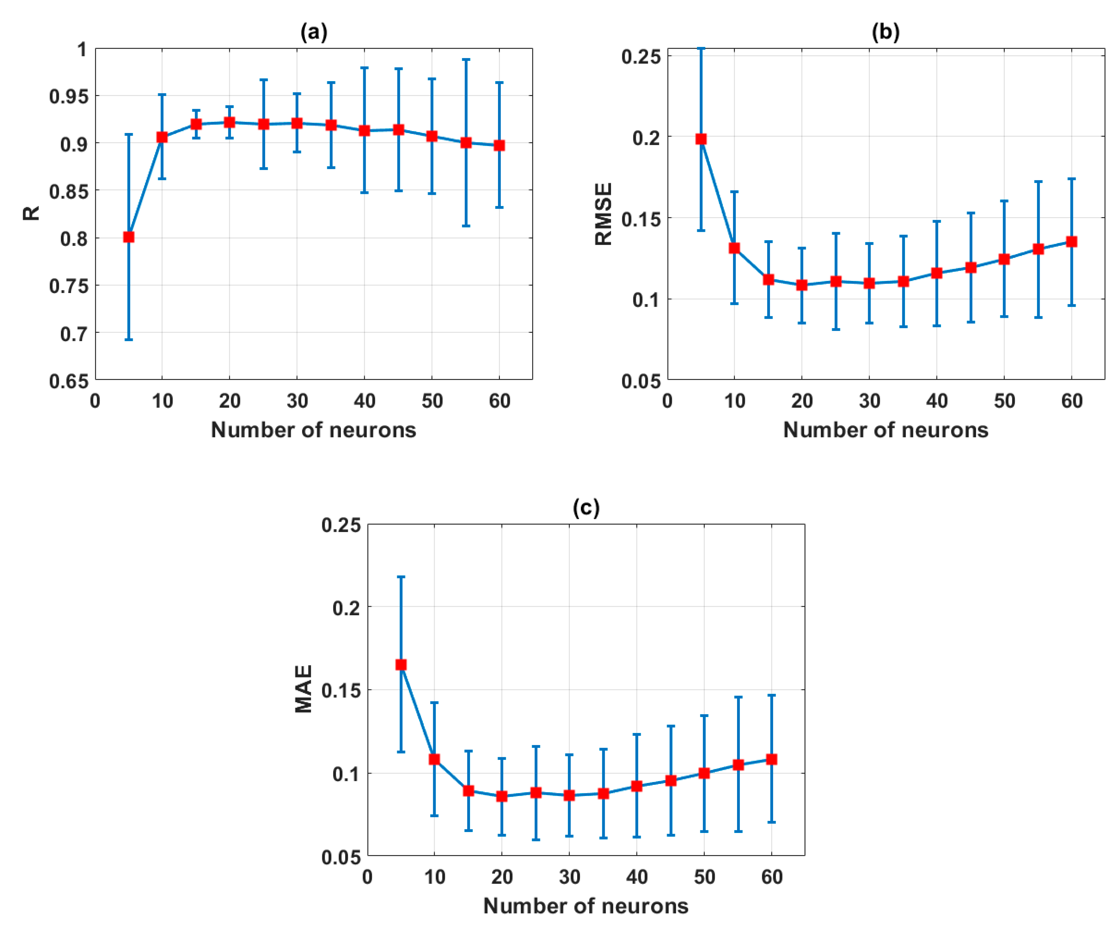
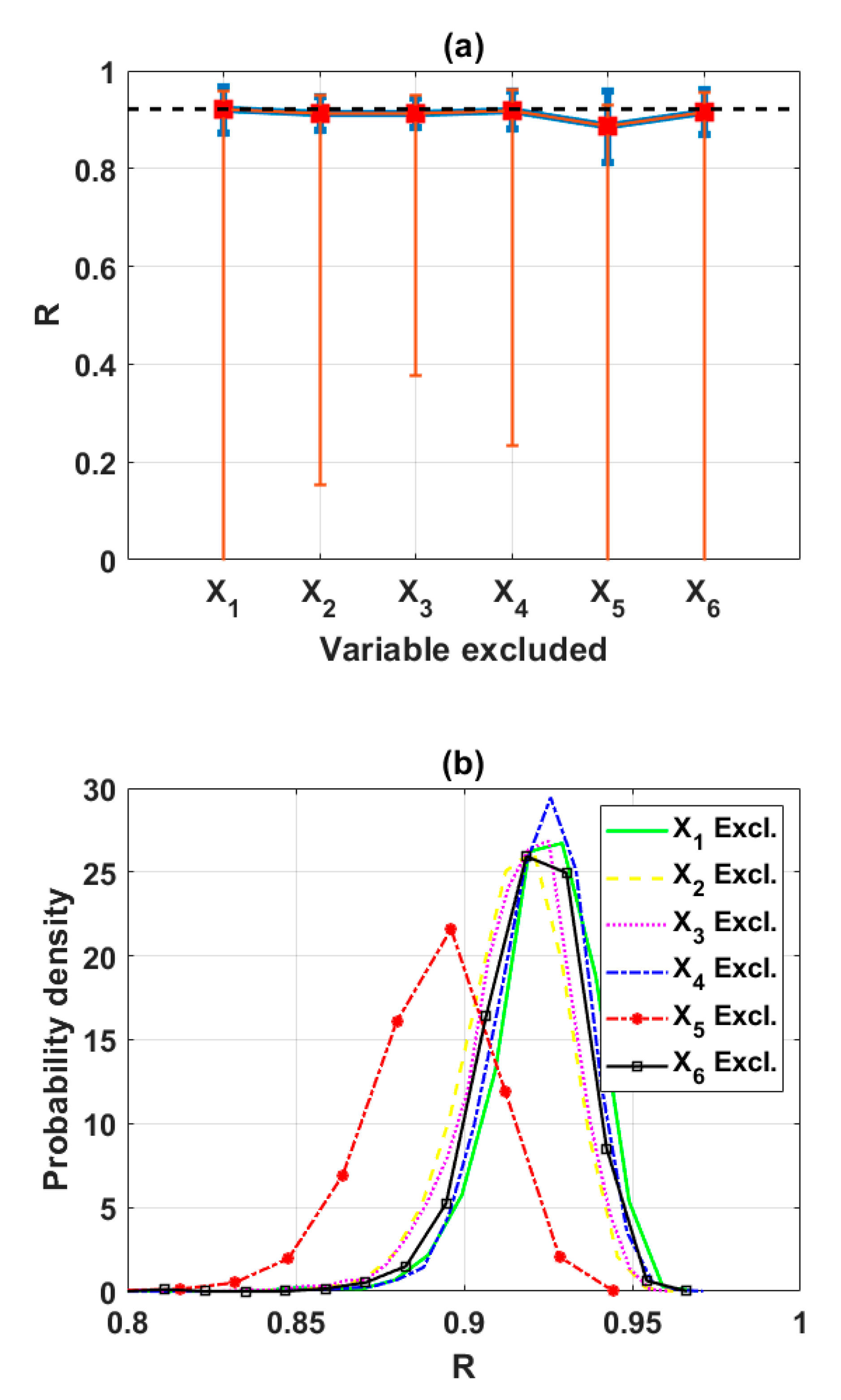
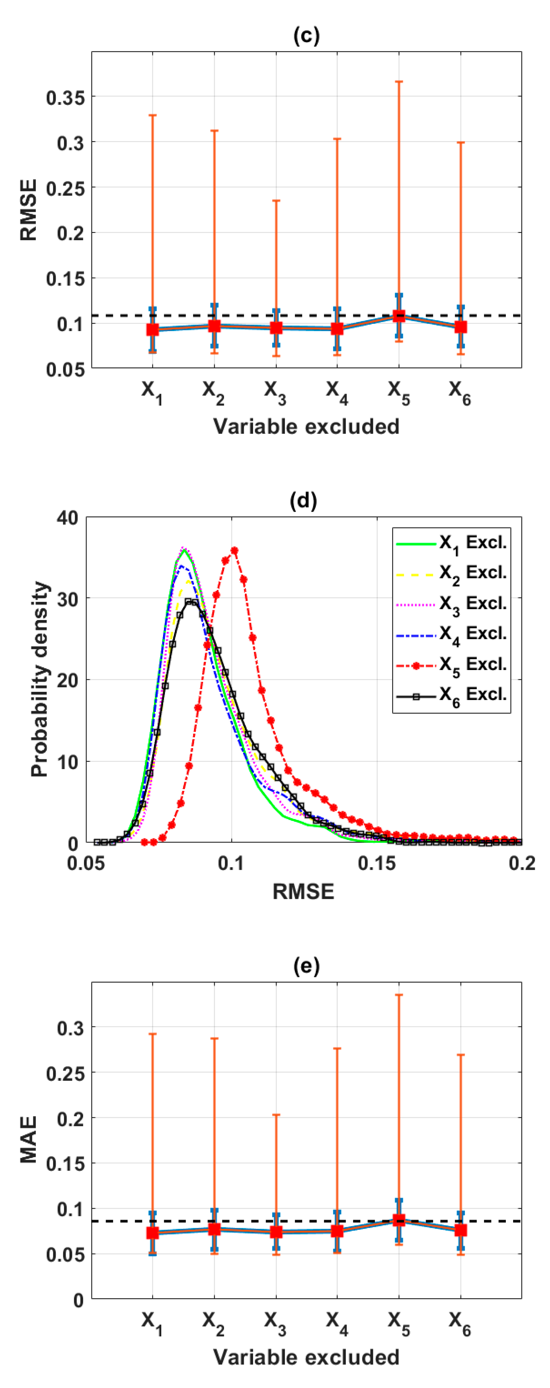
In order to address this problem, the methodology of the present study contains several main steps such as (1) construction of the database: Input parameters, namely the clay content, moisture content, specific gravity, void ratio, liquid limit, and plastic limit were gathered from technical reports. The considered output variable of this work is the shear strength of soil, (2) ELM algorithm was firstly optimized by an analysis concerning the number of neurons used in the model, (3) after the optimal number of neurons of ELM successfully found, it was used to perform the backward elimination in combination with Monte Carlo simulation, (4) using six types of criteria, namely the maximum value of R, minimum values of RMSE and MAE, average values of R, RMSE and MAE, the elimination of input variables was decided by majority vote.

2.1. Data Collection and Preparation

Data used in this study were collected from the Long Phu 1 power plant project (longitude of 9°59′07.3″N and latitude of 106°04′48″E) located at the southern side of the Hau river, Long Duc commune, Long Phu district, Soc Trang province, Vietnam (Figure 1). Union of Engineering Geology, Construction and Environment (UGCE) was in charge of the soil investigation works. In addition, a program of the additional soil investigation was carried out by UGCE in April and August 2011, including exploratory borings, field testing, and soil laboratory testing to provide the information relating to the soil conditions of foundation design and construction of the project, and these data were extracted to generate the datasets for the modeling of soil shear strength prediction in this study.
Datasets of 538 soil samples were extracted from the project and used in this study. In datasets, variables, such as moisture content (%), clay content (%), void ratio, plastic limit (%), liquid limit (%), and specific gravity, were used as inputs, and shear strength was used as output.
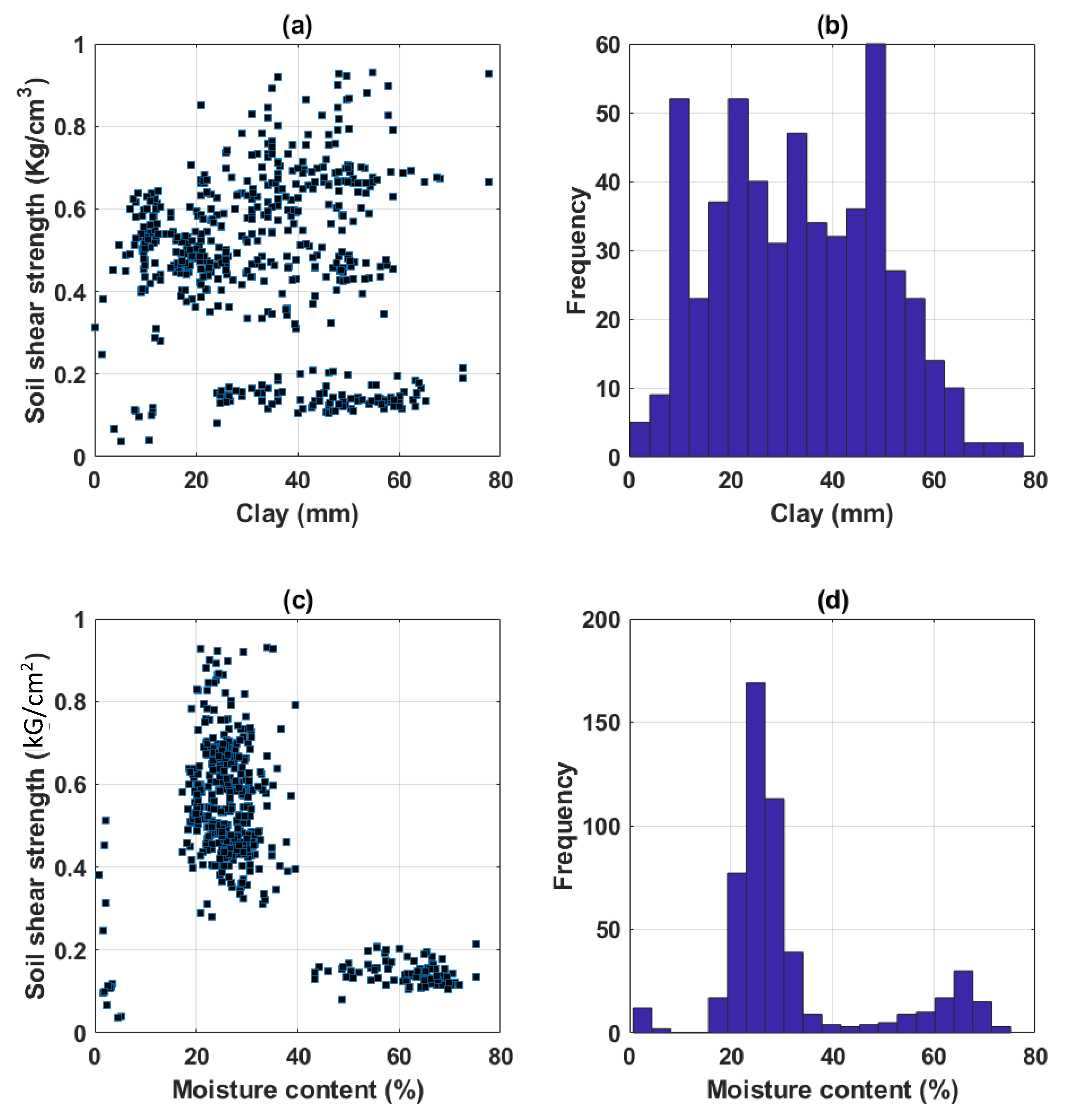
Table 1 shows the initial statistical analysis of the dataset, including the unit and coding of each variable. It is seen that statistical information, such as average, standard deviation, and quantiles of all variables, is fully exposed. For illustration purposes, Figure 2 presents the corresponding histograms of all variables used in this study, as well as the scatter plot between input variables and output response. It can be observed that the distribution of clay covered a wide range between 0 and 65 (mm), the liquid limit from 20 to 65 (%), and the plastic limit from 15 to 35 (%) with a high concentration around 20 (%). Most of the specific gravity values were in the 2.6–2.7 range, whereas the void ratio covered between the 0.5–1.0 range and a low concentration of values was around the 1.75 range. It can also be observed that there is no direct relationship between inputs and output response. Thus, it can be stated that the choice of variables in this study is relevant and suitable [12].
In order to validate the efficiency of the developed ML model, a sub-dataset calling testing part was made, exhibiting 30% (161 samples) of the total 538 configurations. It is worth noticing that such a rate of testing/training was recommended in the literature when developing ML-based models [13,14,15,16,17]. On the other hand, in order to reduce fluctuations within the dataset in training the ML model, as the variables have different ranges of values, all variables were scaled into the range of [0, 1] in order to avoid an unexpected jump in optimizing weight parameters of the models [13,18,19,20]. The scaling process of a variable x is expressed by Equation (1), and it involves two parameters, α and β, as indicated in Table 1. Precisely, α is the minimum value of the dataset and β is the maximum value.
x s c a l e d = x o r i g i n a l α β α

2.2. Extreme ML-Based Modeling

Extreme Learning Machine (ELM) is a single hidden layer feedforward neural network (SLFN). The performance of SLFN should be suitable for the system, which can be modeled for data such as critical value, weight, activation function. Therefore, higher learning can be done. In gradient-based learning approaches, all of these parameters are reiteratively modified for each appropriate value. Unlike feedforward neural networks (FNN), which are renewed based on the gradient, in the ELM process, the output weights are analytically built while the input weights are randomly chosen. For an analytic learning process, success rate increases thanks to a strong reduction of the resolution time and the error value. ELM can be introduced to choose a linear function for activating cells in a hidden layer, maybe use non-linear (such as sigmoid and sinusoidal), non-derivatized, or intermittent activation functions [21,22]. ELM algorithm can be shown in the following equations:
y ( p ) = j = 1 m α j g ( i = 1 n w i , j x i + a j )
H ( w i , j , a j , x i ) = [ g ( w 1 , 1 x 1 + a 1 ) g ( w 1 , m x m + a m ) g ( w n , 1 x n + a 1 ) g ( w n , m x m + a m ) ]
y = H α
where αi is the weights between the input layer and the hidden layer and αj is the weights between the output layer and the hidden layer, aj is the critical value of the neurons in the hidden layer, g(.) activation function. Input layer weights (wi,j) and bias (aj) are randomly selected. At the beginning of the input layer neuron number (n) and hidden-layer neuron number (m), the activation function (g(.)) is selected. To construct the ELM algorithm, the database was split into a training dataset (70% data) and the remaining data (30%) for building and validation of the ELM model.

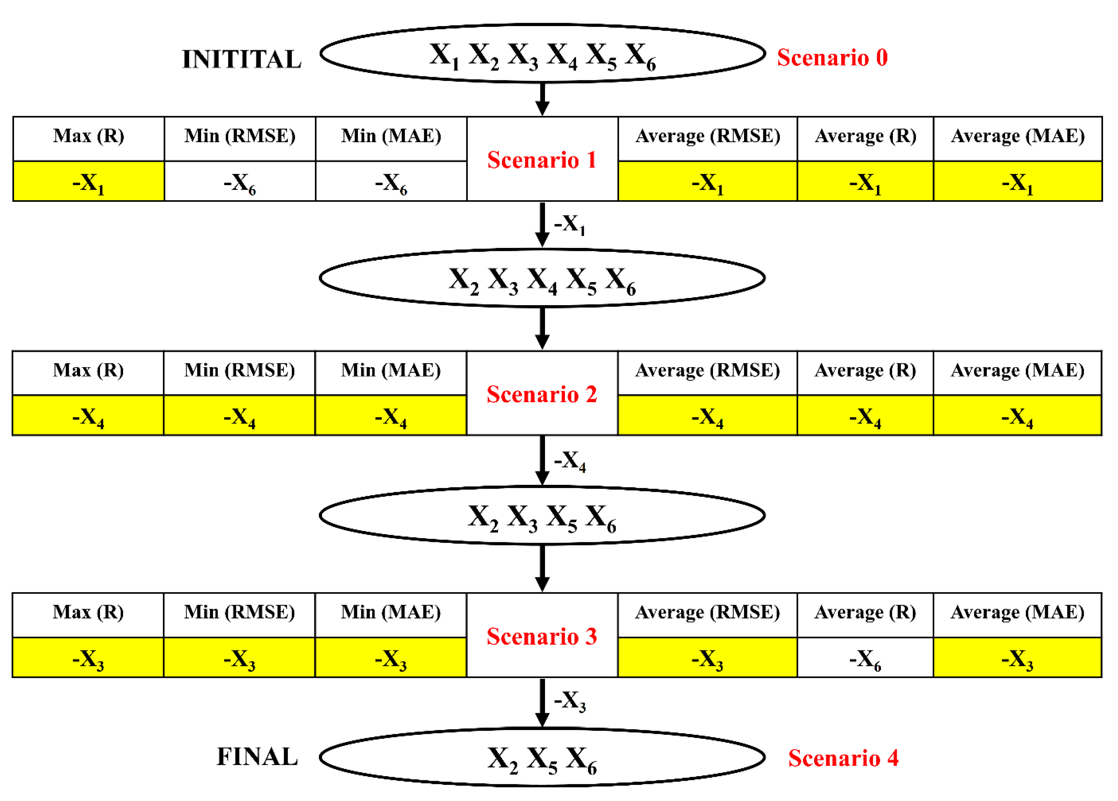
2.3. Backward Elimination-Based Sensitivity Analysis

Backward elimination, belonging to the wrapper methods, is basically the opposite of the forward selection approach [23]. Precisely, all input variables are firstly chosen, then the most unimportant of the variables are removed one by one in this case [24]. For strategic choices of the process, relative importance of an input variable can be obtained by eliminating an input variable and assessing the influence on the model to be retrained without it or by examining the effect of each input variable on the output by the sensitivity analysis method. In the filtering strategies, the least relevant candidates will be deleted repeatedly until the optimal criteria are satisfied. The process of backward elimination can be summarized in Figure 3.

2.4. Monte Carlo Simulations

Monte Carlo method is one of the most widely used techniques for propagating the input variability on the output results [25,26,27,28,29]. Regarding, for instance, the field of geotechnical engineering, Pham et al. [11] applied the Monte Carlo method for accounting variability of various content properties of soil on the prediction of its mechanical behavior under compression during a highway project. In another attempt for steel structures, the Monte Carlo technique was employed by Le et al. [15] in order to quantify the robustness of hybrid ML models for predicting the critical buckling load of structural members. For typical construction and building materials, such as concrete, many studies involving Monte Carlo technique were introduced in the literature, taking into account the variability in the input space. For instance, Wang et al. [30] quantified the size effect of random aggregates and pores on the mechanical properties of concrete. Jaskulski et al. [31] proposed a probabilistic analysis for concrete subjected to shear. So far, numerical prediction models involving Monte Carlo method could strongly explain the variation of the output results through statistical analysis.
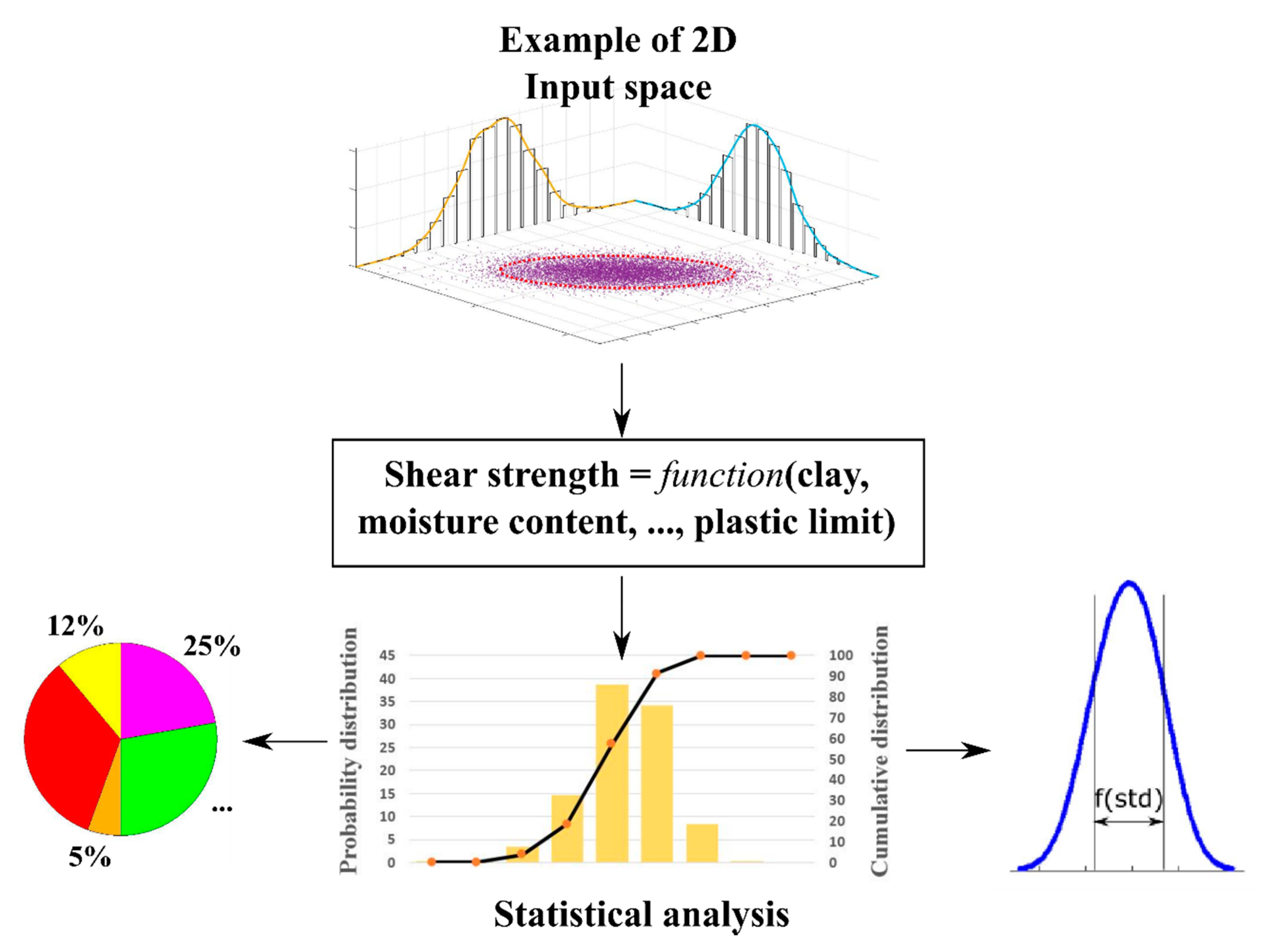
Monte Carlo method is extremely robust and efficient for calculating the propagation of the input variability on the output results, especially using ML models [11,32]. The main idea of the Monte Carlo method is to repeat realizations randomly in the input space and then calculate the corresponding output through the simulation model [33,34]. Therefore, this numerical technique exhibits a high ability in parallel computing [35,36,37,38]. A concept of using the Monte Carlo method is presented in Figure 4, involving a two-dimensional input space with a typical probability distribution.
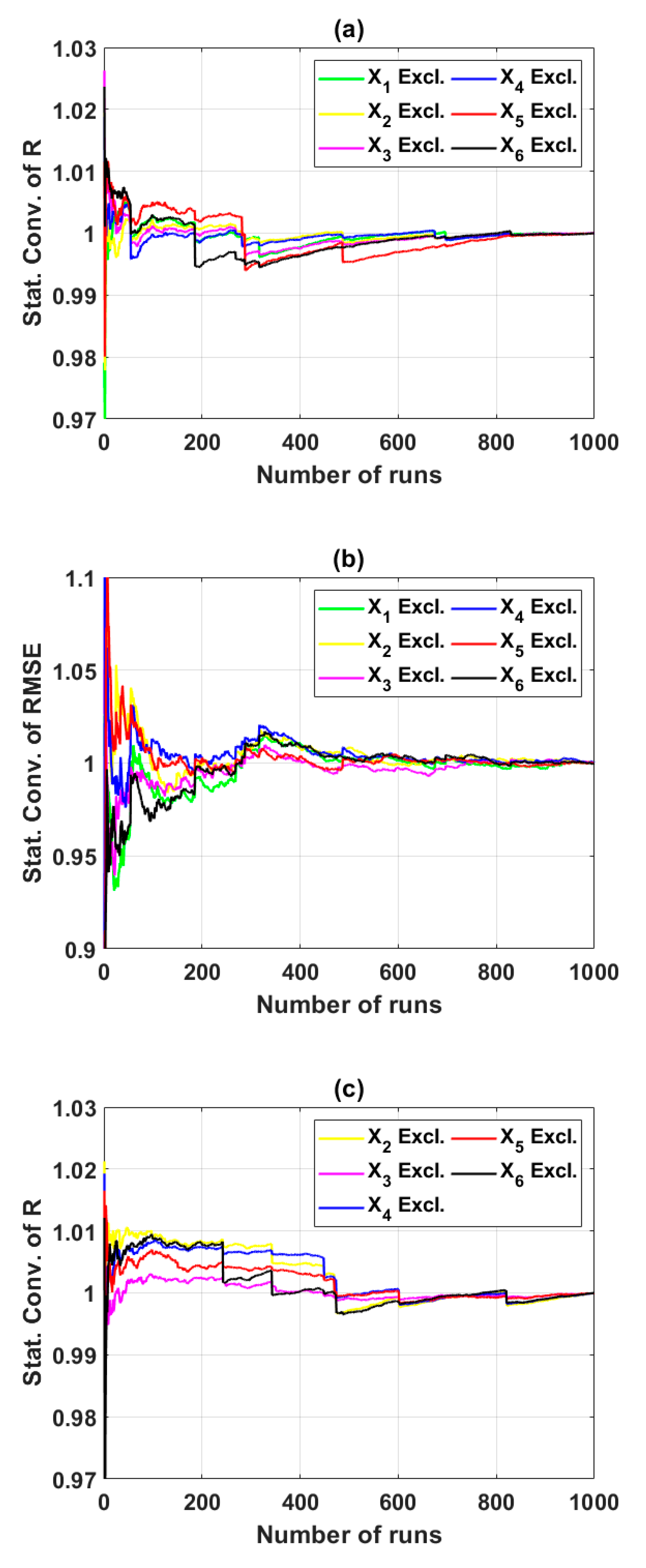
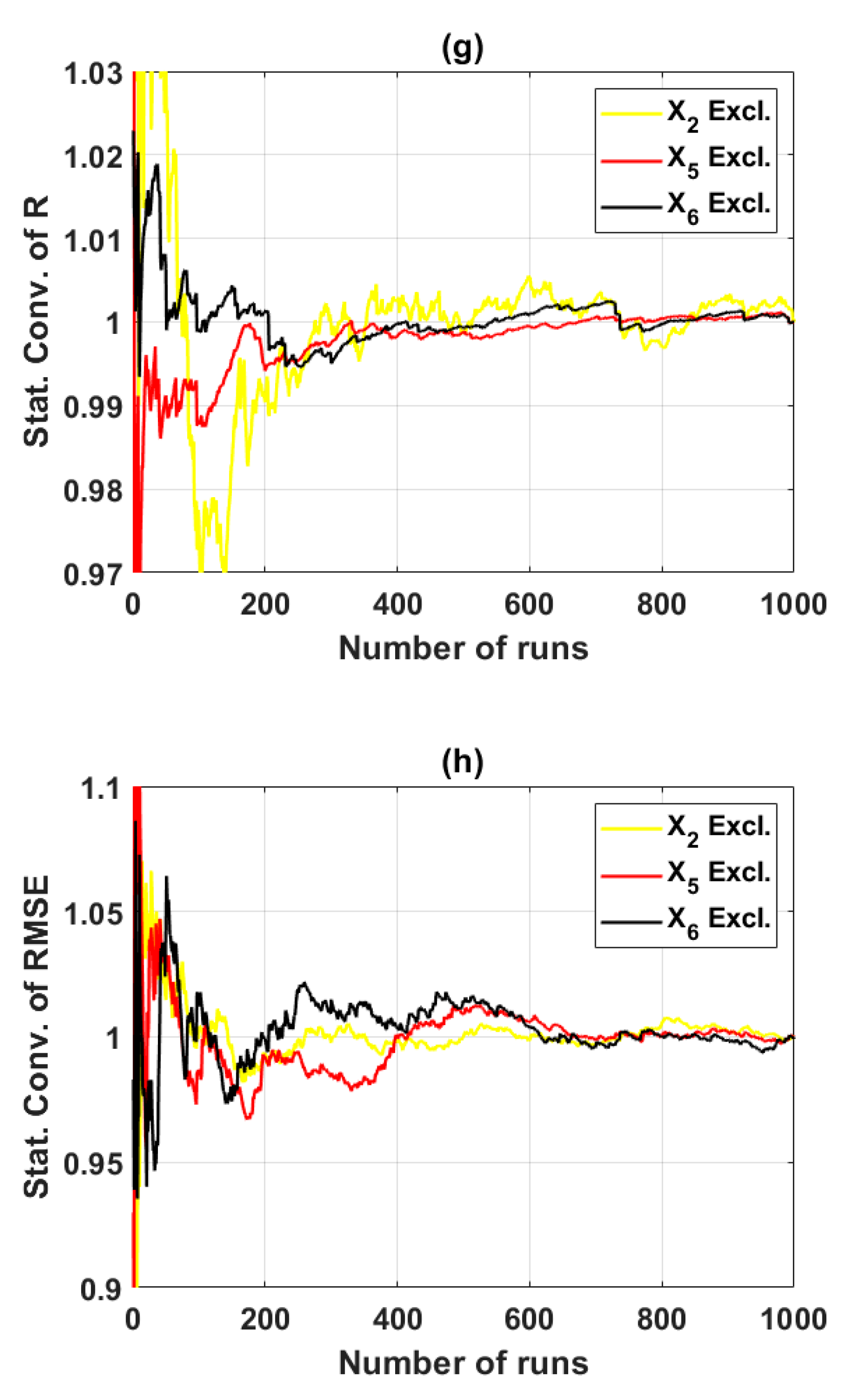
In this work, the statistical convergence of Monte Carlo simulations has been investigated using the following equation [18,32,39,40]:
f M C ( n M C ) = 1 G ¯ 1 n M C i = 1 n M C G i ,
where G ¯ is the mean value of the considered random variable G and nMC is the number of Monte Carlo runs. This convergence function provides efficient information related to the computational time, reliability results for further statistical analysis.

2.5. Performance Evaluation

To validate the predictive capability of the models, Mean Absolute Error (MAE), the Pearson correlation coefficient (R), and Root Mean Squared Error (RMSE) were selected and used, as these validation criteria are popular in evaluating the ML models. Basically, R indicates the statistical relationship between the actual values of experiments and the predicted values of the models [41]. Its absolute values range from 0 to 1 where 0 shows an inaccurate correct model and 1 indicates an accurate model. Higher R values indicate better performance of the models. RMSE indicates the average squared difference between the actual and predicted values [42]. In the case of MAE, it shows the average of absolute difference between predicted and actual values [43]. In general, RMSE and MAE show the error evaluation of the models. Thus, lower RMSE and MAE values indicate better performance of the models. Calculation of these values (R, RMSE, and MAE) can be carried out using the following equations:
MAE = i = 1 m | r i t i | m
RMSE = i = 1 m ( r i t i ) 2 m
R = i = 1 m ( r i r ) ( t i t ) i = 1 m ( r i r ) 2 i = 1 m ( t i t ) 2
where m is defined as the number of samples, ri and t are defined as the values and means of the predicted shear strength, respectively, and ti and t are the values and mean of the actual shear strength, respectively.

3. Results

3.1. Validation of ELM with Various Number of Neurons

Validation of ELM was conducted by performing 1000 simulations to each of 12 ELM architectures, where the number of neurons varied from 5 to 60 with a step of five neurons. Overall, the total number of simulations was 12,000, taking into account the random sampling index of the dataset. The results with respect to R, RMSE, and MAE are plotted in Figure 5, where the red squares represent the average values, and the blue bars show the standard deviation with respect to 1000 simulations. On the basis of average values and standard deviation of R, RMSE, and MAE, it is found that the optimal number of neurons is in the range of 15 to 25. The best performance of ELM is with 20 neurons, where the highest value of R and lowest values of RMSE and MAE were obtained. Moreover, the standard deviation of ELM using 20 neurons over 1000 random simulations is also smaller compared to other neuron options. The obtained values of average and standard deviation of RMSE are 0.1082 and 0.0231, whereas those of MAE are 0.0857, 0.0231, respectively, and those of R are 0.9218 and 0.0167, respectively. Overall, the performance of ELM is good for the prediction of shear strength of soil, and the number of 20 neurons used for training ELM was selected as an optimal choice for further investigations.

3.2. Sensitivity Analysis Using Backward Elimination and Monte Carlo Simulations

The sensitivity analysis by performing backward elimination with the help of Monte Carlo simulations is carried out in this section. A number of four scenarios (Scenarios 1 to 4), corresponding to each input space after the elimination process, was defined. The “Scenario 0” refers to the case using the initial input space without excluding any variables. The “Scenario 1” consisted of six different input spaces containing only five variables, in which each variable was excluded from the corresponding input space. For instance, six input spaces considered in this case were: (i) X2, X3, X4, X5, X6; (ii) X1, X3, X4, X5, X6; (iii) X1, X2, X4, X5, X6; (iv) X1, X2, X3, X5, X6; (v) X1, X2, X3, X4, X6; (vi) X1, X2, X3, X4, X5. Similarly, the “Scenario 2”, “Scenario 3”, and “Scenario 4” corresponded to the cases with five, four, three input spaces, respectively (Figure 3). The summarized input space and the four scenarios could be illustrated in Figure 3. The following sections are dedicated to each step of the backward elimination process.

3.2.1. Reduction of the Input Space from 6 to 5 Variables (Scenario 1)

The first step of backward elimination consists of quantifying the performance of ELM in predicting the shear strength of soil by excluding each variable successively in the input space of the database. Thus, a number of 6000 simulations (six input spaces x 1000 simulations) were performed in excluding successively from input X1 to X6. The results are plotted in Figure 6 for average values of R, RMSE, and MAE (red squares), standard deviation (blue bars) and min, max values (orange bars). Detailed values with respect to six elimination indicators are summarized in Table 2. For the sake of comparison, the discontinuous black lines represent the corresponding values of the criteria for the case of using all input variables (Scenario 0). On the basis of average values of R, it is observed that the performance of the ELM algorithm in excluding clay content (X1) slightly decreased from 0.9218 (simulation with six inputs) to 0.9203 (simulation with five inputs except for clay content). For the remaining cases (excluding from X2 to X6), the performance of ELM decreased more significantly. Similar observations were noticed taking the average values of RMSE and MAE. Indeed, it was found that excluding clay content (X1) reduced the ELM prediction performance with RMSE decrease from 0.1082 to 0.0925, and MAE decreased from 0.0857 to 0.0722 while comparing the cases of all input variables and without clay content in the input space. Besides, taking the maximum values of R or minimum value of MAE as an indicator, plastic limit (X6) was the variable to be excluded. However, taking the minimum value of RMSE as an indicator, the specific gravity (X3) was the variable to be excluded. Finally, the elimination decision was made based on the majority vote between indicators, where clay content (X1) was selected to be a less important variable compared with other variables for predicting soil shear strength.

3.2.2. Reduction of the Input Space from Five to Four Variables (Scenario 2)

The second step of backward elimination consists of the assessment of ELM capability in predicting the shear strength of soil by excluding each of the remaining inputs (X2 to X6). Thus, a number of 5000 simulations (5 input spaces × 1000 simulations) were performed. The results of average and standard deviation values of R, RMSE and MAE are displayed in Figure 7. Detailed values with respect to six indicators are summarized in Table 3. The discontinuous black lines represent the error criteria values for the case without using clay content (X1) as input variable. On the basis of average values of R, it is observed that the performance of the ELM algorithm in excluding void ratio (X4) decreased from 0.9203 (simulation with five inputs except clay content) to 0.9188 (simulation with four inputs except clay content and void ratio). For the remaining cases (excluding X2, X3, X5, and X6), the performance of ELM exhibited lower values (Table 3). Similar remarks were observed for the average values of RMSE and MAE. Indeed, it was found that excluding the void ratio made inconsiderable changes with RMSE (increase from 0.0925 to 0.0957) and MAE (increase from 0.0722 to 0.0751) with respect to the cases of all input variables without clay content as a variable. Interestingly, taking the maximum values of R, or minimum values of RMSE and MAE as indicators, the void ratio was also the variable to be excluded. The elimination at this stage revealed that void ratio (X4) is a less important variable compared with other variables (X2, X3, X5 and X6) in predicting the soil shear strength.

3.2.3. Reduction of the Input Space from Four to Three Variables (Scenario 3)

The third step of backward elimination consists of predicting the shear strength of soil by successively excluding the remaining inputs (X2, X3, X5, and X6). This induces a total number of 4000 simulations (4 input spaces × 1000 simulations) to be performed. The results of average and standard deviation values of R, RMSE, and MAE are plotted in Figure 8. Detailed simulation results with respect to six indicators are summarized in Table 4. The discontinuous black lines represent the error criteria values for the simulation without using clay content (X1) and void ratio (X4) as input variables. With respect to the average values of R, it is observed that the performance of ELM algorithm in excluding plastic limit (X6) slightly decreased from 0.9188 (simulation with four inputs without clay content and void ratio) to 0.9164 (simulation with three inputs except for clay content, void ratio, and plastic limit). On the contrary, different remarks were observed for the average values of RMSE and MAE. Precisely, it was found that excluding specific gravity made inconsiderable changes with RMSE (increase from 0.0931 to 0.0993) and MAE (increase from 0.0732 to 0.0778). More importantly, taking the maximum values of R, or minimum values of RMSE and MAE as indicators, specific gravity was the variable need to be eliminated. The backward elimination at this stage revealed that the specific gravity (X3) is less important input variable compared with other variables (X2, X5, and X6) in predicting the shear strength of soil.

3.2.4. Final Input Space with Three Variables (Scenario 4)

The final step of backward elimination in this study consists of performing the prediction by excluding one of the remaining inputs (X2, X5, and X6). At this stage, the total number of 3000 simulations (3 input spaces × 1000 simulations) was performed. The results of average and standard deviation values of R, RMSE, and MAE are plotted in Figure 9. Detailed simulation results with respect to six indicators are summarized in Table 5. The discontinuous black lines represent the error criteria values for the simulation without using clay content (X1), specific gravity (X3) and void ratio (X4) as input variables. With respect to the average values of R, it is observed that the performance of ELM algorithm in excluding plastic limit (X6) slightly decreased from 0.9138 (simulation with four inputs without clay content, specific gravity, and void ratio) to 0.8815 (simulation with two inputs moisture content and liquid limit). On the contrary, different remarks were observed for the average values of RMSE and MAE. Precisely, it was found that excluding the liquid limit made inconsiderable changes with RMSE (increase from 0.0993 to 0.1334) and MAE (increase from 0.0778 to 0.0778). On the other hand, taking the maximum values of R, or minimum values of RMSE and MAE as indicators, the plastic limit was the variable need to be eliminated. Overall, it could be considered that the plastic limit is less important than the liquid limit and moisture content in predicting the shear strength of soil, and thus, it can be concluded that moisture content is the most important factor for the prediction of the shear strength of soil.

4. Discussions

4.1. Performance of ELM in Predicting the Shear Strength of Soil

Overall, the performance of the ELM algorithm in predicting the shear strength of soil is satisfactory. From Scenarios 1 to 4, in reducing the input space from six to three variables, the accuracy of ELM was reasonably accepted. Precisely, the average values of R decreased from 0.9218 to 0.8815, those of RMSE were varied in the range of 0.1082–0.1334 and an increase of MAE values from 0.0857 to 0.1093 between Scenario 0 and Scenario 4, respectively. ELM algorithm could thus be considered as a good predictor to deal with the soil shear strength problem. Moreover, the computation time of ELM is very fast in comparison with other common ML methods such as ANN, ANFIS, or SVM [11]. For illustration purposes, one simulation using ELM in this study took only less than 0.1 seconds, which could be very efficient for massively parallel computing. The total 30,000 simulations in this study were conducted in just a few hours in an Intel Xeon E3-1505M V5 2.80GHz computer using eight processors. The reason lies in the main concept of ELM, by random initialization of the single hidden layer feedforward NN for the weights and biases [44].

4.2. Reliability of the Predicted Results by Monte Carlo Approach

The reliability of an ML algorithm, represented by the convergence of simulation results, is crucial for any analysis. Presented in the previous sections, the convergence analysis via Monte Carlo simulation is performed in order to provide additional information on the prediction capability of the ELM model. It is worth noticing that, for the sake of simplicity, only results of R and RMSE are shown in Figure 10. Overall, the R values over five simulation scenarios were converged after only 200 runs (in a 1% range compared with the average values of R), whereas smaller fluctuation can be achieved over 700 simulations in all the cases. For RMSE values, the fluctuations were observed in the 4% range compared with the corresponding average values of RMSE. More stable results were achieved when the number of simulations exceeded 800. Interestingly, in excluding the liquid limit (X5), the plastic limit (X6) or moisture content (X2) from the input space seemed to highly increase the fluctuations of the statistical analysis. This could be another confirmation to strengthen the conclusion of the backward selection feature in this study, as these three variables were considered as important. The fluctuation analysis of results was in very good agreement with the convergence analysis. Thus, performing backward elimination coupling with Monte Carlo simulation as a support decision indicator, an in-depth point of view on the importance of variables could be revealed.

4.3. Backward Elimination Criteria-Based Sensitivity Analysis

The backward elimination process, belonging to the wrapper methods, has been empirically proven that it obtains subsets with better performance than certain feature selection methods (i.e., filters methods) as the obtained subsets are evaluated by real modeling algorithms [24]. Moreover, comparing with forward selection, backward elimination finds a stronger subset of features because of the full assessment of features during the selection process [23]. Last but not least, backward elimination could reveal information not only on the importance but also the unimportance of input variables. However, selecting the criteria to remove such variables from the input space is crucial. In this study, six criteria were proposed and independently evaluated to provide useful information to the final decision. The average values of R, RMSE, or MAE could be potential candidates as they reflect the global, converged performance of the ELM algorithm over a sufficient number of simulations. It is found that, in all cases, the average values of RMSE and MAE were the reliable indicators for the elimination process. The average value of R was failed in one case (Scenario 3), similar to the minimum values of RMSE and MAE (Scenario 1).
The results show that the values of R attained negative values in several cases. This could be the reason for several sudden changes in the statistical convergence curves (Figure 9), making the average value of R not a good indicator. This is quite familiar for all ML algorithms performed with Monte Carlo simulation, as the values of R could be stable (ANFIS model in [45], SVM algorithm in [11]) or unstable (ANN algorithm in [45]). The values of RMSE and MAE were noticed to be more stable, in which extreme or outlier values were not observed. This could be because using the average values of RMSE, MAE is better than that of R. Interestingly, the maximum values of R were also found as a reliable elimination indicator in this study. In fact, choosing ML model with the highest accuracy (maximum value of R or R2) to perform further investigation is very common in the literature, for instance, in [17]. The maximum values of R or minimum values of RMSE and MAE only represented the best performance of the ELM algorithm over a certain number of Monte Carlo simulations. Even though the number of 1000 runs in each case was proven to be statistically satisfied, these values could change when increasing the number of simulations. Therefore, the use of maximum values of R or minimum values of RMSE and MAE as backward elimination indicators still needs further investigations.

4.4. Importance of Input Factors for Prediction of Soil Shear Strength

Validation of the importance of input factors for developing and applying ML models is an essential task which will help in selecting the most suitable factors used for more effective and accurate modeling and prediction. In this study, with the help of a combination approach of EML, Monte Carlo and backward elimination, the importance of input factors for prediction of soil shear strength was validated and determined (Table 6). Except for Scenario 2, the study found that the moisture content, liquid limit and plastic limit were the three most important input variables. Considering Scenarios 1 and 2, the liquid limit is more important than others, however, Scenarios 3 and 4 demonstrated that the moisture content had a stronger effect on predicting the soil shear strength than others. In general, water-related factors are the most important parameters affecting the soil shear strength and the performance of the predictive ML model. It is reasonable because water can significantly reduce the friction and link between soil particles, thus, the shear strength of less-water soil will be higher than those of more-water soil. The finding of this study is also comparative with other published studies [46,47].
The limitation of this study is that the feature interaction might be a phenomenon that slightly changed the order of importance in the present study [48]. It occurs when such feature has a little correlation with the predicted target but highly correlated when treating with another feature, so that excluding these types of features could reduce the performance of the ML algorithms [48]. With respect to the change of ML algorithms due to the elimination of one input, the readers could refer to the literature [14].

5. Conclusions

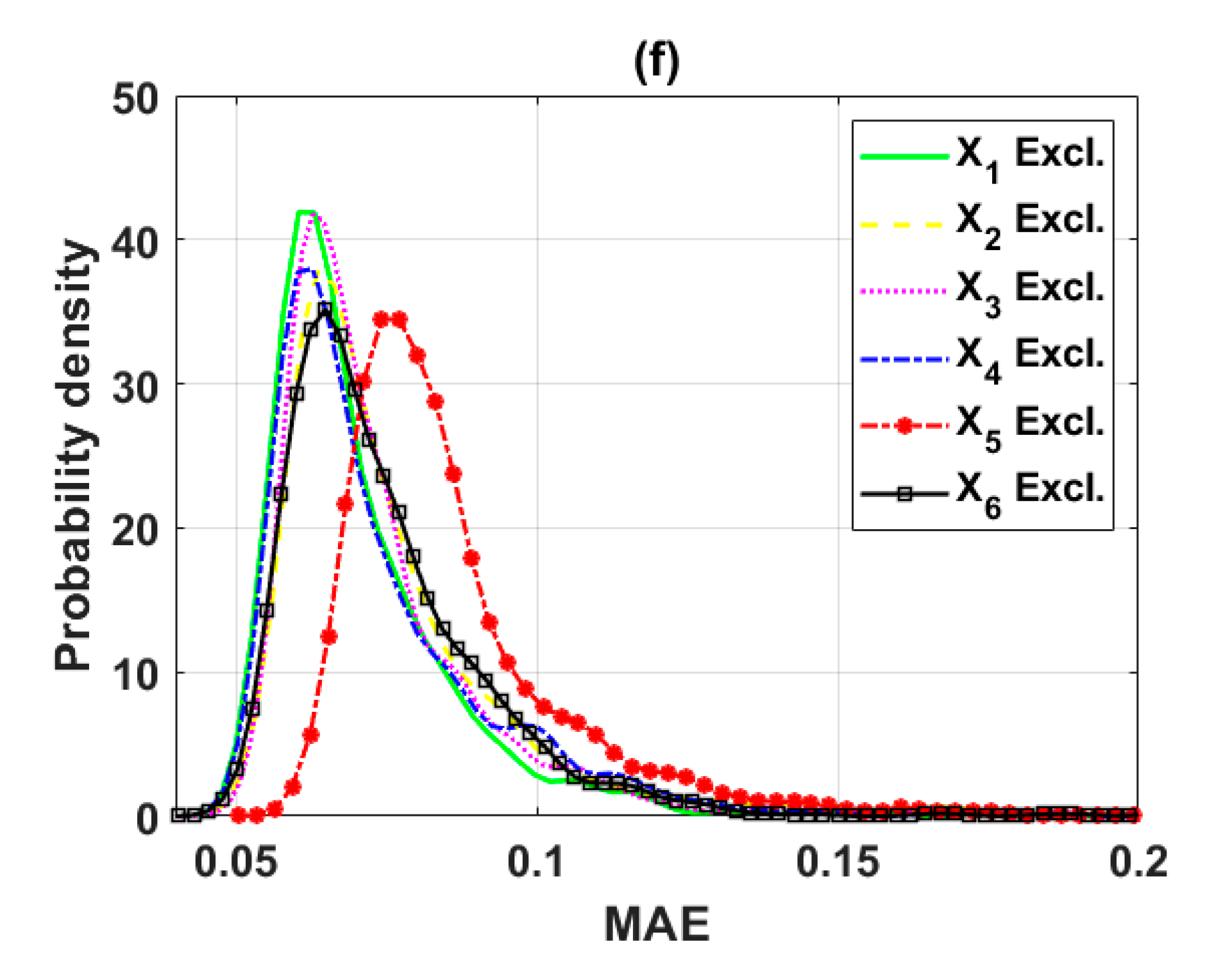
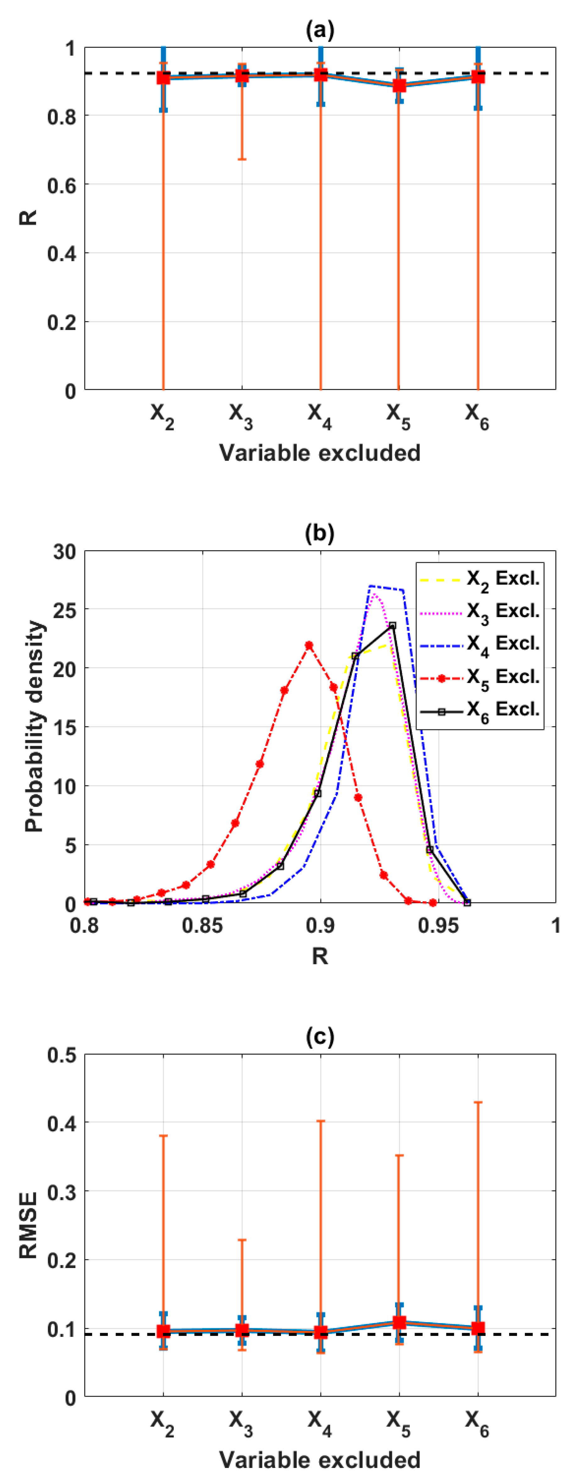
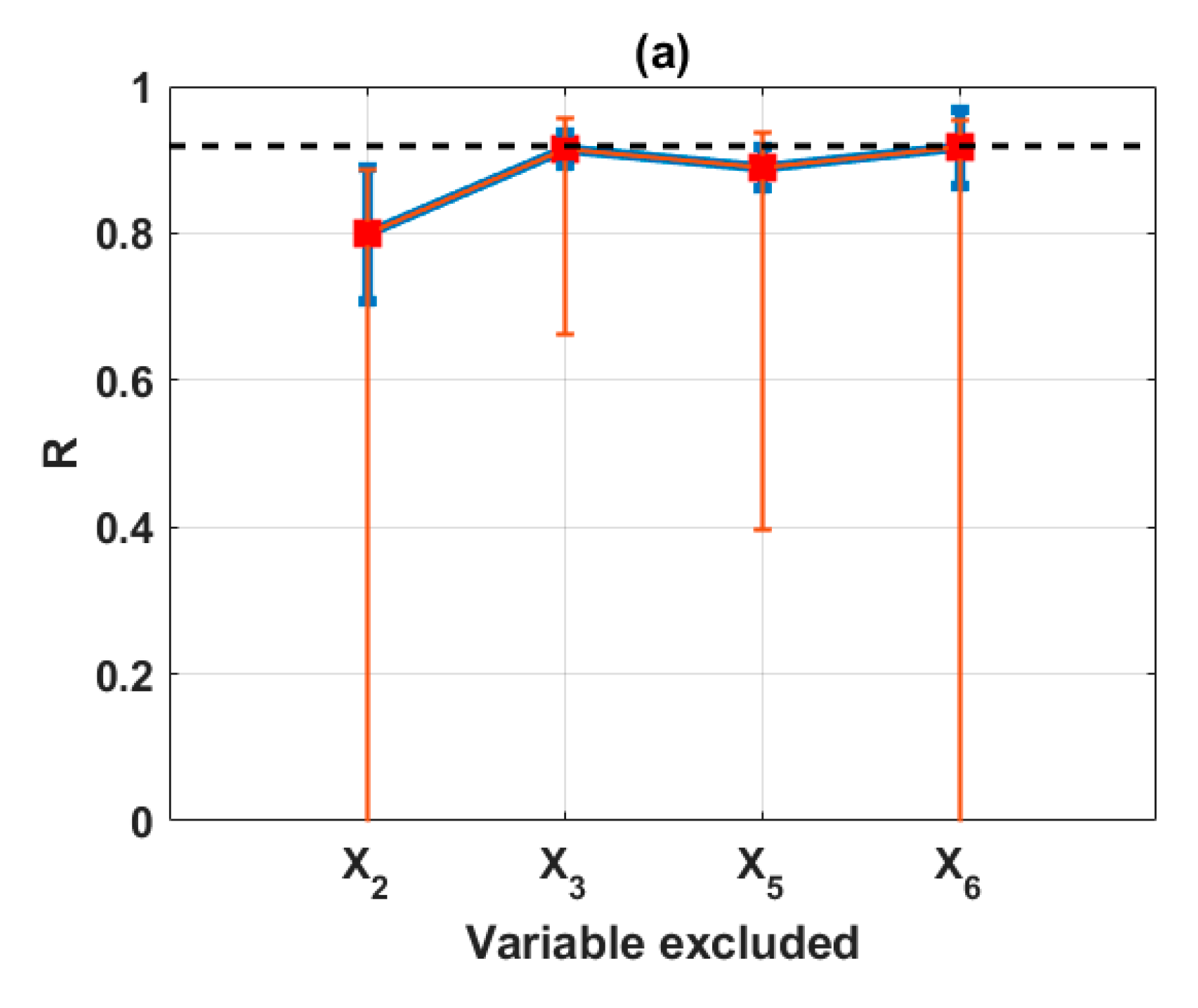
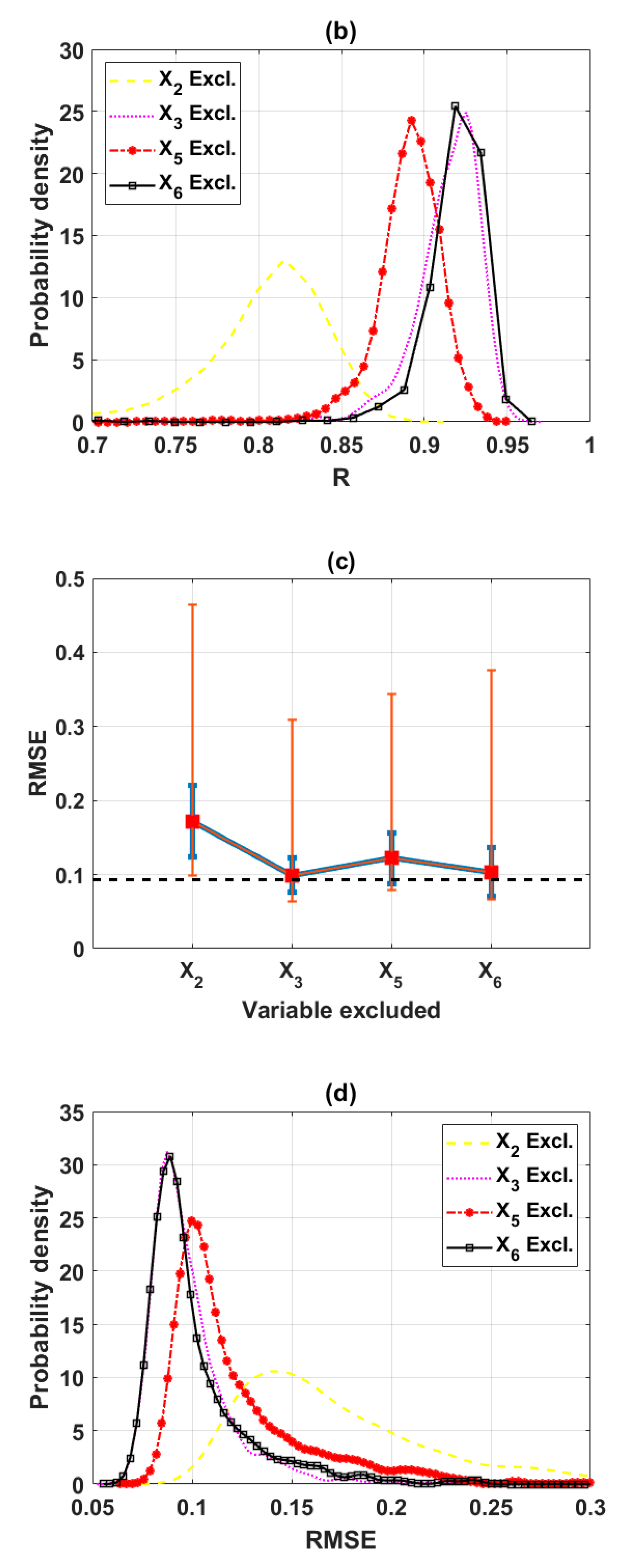
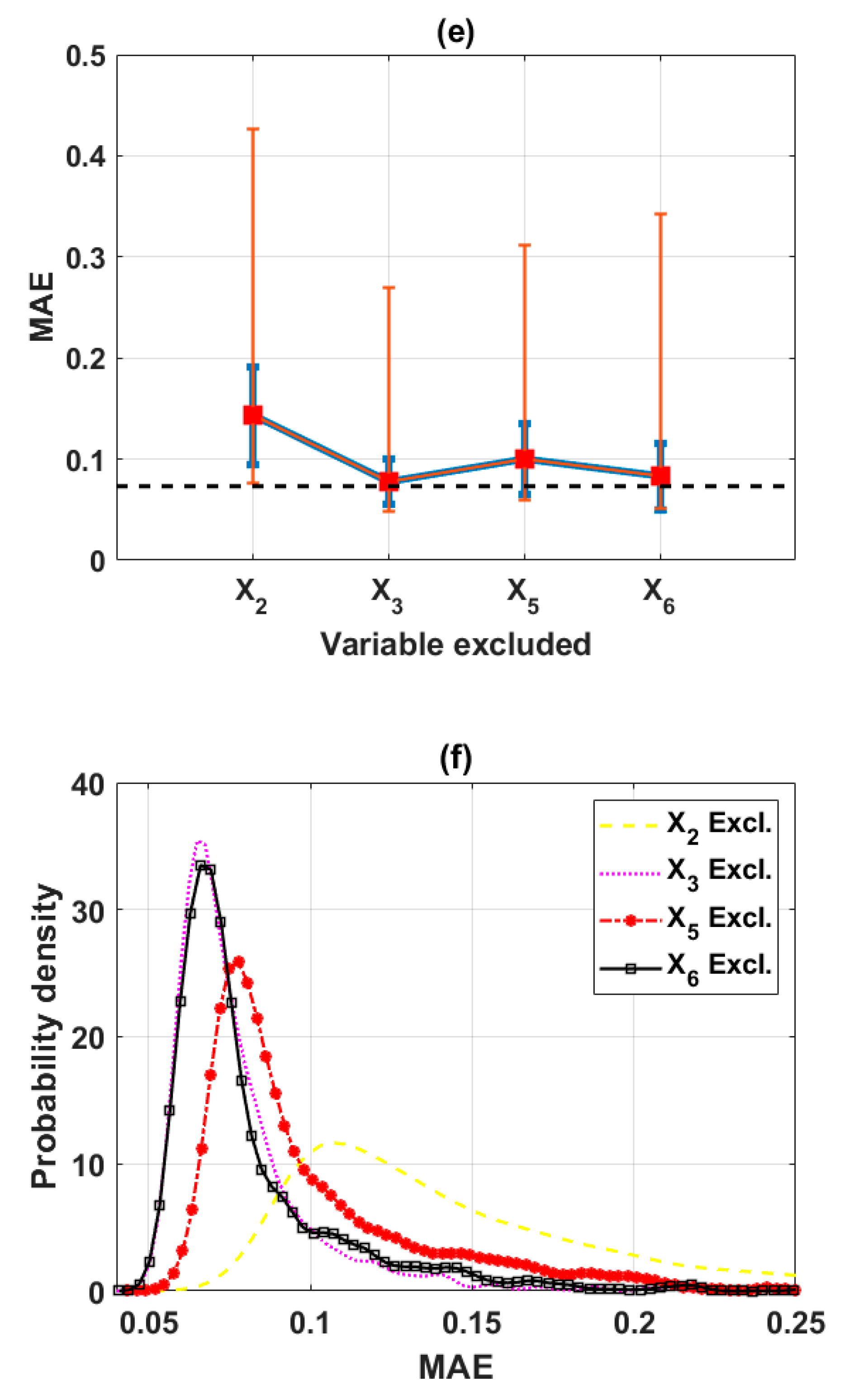
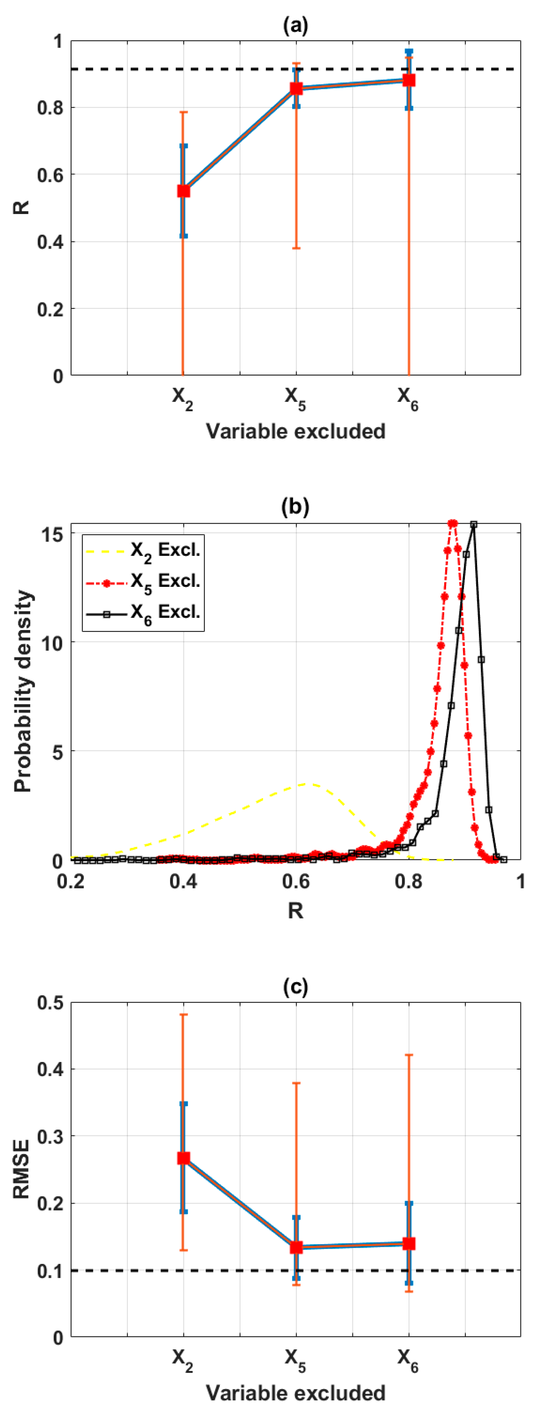
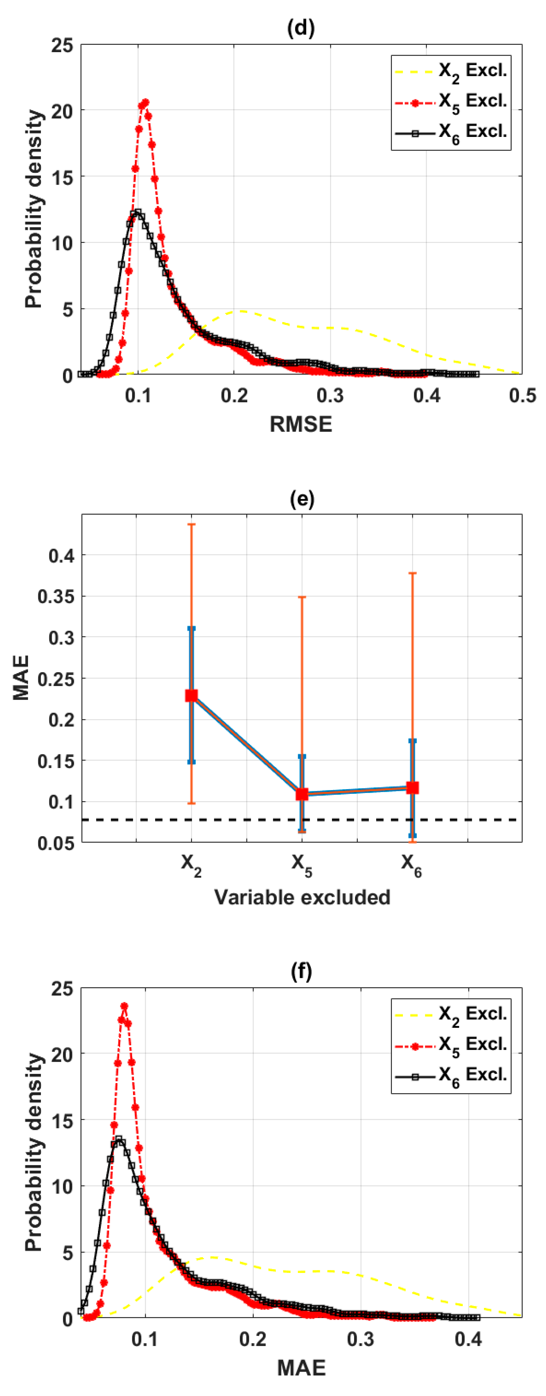
In this study, the sensitivity of an advanced ML method, namely the ELM algorithm under different feature selection scenarios for prediction of shear strength of soil was carried out. Feature backward elimination and Monte Carlo simulations were applied to evaluate the importance of factors used for the modeling. A database including input variables (moisture content (%), clay content (%), void ratio, plastic limit (%), liquid limit (%), and specific gravity) and output variable (shear strength of soil) constructed from 538 samples collected from Long Phu 1 power plant project was used for analysis. Well-known statistical indicators such as R, RMSE, and MAE were utilized to evaluate the performance of ELM algorithm. In each elimination step, the majority vote was selected to decide the variable to be excluded.
The results show that the performance of ELM is good but very different under different combinations of input factors for the prediction of shear strength of soil. The moisture content, liquid limit, and plastic limit were found as the most important variables, and other factors are less important for prediction of shear strength of soil using the ML model. This study might help to select the suitable factors for more quickly and accurately prediction of shear strength of soil using ML models.

Author Contributions

Conceptualization, B.T.P., M.D.N., N.A.-A., and H.-B.L.; methodology, H.-B.L., T.-T.L., N.A.-A., T.N.-T., and B.T.P.; validation, H.-B.L., N.A.-A., T.N.-T., and B.T.P.; formal analysis, M.D.N., T.-T.L., V.-Q.T. and H.-B.L.; data curation, V.-Q.T. and M.D.N.; writing—original draft preparation, all authors; writing—review and editing, H.-B.L., T.N.-T., N.A.-A., and B.T.P.; project administration, B.T.P. and N.A.-A.; funding acquisition, N.A.-A. All authors have read and agreed to the published version of the manuscript.

Funding

This research received no external funding.

Conflicts of Interest

The authors declare no conflict of interest.

References

  1. Tien Bui, D.; Hoang, N.-D.; Nhu, V.-H. A swarm intelligence-based machine learning approach for predicting soil shear strength for road construction: A case study at Trung Luong National Expressway Project (Vietnam). Eng. Comput. 2019, 35, 955–965. [Google Scholar] [CrossRef]
  2. Garven, E.A.; Vanapalli, S.K. Evaluation of Empirical Procedures for Predicting the Shear Strength of Unsaturated Soils. In Proceedings of the Fourth International Conference on Unsaturated Soils, Carefree, AZ, USA, 2–6 April 2006; pp. 2570–2592. [Google Scholar]
  3. Sheng, D.; Zhou, A.; Fredlund, D.G. Shear Strength Criteria for Unsaturated Soils. Geotech. Geol. Eng. 2011, 29, 145–159. [Google Scholar] [CrossRef]
  4. Vanapalli, S.K.; Fredlund, D.G. Comparison of Different Procedures to Predict Unsaturated Soil Shear Strength. In Advances in Unsaturated Geotechnics; American Society of Civil Engineers: Reston, VA, USA, 2000; pp. 195–209. [Google Scholar]
  5. Al Aqtash, U.; Bandini, P. Prediction of unsaturated shear strength of an adobe soil from the soil–water characteristic curve. Constr. Build. Mater. 2015, 98, 892–899. [Google Scholar] [CrossRef]
  6. Pham, B.T.; Son, L.H.; Hoang, T.-A.; Nguyen, D.-M.; Tien Bui, D. Prediction of shear strength of soft soil using machine learning methods. CATENA 2018, 166, 181–191. [Google Scholar] [CrossRef]
  7. Moayedi, H.; Tien Bui, D.; Dounis, A.; Kok Foong, L.; Kalantar, B. Novel Nature-Inspired Hybrids of Neural Computing for Estimating Soil Shear Strength. Appl. Sci. 2019, 9, 4643. [Google Scholar] [CrossRef] [Green Version]
  8. Nhu, V.-H.; Hoang, N.-D.; Duong, V.-B.; Vu, H.-D.; Tien Bui, D. A hybrid computational intelligence approach for predicting soil shear strength for urban housing construction: A case study at Vinhomes Imperia project, Hai Phong city (Vietnam). Eng. Comput. 2019. [Google Scholar] [CrossRef]
  9. Das, S.; Samui, P.; Khan, S.; Sivakugan, N. Machine learning techniques applied to prediction of residual strength of clay. Open Geosci. 2011, 3, 449–461. [Google Scholar] [CrossRef]
  10. Nguyen, M.D.; Pham, B.T.; Tuyen, T.T.; Hai Yen, H.P.; Prakash, I.; Vu, T.T.; Chapi, K.; Shirzadi, A.; Shahabi, H.; Dou, J.; et al. Development of an Artificial Intelligence Approach for Prediction of Consolidation Coefficient of Soft Soil: A Sensitivity Analysis. Open Constr. Build. Technol. J. 2019, 13, 178–188. [Google Scholar] [CrossRef]
  11. Pham, B.T.; Nguyen, M.D.; Dao, D.V.; Prakash, I.; Ly, H.-B.; Le, T.-T.; Ho, L.S.; Nguyen, K.T.; Ngo, T.Q.; Hoang, V.; et al. Development of artificial intelligence models for the prediction of Compression Coefficient of soil: An application of Monte Carlo sensitivity analysis. Sci. Total Environ. 2019, 679, 172–184. [Google Scholar] [CrossRef]
  12. Asteris, P.G.; Ashrafian, A.; Rezaie-Balf, M. Prediction of the compressive strength of self-compacting concrete using surrogate models. Comput. Concr. 2019, 24, 137–150. [Google Scholar]
  13. Qi, C.; Ly, H.-B.; Chen, Q.; Le, T.-T.; Le, V.M.; Pham, B.T. Flocculation-dewatering prediction of fine mineral tailings using a hybrid machine learning approach. Chemosphere 2019, 244, 125450. [Google Scholar] [CrossRef]
  14. Ly, H.-B.; Monteiro, E.; Le, T.-T.; Le, V.M.; Dal, M.; Regnier, G.; Pham, B.T. Prediction and Sensitivity Analysis of Bubble Dissolution Time in 3D Selective Laser Sintering Using Ensemble Decision Trees. Materials 2019, 12, 1544. [Google Scholar] [CrossRef] [Green Version]
  15. Le, L.M.; Ly, H.-B.; Pham, B.T.; Le, V.M.; Pham, T.A.; Nguyen, D.-H.; Tran, X.-T.; Le, T.-T. Hybrid Artificial Intelligence Approaches for Predicting Buckling Damage of Steel Columns Under Axial Compression. Materials 2019, 12, 1670. [Google Scholar] [CrossRef] [PubMed] [Green Version]
  16. Khosravi, K.; Shahabi, H.; Pham, B.T.; Adamawoski, J.; Shirzadi, A.; Pradhan, B.; Dou, J.; Ly, H.-B.; Gróf, G.; Ho, H.L. A Comparative Assessment of Flood Susceptibility Modeling Using Multi-Criteria Decision-Making Analysis and Machine Learning Methods. J. Hydrol. 2019, 573, 311–323. [Google Scholar] [CrossRef]
  17. Qi, C.; Tang, X.; Dong, X.; Chen, Q.; Fourie, A.; Liu, E. Towards Intelligent Mining for Backfill: A genetic programming-based method for strength forecasting of cemented paste backfill. Miner. Eng. 2019, 133, 69–79. [Google Scholar] [CrossRef]
  18. Ly, H.-B.; Le, L.M.; Phi, L.V.; Phan, V.-H.; Tran, V.Q.; Pham, B.T.; Le, T.-T.; Derrible, S. Development of an AI Model to Measure Traffic Air Pollution from Multisensor and Weather Data. Sensors 2019, 19, 4941. [Google Scholar] [CrossRef] [Green Version]
  19. Pham, B.T.; Jaafari, A.; Prakash, I.; Singh, S.K.; Quoc, N.K.; Bui, D.T. Hybrid computational intelligence models for groundwater potential mapping. CATENA 2019, 182, 104101. [Google Scholar] [CrossRef]
  20. Ly, H.-B.; Le, L.M.; Duong, H.T.; Nguyen, T.C.; Pham, T.A.; Le, T.-T.; Le, V.M.; Nguyen-Ngoc, L.; Pham, B.T. Hybrid Artificial Intelligence Approaches for Predicting Critical Buckling Load of Structural Members under Compression Considering the Influence of Initial Geometric Imperfections. Appl. Sci. 2019, 9, 2258. [Google Scholar] [CrossRef] [Green Version]
  21. Huang, G.-B.; Zhu, Q.-Y.; Siew, C.-K. Extreme learning machine: A new learning scheme of feedforward neural networks. In Proceedings of the 2004 IEEE International Joint Conference on Neural Networks (IEEE Cat. No.04CH37541), Budapest, Hungary, 25–29 July 2004; Volume 2, pp. 985–990. [Google Scholar]
  22. Huang, G.-B.; Zhu, Q.-Y.; Siew, C.-K. Extreme learning machine: Theory and applications. Neurocomputing 2006, 70, 489–501. [Google Scholar] [CrossRef]
  23. Kumar, V.; Minz, S. Feature selection: A literature review. Smart Comput. Rev. 2014, 4, 211–229. [Google Scholar] [CrossRef]
  24. Jović, A.; Brkić, K.; Bogunović, N. A review of feature selection methods with applications. In Proceedings of the 2015 38th International Convention on Information and Communication Technology, Electronics and Microelectronics (MIPRO), Opatija, Croatia, 25–29 May 2015; pp. 1200–1205. [Google Scholar]
  25. Christian, S. (Ed.) Stochastic Models of Uncertainties in Computational Mechanics; Amer Society of Civil Engineers: Reston, VA, USA, 2012; ISBN 978-0-7844-1223-7. [Google Scholar]
  26. Nguyen, H.-L.; Pham, B.T.; Son, L.H.; Thang, N.T.; Ly, H.-B.; Le, T.-T.; Ho, L.S.; Le, T.-H.; Tien Bui, D. Adaptive Network Based Fuzzy Inference System with Meta-Heuristic Optimizations for International Roughness Index Prediction. Appl. Sci. 2019, 9, 4715. [Google Scholar] [CrossRef] [Green Version]
  27. Nguyen, H.-L.; Le, T.-H.; Pham, C.-T.; Le, T.-T.; Ho, L.S.; Le, V.M.; Pham, B.T.; Ly, H.-B. Development of Hybrid Artificial Intelligence Approaches and a Support Vector Machine Algorithm for Predicting the Marshall Parameters of Stone Matrix Asphalt. Appl. Sci. 2019, 9, 3172. [Google Scholar] [CrossRef] [Green Version]
  28. Guilleminot, J.; Dolbow, J.E. Data-driven enhancement of fracture paths in random composites. Mech. Res. Commun. 2020, 103, 103443. [Google Scholar] [CrossRef]
  29. Wang, H.; Guilleminot, J.; Soize, C. Modeling uncertainties in molecular dynamics simulations using a stochastic reduced-order basis. Comput. Methods Appl. Mech. Eng. 2019, 354, 37–55. [Google Scholar] [CrossRef] [Green Version]
  30. Wang, X.; Yang, Z.; Jivkov, A.P. Monte Carlo simulations of mesoscale fracture of concrete with random aggregates and pores: A size effect study. Constr. Build. Mater. 2015, 80, 262–272. [Google Scholar] [CrossRef]
  31. Jaskulski, R.; Wiliński, P. Probabilistic Analysis of Shear Resistance Assured by Concrete Compression. Proced. Eng. 2017, 172, 449–456. [Google Scholar] [CrossRef]
  32. Ly, H.-B.; Desceliers, C.; Le, L.M.; Le, T.-T.; Pham, B.T.; Nguyen-Ngoc, L.; Doan, V.T.; Le, M. Quantification of Uncertainties on the Critical Buckling Load of Columns under Axial Compression with Uncertain Random Materials. Materials 2019, 12, 1828. [Google Scholar] [CrossRef] [Green Version]
  33. Mordechai, S. Applications of Monte Carlo Method in Science and Engineering; IntechOpen: London, UK, 2011; ISBN 978-953-307-691-1. [Google Scholar]
  34. Guilleminot, J.; Soize, C. Generalized stochastic approach for constitutive equation in linear elasticity: A random matrix model. Int. J. Numer. Methods Eng. 2012, 90, 613–635. [Google Scholar] [CrossRef] [Green Version]
  35. Soize, C. Uncertainty Quantification: An Accelerated Course with Advanced Applications in Computational Engineering; Interdisciplinary Applied Mathematics; Springer International Publishing: Berlin, Germany, 2017; ISBN 978-3-319-54338-3. [Google Scholar]
  36. Cunha, A.; Nasser, R.; Sampaio, R.; Lopes, H.; Breitman, K. Uncertainty quantification through the Monte Carlo method in a cloud computing setting. Comput. Phys. Commun. 2014, 185, 1355–1363. [Google Scholar] [CrossRef] [Green Version]
  37. Le, T.T.; Guilleminot, J.; Soize, C. Stochastic continuum modeling of random interphases from atomistic simulations. Application to a polymer nanocomposite. Comput. Methods Appl. Mech. Eng. 2016, 303, 430–449. [Google Scholar] [CrossRef] [Green Version]
  38. Soize, C.; Desceliers, C.; Guilleminot, J.; Le, T.T.; Nguyen, M.T.; Perrin, G.; Allain, J.M.; Gharbi, H.; Duhamel, D.; Funfschilling, C. Stochastic representations and statistical inverse identification for uncertainty quantification in computational mechanics. In Proceedings of the Uncecomp 2015 1st Eccomas Thematic Conference on Uncertainty Quantification in Computational Sciences and Engineering, Crete Island, Greece, 25–27 May 2015; pp. 1–26. [Google Scholar]
  39. Guilleminot, J.; Le, T.T.; Soize, C. Stochastic framework for modeling the linear apparent behavior of complex materials: Application to random porous materials with interphases. Acta Mech. Sin. 2013, 29, 773–782. [Google Scholar] [CrossRef] [Green Version]
  40. Staber, B.; Guilleminot, J.; Soize, C.; Michopoulos, J.; Iliopoulos, A. Stochastic modeling and identification of a hyperelastic constitutive model for laminated composites. Comput. Methods Appl. Mech. Eng. 2019, 347, 425–444. [Google Scholar] [CrossRef] [Green Version]
  41. Dao, D.V.; Trinh, S.H.; Ly, H.-B.; Pham, B.T. Prediction of Compressive Strength of Geopolymer Concrete Using Entirely Steel Slag Aggregates: Novel Hybrid Artificial Intelligence Approaches. Appl. Sci. 2019, 9, 1113. [Google Scholar] [CrossRef] [Green Version]
  42. Ly, H.-B.; Pham, B.T.; Dao, D.V.; Le, V.M.; Le, L.M.; Le, T.-T. Improvement of ANFIS Model for Prediction of Compressive Strength of Manufactured Sand Concrete. Appl. Sci. 2019, 9, 3841. [Google Scholar] [CrossRef] [Green Version]
  43. Ly, H.-B.; Le, T.-T.; Le, L.M.; Tran, V.Q.; Le, V.M.; Vu, H.-L.T.; Nguyen, Q.H.; Pham, B.T. Development of Hybrid Machine Learning Models for Predicting the Critical Buckling Load of I-Shaped Cellular Beams. Appl. Sci. 2019, 9, 5458. [Google Scholar] [CrossRef] [Green Version]
  44. Miche, Y.; Van Heeswijk, M.; Bas, P.; Simula, O.; Lendasse, A. TROP-ELM: A double-regularized ELM using LARS and Tikhonov regularization. Neurocomputing 2011, 74, 2413–2421. [Google Scholar] [CrossRef]
  45. Dao, D.V.; Ly, H.-B.; Trinh, S.H.; Le, T.-T.; Pham, B.T. Artificial Intelligence Approaches for Prediction of Compressive Strength of Geopolymer Concrete. Materials 2019, 12, 983. [Google Scholar] [CrossRef] [Green Version]
  46. Cokca, E.; Erol, O.; Armangil, F. Effects of compaction moisture content on the shear strength of an unsaturated clay. Geotech. Geol. Eng. 2004, 22, 285. [Google Scholar] [CrossRef]
  47. Spoor, G.; Godwin, R.J. Soil Deformation and Shear Strength Characteristics of Some Clay Soils at Different Moisture Contents. J. Soil Sci. 1979, 30, 483–498. [Google Scholar] [CrossRef]
  48. Calder, M.; Kolberg, M.; Magill, E.H.; Reiff-Marganiec, S. Feature interaction: A critical review and considered forecast. Comput. Netw. 2003, 41, 115–141. [Google Scholar] [CrossRef] [Green Version]
Figure 1. Location of the study site: Long Phu 1 power plant (https://www.power-technology.com/projects/long-phu-1-thermal-power-plant-soc-trang-province/).
Sustainability 12 02339 g001
Figure 2. Histograms of the parameters used in this study and correlation graphs with the output: (a,b) Clay, (c,d) moisture content, (e,f) specific gravity, (g,h) void ratio, (i,j) liquid limit, (k,l) plastic limit, and (m) shear strength of soil.
Sustainability 12 02339 g002aSustainability 12 02339 g002bSustainability 12 02339 g002c
Figure 3. The process of backward elimination supported by Monte Carlo simulations in this study. (Correlation coefficient (R); Root mean squared error (RMSE); Mean absolute error (MAE)).
Sustainability 12 02339 g003
Figure 4. Schematization of using Monte Carlo for statistical analysis purposes.
Sustainability 12 02339 g004
Figure 5. Validation of ELM algorithm with various numbers of neurons using different validation criteria: (a) R, (b) RMSE, and (c) MAE.
Sustainability 12 02339 g005
Figure 6. ELM performance with a reduction of the input space from six to five variables (Scenario 1) for the case of (a) R; (b) probability density function of R; (c) RMSE; (d) probability density function of RMSE; (e) MAE; and (f) probability density function of MAE.
Sustainability 12 02339 g006aSustainability 12 02339 g006bSustainability 12 02339 g006c
Figure 7. ELM performance with reduction of the input space from five to four variables (Scenario 2) for the case of (a) R; (b) probability density function of R; (c) RMSE; (d) probability density function of RMSE; (e) MAE; and (f) probability density function of MAE.
Sustainability 12 02339 g007aSustainability 12 02339 g007b
Figure 8. ELM performance with reduction of the input space from four to three variables (Scenario 3) for the case of (a) R; (b) probability density function of R; (c) RMSE; (d) probability density function of RMSE; (e) MAE; and (f) probability density function of MAE.
Sustainability 12 02339 g008aSustainability 12 02339 g008bSustainability 12 02339 g008c
Figure 9. ELM performance with a reduction of the input space with three variables (Scenario 4) for the case of (a) R; (b) probability density function of R; (c) RMSE; (d) probability density function of RMSE; (e) MAE; and (f) probability density function of MAE.
Sustainability 12 02339 g009aSustainability 12 02339 g009b
Figure 10. Statistical convergence analysis using backward elimination and 1000 Monte Carlo simulations for four scenarios in this study: (a) R for Scenario 1; (b) RMSE for Scenario 1; (c) R for Scenario 2; (d) RMSE for Scenario 2; (e) R for Scenario 3; (f) RMSE for Scenario 3; (g) R for Scenario 4; (h) RMSE for Scenario 4.
Sustainability 12 02339 g010aSustainability 12 02339 g010bSustainability 12 02339 g010c
Table 1. Initial analysis of data used in this study.
ParameterClayMoisture ContentSpecific GravityVoid RatioLiquid LimitPlastic LimitSoil Shear Strength
Unitmm%--%%kG/cm2
CodingX1X2X3X4X5X6Y
Min (α)0.20000.72000.01000.02100.70000.60000.0368
Average33.246731.83362.61420.914242.364922.16780.4791
Median33.200026.55002.69000.787042.500021.40000.4964
Max (β)77.600075.14002.75002.089074.900041.00000.9307
SD*16.138815.26710.42710.393513.26356.13760.2036
Q2520.700023.61002.67000.709033.500018.70000.3978
Q5033.200026.55002.69000.787042.500021.40000.4964
Q7547.400030.97002.71000.885050.400024.30000.6287
SD* = Standard deviation.
Table 2. ELM performance while reducing the input space from six to five input variables.
ExcludedX1X2X3X4X5X6FullDecide
Mean (R)0.92030.91210.91360.91910.88580.91670.9218X1
Max (R)0.95810.95040.95020.96040.93020.9552-X4
Mean (RMSE)0.09250.09680.09440.09410.10800.09610.1082X1
Min (RMSE)0.06750.06620.06390.06410.07970.0652-X3
Mean (MAE)0.07220.07620.07400.07430.08670.07530.0857X1
Min (MAE)0.05060.05000.04890.05020.06010.0482-X6
Table 3. ELM performance while reducing the input space from five to four input variables.
ExcludedX2X3X4X5X6FullDecide
Mean (R)0.90890.91490.91880.88680.91130.9203X4
Max (R)0.95280.95030.95330.93330.9503-X4
Mean (RMSE)0.09570.09690.09310.10830.10020.0925X4
Min (RMSE)0.06940.06830.06440.07720.0650-X4
Mean (MAE)0.07510.07600.07320.08610.07930.0722X4
Min (MAE)0.05080.05070.04950.05930.0511-X4
Table 4. ELM performance while reducing the input space from four to three input variables.
ExcludedX2X3X5X6FullDecide
Mean (R)0.79850.91380.88970.91640.9188X6
Max (R)0.88640.95740.93600.9535-X3
Mean (RMSE)0.17220.09930.12190.10310.0931X3
Min (RMSE)0.09900.06330.07920.0670-X3
Mean (MAE)0.14290.07780.10020.08270.0732X3
Min (MAE)0.07580.04800.05910.0516-X3
Table 5. ELM performance while reducing the input space from four to three input variables.
ExcludedX2X5X6FullDecide
Mean(R)0.54990.85710.88150.9138X6
Max(R)0.78510.93220.9481-X6
Mean(RMSE)0.26730.13340.13970.0993X5
Min(RMSE)0.12960.07820.0684-X6
Mean(MAE)0.22910.10930.11620.0778X5
Min(MAE)0.09790.06270.0509-X6
Table 6. Order of importance over four scenarios in this study.
Order of Importance123456
Scenario 1X1X4X3X6X2X5
Scenario 2X4X2X3X6X5-
Scenario 3X3X6X5X2--
Scenario 4X5X6X2---

