Article

Study of the Effects of Vent Configuration on Mono-Span Greenhouse Ventilation Using Computational Fluid Dynamics

1
Department of Engineering, University of Exeter, Exeter EX4 4QF, UK
2
Water and Water structures Engineering Department, Faculty of Engineering, Zagazig University, Zagaizg 44519, Egypt
*
Author to whom correspondence should be addressed.
Sustainability 2020, 12(3), 986; https://doi.org/10.3390/su12030986
Submission received: 7 January 2020 / Revised: 23 January 2020 / Accepted: 28 January 2020 / Published: 29 January 2020
(This article belongs to the Special Issue Sustainability in Urban Horticulture)

Abstract

:
The rise in the human population, its density and scarcity of resources require cost-effective solutions for sustainable energy and water resources. Smart and sustainable agriculture is one important factor for future green cities to tackle climate change as a cost-effective solution to save energy and water. However, greenhouses (GH) require consistent ventilation due to their internal temperatures, and this can be an energy-intensive operation. Therefore, it is necessary to analyse the potential factors involved. In this study, the effect of vent configuration of a mono-span greenhouse with roof and side vents at low wind speeds was investigated using computational fluid dynamics (CFD). The validated simulations were then performed on different models to analyse the effects of the vents’ locations on the ventilation requirements. The side vents were found to contribute most to the ventilation. The position of the side vent was found to affect the convection loop in the greenhouse and the air velocity at the plant level. The humidity was shown to be highest under the windward side vent. The roof vent was found to affect the temperature and air velocity in the roof of the greenhouse but had very little effect on the distributions at the plant level.

1. Introduction

A greenhouse (GH) is an indoor production facility with a transparent cover, used to grow plants under ideal conditions, as it allows good control of the external conditions in which the plants are grown, such as temperature, air velocity and flow pattern, ventilation rate, humidity and CO2 concentration. Traditionally, GHs are used in cold climates to protect crops from the wind and increase the internal temperature, to grow crops that would usually not be able to grow in cold climates. However, recently, smart GHs are also being used in warm regions to provide shading and remove excess heat and humidity, so that plants can be grown more effectively. This is especially important in the Middle East and North African (MENA) region, with scant water resources [1,2]. Furthermore, high temperatures with intense solar energy and low humidity cause open field agriculture to be less economical [2], while available intense solar energy provided situations for implementing sustainable technologies [3,4,5,6,7]. By using GHs, the water demands for irrigation can be reduced by up to 90% for countries with water stresses [2]. Linked to this, many countries in the MENA region have deployed desalination technologies for irrigation [8]. Since the temperature inside the GH reaches to a certain level, ventilation, shading and also the cooling technologies are important to provide suitable temperature for the plants’ growth [9]. While water demands can be controlled in the GHs, the ventilation needs to be analysed experimentally and/or computationally to enable the design of cost-effective smart ventilation technologies. Computational Fluid Dynamics (CFD) can simulate the GH micro-climate status and investigate the arrangements of ventilators based on the air velocities. Generally, after development, a CFD model is verified against experimental results, to ensure that CFD results are accurate and simulate physical GHs in the same conditions. Experimental approaches have also been deployed in previous studies to analyse the ventilation requirements on real GHs [10,11] using a tracer gas technique [12]. Some others analysed the distribution of temperature and velocity contours in the GHs by deploying thermocouples placed at certain predefined points to measure the air velocity and temperature [13]. Bartzanas et al. [14,15] utilised a 3D sonic anemometer to observe the air velocities and temperature in a GH for validation of their CFD model. Conjointly, the CFD methods were broadly used to analyse the ventilation requirements for GHs [16,17,18,19,20,21,22]. Although there are several other types of GHs, such as Parral [23], Saw-tooth [24], Canarian [25], Multi-span [26,27], Venlo [20], Open-roof [28,29], and Tropical [30,31] GHs, mono-span types of GHs [20,32,33,34,35] are largely being used in agriculture due to its simple geometry and popularity [36]. This study aims to investigate a mono-span GH with different ventilation requirements under the Egyptian environmental conditions, which are high temperatures, low wind velocities and low air humidity, with data obtained from the literature in Borg Elarab [37]. The effects of the design of the GH, as well as the environmental conditions, on the air-flow pattern, velocity, and the internal temperature and humidity of the GH are analysed using CFD. This helps decision-makers design smart ventilation systems to provide optimal micro-climate conditions for plant growth, which increases the crop yield [38]. These micro-climate conditions generally include the GH temperature, wind speed and relative humidity [24]. Temperature and wind speed were analysed using CFD models [39]; hitherto the relative humidity was simulated only by Kim et al. [40]. Their study analysed the humidity distributions using a fog cooling system and several dehumidifiers which limit the final results, while in our case study, a general pattern of the relative humidity is presented without using any cooling/heating systems. This could help to analyse the micro-climate conditions prior to be used as a sustainable bio-system with natural ventilation [41], without the use of energy resources for forced ventilation or adding cooling systems [42]. Since the studies showed that the ambient conditions, such as wind direction can influence the ventilation [19,43], providing an optimal solution for the ventilation is not possible, but analysing influential parameters can affect the design and implementing of vents and cooling mechanisms for having a sustainable horticultural system.

2. Materials and Methods

The basic theory of air-flow through a vent is described below, with the full analysis in Boulard and Baille [44]. Air-flow through an opening is caused by a pressure difference, which can be described using Bernoulli’s Equation for an incompressible gas with respect to the vertical height [44] (Equation (1)), and the discharge coefficient of the vent (Equation (2)).
Δ P ( y ) = 1 2 ρ ζ v 2 ( y )
A 1 = 1 ζ 0.5
The distribution of the air speed can then be deduced from Equations (1) and (2) [44].
v ( y ) = | Δ P ( y ) | Δ P ( y ) A 1 ( 2 ρ | Δ P ( y ) | ) 0.5
The air-flow rate can then be calculated by integrating the velocity in Equation (3) over the height of the opening [44].
G = L 0 H v ( y ) d y
The buoyancy effect must also be described by the Equations. The vertical distribution of the pressure difference can be deduced if the vertical temperature distribution is assumed to be homogeneous, and the Boussinesq approximation is used [45]. In this case, the pressure distribution is given by Equation (5), and if the air velocity is assumed to be constant over the surface of the vent, the volumetric flow rate is given by Equation (6).
Δ P ( y ) = Δ P 0 ρ g ( Δ T T ) y
G = S 2 A 1 [ 2 g Δ T T H 4 ] 0.5
Boulard and Baille [44] also studied the Equations when the buoyancy and wind effects were combined, for the models that they analysed.
The CFD simulations were performed using ANSYS Fluent 19.0, ANSYS Inc., USA [46], which is a commercial code commonly used in different industries [47,48,49,50,51,52,53], and is also being used to analyse the ventilation requirements for optimal agricultural production [54,55,56], mainly to reduce the energy consumption [55,57] based on the temperature/air humidity analysis [58]. ANSYS Fluent uses the Finite Volume method, in which the domain of interest is divided into numerous small, non-overlapping control volumes or cells to develop the mesh. The continuum Equations of conservation of mass, momentum and energy describing the flow are discretised on this mesh by integrating over the volume of each individual cell and applying Gauss’ theorem to convert spatial derivatives into fluxes across the cell faces. The effect of thermal buoyancy is included through the Boussinesq approximation in which the buoyancy is modelled by a temperature-dependent body force in the momentum Equation [59]. Since the airflow is turbulent, the mean flow variables must be solved together with a turbulence model which describes the effect of the turbulence on the mean flow. The standard k-ε turbulence model was used in the simulations, as this is the most common and reliable model used in the literature [46], and most studies have found good convergence and accurate results using the model [20,21,36,60]. The standard k-ε model is a semi-empirical model based on Reynold’s Equation and the Navier–Stokes Equations [61], which solves two Equations for the turbulent kinetic energy (k) and the dissipation rate of this energy (ε) [46]. Equations (7) and (8) [46] are the developed transport Equations used in Fluent to solve for k and ε respectively.
t ( ρ k ) + x i ( ρ k u i ) = x j [ ( μ + μ t σ k ) k x j ] + G k + G b ρ ϵ Y M + S k
t ( ρ ϵ ) + x i ( ρ ϵ u i ) = x j [ ( μ + μ t σ ϵ ) ϵ x j ] + C 1 ϵ ϵ k ( G k + C 3 ϵ G b ) C 2 ϵ ρ ϵ 2 k + S ϵ
The eddy viscosity is computed as displayed in Equation (9) by combining k and ε.
μ t = ρ C μ k 2 ϵ
The constants, along with C μ in Equation (9), are given default values in the software, which are as follows:
C 1 ϵ = 1.44 , C 2 ϵ = 1.92 , C μ = 0.09 , σ k = 1.0 , σ ϵ = 1.3
When the force due to gravity is applied to the model, the Boussinesq approximation simplifies the model by ignoring density differences unless the term in the Equation is multiplied by the force due to gravity, which gives rise to buoyancy forces due to temperature differences [46]. Due to the use of the Boussinesq approximation, the Equations for G k and G b differ from the standard Equations used in the standard k-ε model as shown in Equations (10) and (12), whilst Equation (11) defines the modulus of the mean rate-of-strain tensor, and Equation (13) defines the coefficient of thermal expansion, which is a property of the fluid [46].
G k = μ t S 2
S = 2 S i j S i j
G b = β g i μ t P r t δ T δ x i
β = 1 ρ ( δ ρ δ T ) ρ
A full derivation of the Equations, along with the assumptions made in the standard k-ε model, can be found in Mohammadi and Pironneau [61]. The heat transfer Equation is used in the model to solve the transfer of heat between different regions of space. Heat is transferred via conduction, convection and radiation. The energy Equation can be found in Equation (14):
t ( ρ E ) + · ( v ( ρ E + p ) ) = · ( k e f f T j h j J i + ( τ = e f f · v ) ) + S h
For an incompressible flow as used in the model, the Equations used for the energy E and the sensible enthalpy h are defined in Equations (15) and (16).
E = h p ρ + v 2 2
h = j Y j h j
In Equation (16), Y j is the mass fraction of the species j, and h j is the enthalpy of the species, defined by Equation (17), where Tref is 298.15 K and c p , j is the heat capacity of the species at constant pressure.
h j = T r e f T c p , j d T
The species transport Equation can be used to study the humidity contours in the GH, as the user can specify mass fractions of different species at different points in the model. The species transport Equation solves conservation Equations describing convection, diffusion and reactions for each species in the model [46]. The general form of the conservation Equation used by Fluent to predict the mass fraction of each species at a given point in the model is given in Equation (18), and for a turbulent flow, the mass diffusion J i is computed using Equation (19).
t ( p Y i ) + · ( ρ v Y i ) = · J i + R i + S i
J i = ( ρ D i , m + μ t S c t ) Y i D T , i T T
In this study, it is assumed that no chemical reactions take place in the GH, so the species transport Equation relies solely on the user-defined species production. From the literature review, it was decided that the ventilation and temperatures of a mono-span GH would be analysed using CFD, as this was the most common GH used in agriculture [36]. The air surrounding the GH is also modelled, to reduce the effects of thes pressure gradients found in the model [16,39]. The full GH dimensions can be found in Table 1, with a cross-section shown in Figure 1. It should be noted that for the initial 3D model, both the side and roof ventilators are continuous. Additionally, the external wind inlet is on the left of the geometry, so the ‘windward’ side of the GH is always the left-hand side of the GH shown on figures, and the ‘leeward’ side is always on the right. It should also be noted that the walls of the GH are cut from the surface to simplify the model, so no heat or mass transfer is solved for these areas. Finally, the ridge is the central point of the GH, and the eaves are the points at which the roof meets the wall. The GH model was imported into ANSYS Fluent, primarily as a 2D model. Initial analysis was performed on the 2D GH, as the literature [20,35,60] showed that for a wind perpendicular to the ridge of the GH, 2D and 3D studies gave similar results for the cross-section perpendicular to the ridge. The simulations were performed using a pressure-based solver, and steady-state analysis was performed so that the results produced were time-independent for constant wind speed, in line with most literature. Gravity was enabled, with the gravitational acceleration set to −9.81 ms−2 in the y-direction (vertical direction).
In this study, the radiation from the sun was modelled using temperature boundary conditions. To replicate the effect of the plant transpiration, the floor of the GH was set to have an H2O mass fraction output, which is the equivalent of relative humidity (RH), when the humidity model was included in the simulation. The fluid properties for both air and water were left as the default settings. However, as the Boussinesq approximation was used in the model, the Boussinesq density was selected, using the same value as the constant fluid density, and the thermal expansion coefficient for each fluid was also found. The thermal expansion coefficient of air was found to be 0.0034 K−1 at 25 °C [62], and the thermal expansion coefficient of water was 0.000257 K−1 at 25 °C [63]. The solids used in the simulations were glass and soil. The glass cover creates suitable microclimate conditions for the cultivation [64]. The material properties that affect the fluid flow and temperature Equations are the density, specific heat and thermal conductivity of the materials (see Table 2). The glass was applied to all boundaries of the GH walls and roof, and the soil was applied to the GH floor. However, due to the setup of the model, these are only surface properties, as the wall thickness was not simulated in order to reduce computational requirements, so the effect of the solid properties on the model is small. The boundary conditions are based on experimental measurements by Molina-Aiz et al. [65] for the 2D (see Table 3), and 3D models (see Table 4).
A mesh convergence study was performed on the geometry to obtain the optimal mesh density for the developed CFD model. A higher cell density is required where strong gradients occur [36] to reduce computational requirements without losing accuracy, and therefore cell size controls were added near to the GH walls in the model. The simulation for each mesh was run until all residuals reached 10−3, and then the temperature and air velocity values and averages were taken over an area. It was found that the results converged at 835534 elements, with a maximum global face size of 10 mm, and a maximum size for each edge in the geometry of 5 mm (See Table 5).
The 2D geometry was also used to produce a 3D model of the initial GH, by ‘extruding’ the geometry to create a 3D model with continuous roof and side vents in the same locations as the 2D model. The 3D model would be used to verify the flows in the 2D model, and to analyse the differences in the results of different planes in the GH (See Figure 2). The same setup and materials were created as those of the 2D model.
The initial 2D model was used as the baseline for the analysis, and each model simulation in the analysis performed had one parameter varying from the initial model, either in the geometry or the boundary conditions of the simulation. The positions of the side and roof vents, closing the side vents and changing the positions of the roof vents, and closing the roof vents and changing the positions of the side vents were all studied to analyse the effect on the air velocity, temperature and humidity. The side vents were studied for heights (at the bottom of the vent) between 0.25 m and 1.5 m above the ground in intervals of 0.25 m, and the roof vents were studied for distances (at the top of the vent) between 0.5 m and 3.0 m from the ridge of the GH in 0.5 m intervals. When one of the vents was closed, the interval distance was doubled for the open vent (i.e., 0.5 m interval for side vents, 1 m interval for roof vents). To analyse the boundary conditions, the wind speed, internal soil temperature and water vapour mass fraction were all individually adjusted to study the effect of each parameter on the initial model. The external wind speed was analysed for values of 0.1 m/s, 0.2 m/s, 0.4 m/s and 0.6 m/s to study the effect of the wind speed on the air-flow patterns and temperature contours in the GH. The soil temperature was analysed for 310 K, 315 K, 320 K and 325 K, as these were all found in experimental measurements of the floor temperature, to obtain different results and compare the effects of different temperatures on the model.

3. Validation

The air-flow patterns, velocities and temperature contours produced by the simulation are in very good agreement with the experimental work done by Sase et al. [35]. The air-flow pattern qualitatively replicates the pattern shown in the results of their work. The temperature contours are different, which is likely due to the different ventilator type used in the model. In terms of quantitative validation, the range of maximum temperature for the current study (320 K) is within the previous studies, 343 K [37] (with less than 7% deviation). In this study, the temperature of the region specified for the plants’ growth is around 300–306 K which is an acceptable maximum range for the cultivation (maximum of 308 K) [66]. The model also provides similar results to the CFD simulations performed by [20], which also attempted to model the experiment carried out by Sase et al. [35] using CFD methods. In this study, the vents themselves were modelled as ‘roll-up’ vents [14] instead of the pivoting vents used in Sase et al. [35]. This causes the velocity of the air through the windward side vent to increase as it passes through the vent, since the area where the air enters the GH through decreases, and therefore, to keep the momentum Equation, the velocity of the air passing through the vent must increase. This means that for an external wind velocity of 0.2 m/s, the average wind velocity entering the side vent is 0.43 m/s. The effect of the pivoting vent, as discussed by Bartzanas et al. [14], is that the air flowing towards the vent must first flow around the vent itself, which causes the air to slow down. The different air-flow pattern caused by this vent type can also be seen in Shyklar and Arbel [19] which shows similar trends as of this study.

4. Results and Discussion

The results of the initial 2D model (Figure 3) show that the air enters through the vents on the windward side of the GH. This air-flow rises over a loop of air, with some of the new air joining the loop, and the rest falling to the floor on the leeward side of the GH. This air then moves up the wall on the leeward side of the GH, with some exiting through the side vent, but most of the air follows the roof up to the roof vent, where it exits the GH. The temperature contour shows that where the loop occurs, the temperature is up to 6K higher than the temperature of the air entering the GH. This is most likely caused by the lower renewal rate of the air, which allows the temperature to rise. The water vapour contour in Figure 3 shows that the most humid area of the GH is under the windward side vent, which is also likely due to the reduced air renewal rate in this area.
The temperature contour is like that shown in the 2D initial model, with a higher temperature below the windward side vent than in the rest of the GH, as shown in Figure 4. The results of the 3D model show a similar air-flow pattern in the centre of the GH to that of the 2D model. An air current enters through the windward side vent, moves towards the floor and forms a clockwise rotating loop of air pattern below the windward side vent. The rest of the air moves along the floor, then up the leeward side wall of the GH, before exiting out of the leeward side and roof vents. In the 3D model, a slow counter-clockwise air loop also forms above the floor in the leeward side of the GH. A similar air-flow pattern forms closer to the walls of the GH, although the counter-clockwise loop of air does not form. However, the top view of the GH shows that the air-flow pattern is not completely independent of the side wall (see Figure 5), so its effect cannot be ignored, especially when the analysis is performed close to the wall. Figure 5 shows that the wall slows the air passing over it and causes a boundary layer profile to form, which in turn produces rotating air patterns close to the wall. These loops of air then affect the rest of the air-flow distribution.
As described previously, this is likely to be due to the low air renewal rate in this area. The temperature contour for the plane 0.50 m from the end wall of the GH also shows that the temperature does not vary much over the length of the GH. However, the end wall affects the temperature distribution (see Figure 5), as the wall is heated so that the air close to it is warmer than the external air, and there are symmetrical warmer contours form either side of the centre of the air-current, proving that the temperature is also not independent of the end wall.
The humidity contour is also like that of the 2D model (see Figure 4) for the 3D initial model in the centre and at the edge of the GH. However, the result shows that the humidity also builds up near the windward wall of the GH (see Figure 5).
The 2D and 3D initial models show similar air-flow patterns in the centre of the GH, as seen in Figure 3 and Figure 12, validating the assumption that the end walls of the GH have a negligible effect on the flow patterns in the centre of the GH. Furthermore, the air-flow pattern closer to the wall of the GH also has a similar pattern to that in the 2D model. However, the top view of the 3D model, seen in Figure 5, suggests that the flow is not independent of the end wall forces, and shows some air loops forming on the end walls that affect the rest of the flow. Comparison of the 2D and 3D temperature contours also shows that the air temperature distribution around the GH is very similar for the 2D and 3D models, with the warmer section of both Figure 3 and Figure 12 found under the windward vent where the air loop is created. This is confirmed by the results close to the end wall, which shows that the contour is still similar close to the wall of the GH. The top view (See Figure 5) shows a symmetrical increase in the temperature of up to 4 K just inside the windward vents, which is caused by the slower moving air in that region.

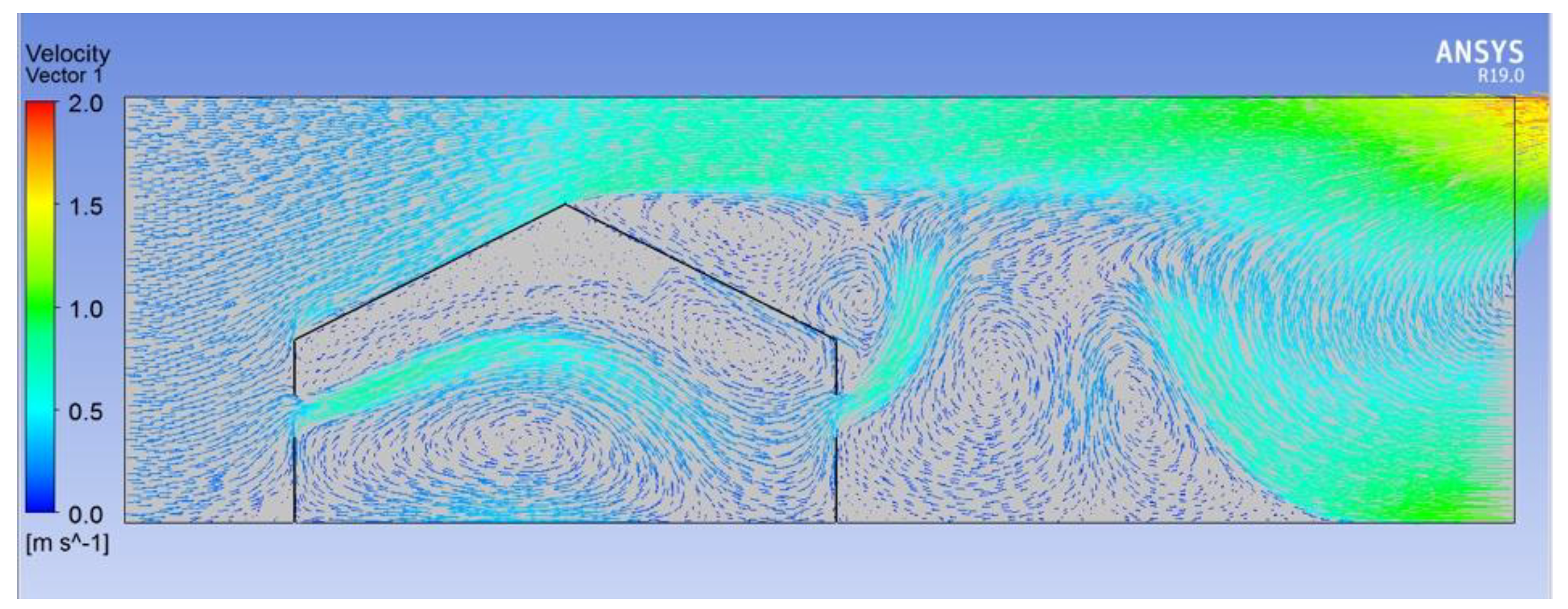
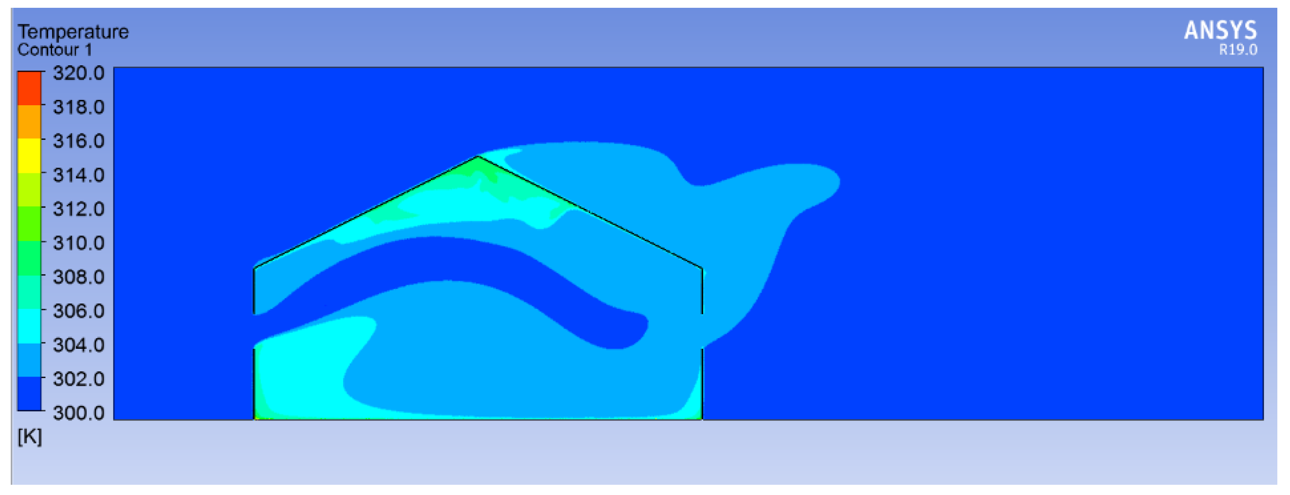
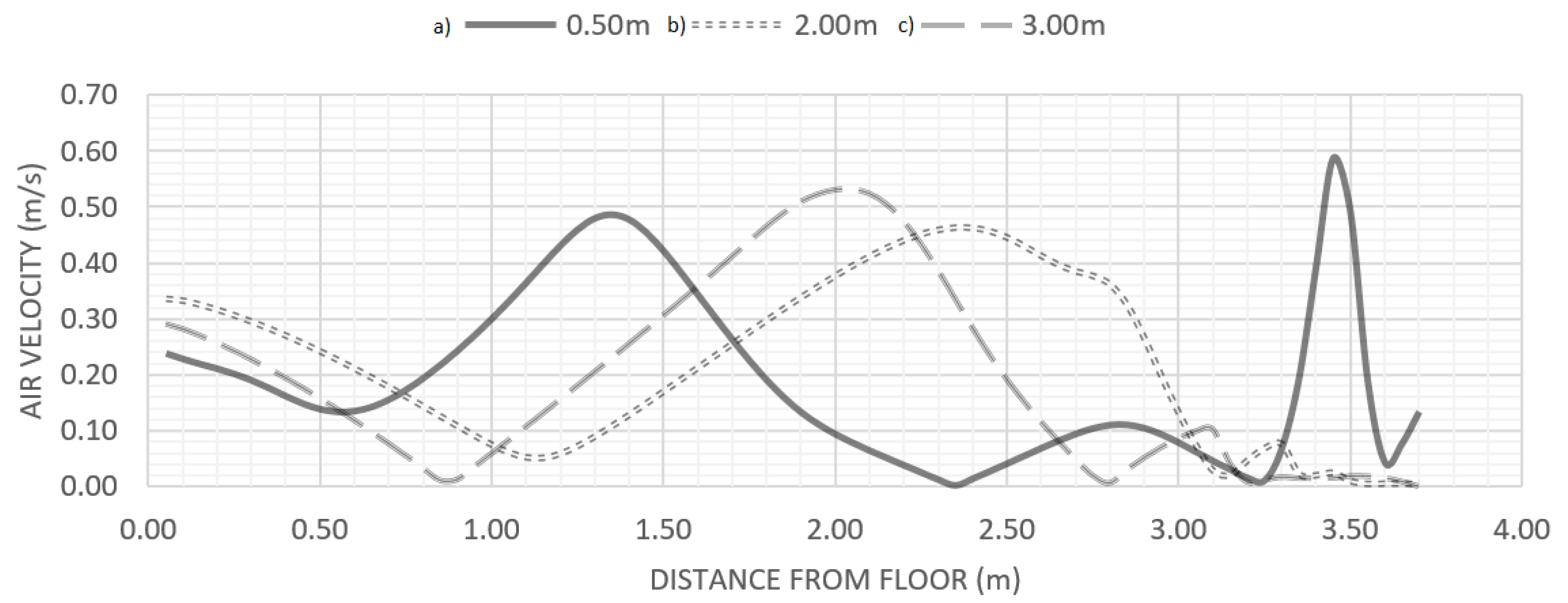
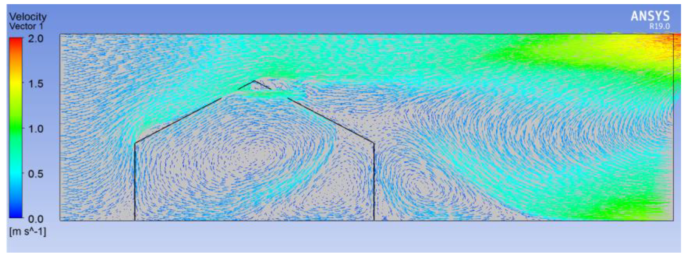
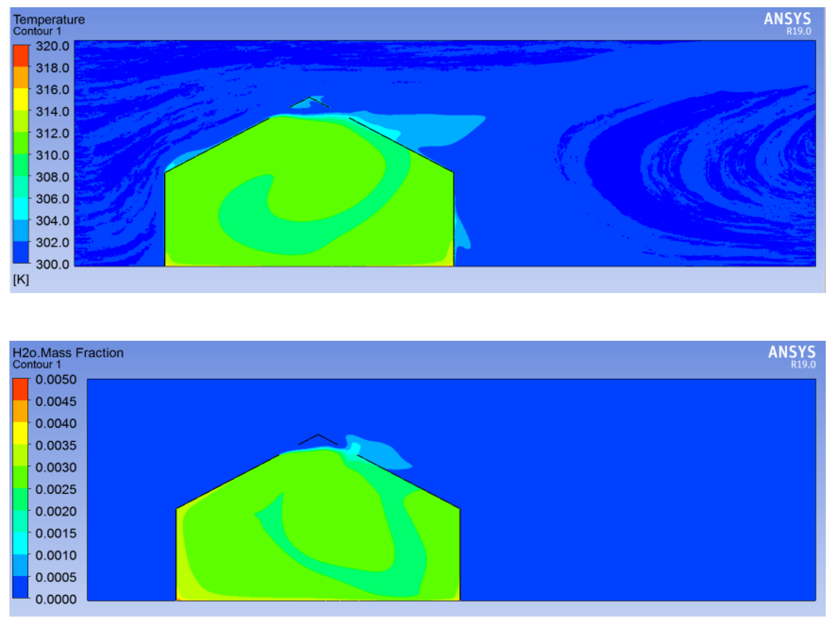
4.1. Results of the Side Vent Analysis

The results from the side vent geometry analysis show that for low wind speeds, the height of the vent influences the air-flow pattern inside the GH. When the vent is towards the floor of the GH, there is a fast-moving air current along the floor of the GH, as seen in Figure 6. This air causes a counter-clockwise rotating air loop to form above the air current, which fills almost all of the GH. As the side vent moves towards the centre of the wall, like in the initial model (see Figure 3), the counter-clockwise loop decreases in size, and a clockwise loop of air forms below the air entering the GH. When the side vents are at the top of the wall, the counter-clockwise loop no longer exists, and the air enters the windward side vent, follows the roof upwards to the ridge, then flows back down the leeward roof, where some air exits the leeward side vent and most of the air goes towards the floor and back to the windward wall, creating a large clockwise circular air-flow pattern (see Figure 7).
The dominance of the buoyancy effect is demonstrated by the air-flow patterns, as when air along the floor in every simulation is heated, it rises upwards instead of flowing along the floor. The buoyancy effect is the driving force behind the circular air-flows, as when the inlet flows are along the floor, the air rises up and forms a counter-clockwise circular flow, whereas when the vents are at the top of the wall, the stagnant air below the vent is heated and rises up into the inlet air-flow, which causes the clockwise flow of air around the GH.
The position of the side vents also affects the temperature distribution inside the GH, as in every model, the air below the vent has a higher temperature than that of the air entering the GH. For this model, using a vent position at the top of the wall causes temperatures in some locations to increase by 2 K to 4 K when compared to a vent positioned at the bottom of the wall. The temperature contours for a high and low side vent position are displayed in Figure 3 and Figure 4 and show that the temperature of the air in the GH for the horizontal distance from the windward vent, at a height of 1m for a low (0.25 m), central (1 m) and high (1.5 m) side vent position, and the temperature at plant level for the high side vent GH is at least 2 K higher than the temperature of the low side vent for every distance, whilst the temperature for the central side vent design is dependent on the distance from the vent, as the air current from the windward vent affects the temperature at this height. It should also be noted that while the low side vent provides better cooling, it has a higher velocity of air-flow at the plant level, as shown in Figure 6, which may cause damage to plants.
The water vapour mass fraction contour follows a similar pattern to that of the temperature contour. For low vent positions, the water vapour does not rise very far above the floor before it is taken by the air current from the windward side vent, and exits the leeward side vent, as shown in Figure 6. For higher side vents, the water vapour is taken by the air into the clockwise circling air pattern, and so the humidity in the air increases before exiting the leeward side vent, as seen in Figure 7. This also suggests that the ventilation rate is less efficient for higher side vent positions.

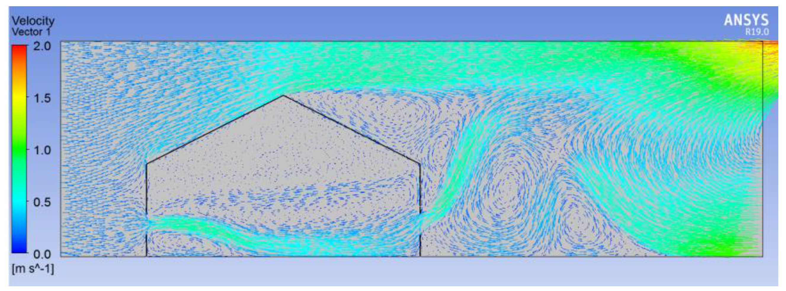
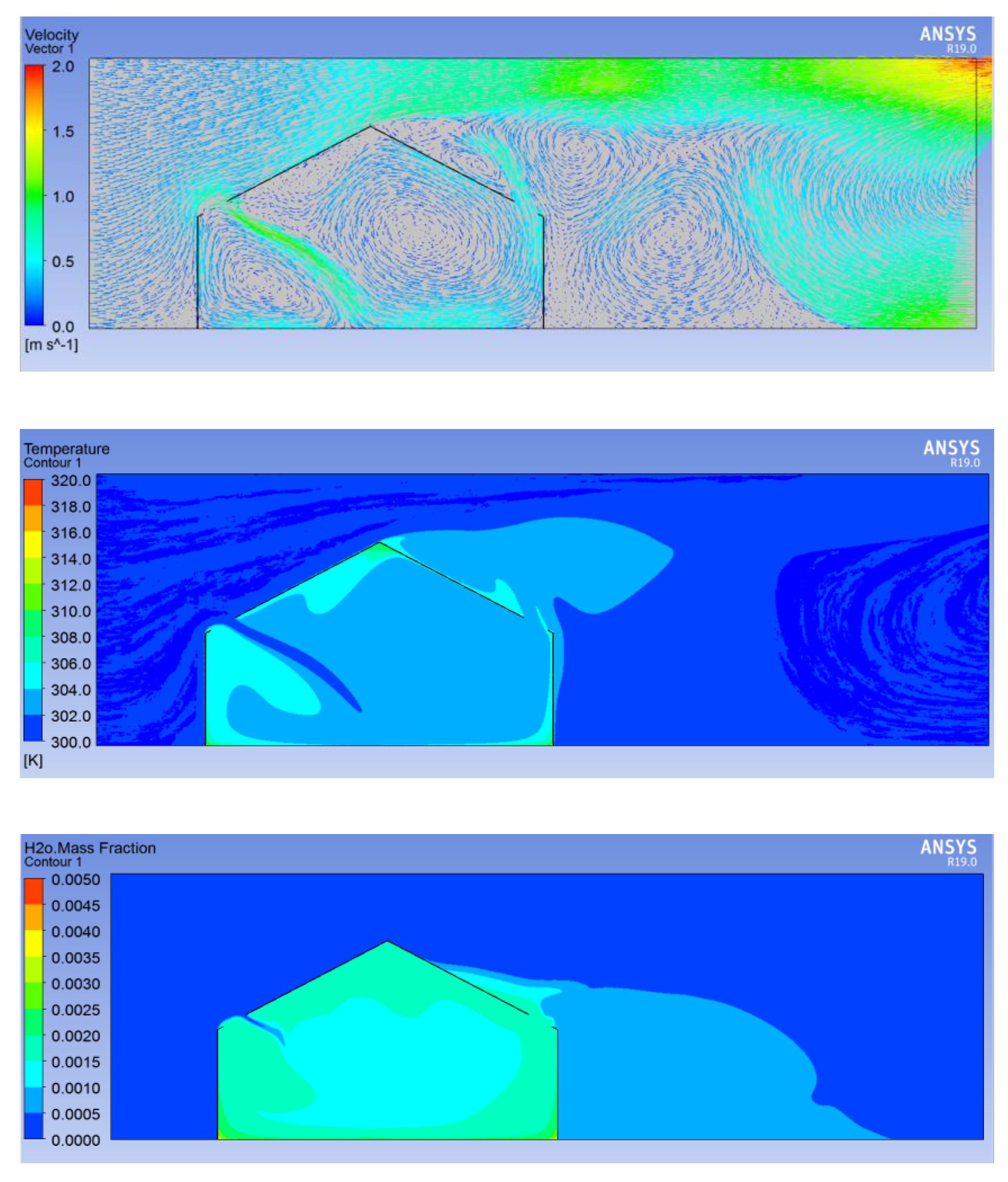
4.2. Results of the Roof Vent Analysis

The position of the roof vents does not have as great an impact on the variables studied as the position of the side vents. As the distance of the roof vent from the ridge increases, the clockwise circular air-flow pattern formed in the initial model increases in size to fill more of the GH. A larger percentage of the air from the roof vent joins the air current from the side vent, making the current larger and increasing the velocity of the air. Additionally, the fast-moving air tends to be at the same height as the roof vent, which means that for the low roof vents, such as in Figure 8, there is very little air movement in the roof of the GH.
The temperature contours are like that of the initial model, particularly at the plant level where the temperature increases by between 2 K and 6 K in all simulations, compared with the external air temperature. The effect of the roof vents on the temperature, as was with the air velocity, is that the temperature in the roof of the GH increases by up to 10 K as the roof vents are placed further away from the GH ridge, as seen in Figure 8. However, this is a small area, so the temperature increase would have a minimal effect on the conditions of the GH at the plant level.
The position of the roof vent has no effect on the water vapour contour, with every result being virtually identical to the initial model, as seen in Figure 3.

4.3. Results of Side Vent Analysis without Roof Vents

The air-flow pattern formed when the roof vents are removed, as seen in Figure 3, is still very similar to the air-flow in the initial model, which is shown in Figure 3. The air enters through the windward side vent of the GH and creates the same clockwise air loop below the vent. The difference between the original model is in the outflow of the air, as Figure 3 shows that in the initial model, most of the air exits the GH through the leeward roof vent. However, as Figure 9 shows, there is no roof vent in the model, so most of the air instead exits through the leeward side vent. This causes poor air renewal rate in the roof of the GH.
This is also shown in Figure 10, which plots the air velocities for the vertical height above the floor at the centre of the GH, for a roof vent placed close to the ridge (0.5 m), in the centre of the roof (2 m) and far away from the ridge (3 m). It shows that for the vent placed close to the ridge, the air velocity has two peaks, due to the two separate air currents developed in the initial model (Figure 3), and as the vent moves further from the ridge of the GH, the maximum velocity of the air occurs closer to the floor of the GH. It also shows that there is very little air movement above the air current caused by the roof vents. This can also be seen in Figure 7 where the temperature is analysed against the vertical height above the floor at the centre of the GH, for the initial model and the models without side vents. The position of the side vents is also analysed when the roof vents are removed, and for the high side vent design, the air-flow pattern is very similar.
This shows that the roof vent has very little effect on the air-flow for the high side vents as the clockwise circular air pattern still forms. However, for the low side vent position, the air enters the windward side vent, travels along the floor and out the leeward side vent, so the counter-clockwise air loop does not form, and there is very little air movement in the roof of the GH, as seen in Figure 11.
When the roof vents are further from the ridge (Figure 8) the temperature increases in the roof of the GH when the roof vents are removed, as the warm air is not efficiently ventilated. This means that the temperature in the roof increases by up to 6 K for the low side vent model, seen in Figure 11, when compared to the same GH design with roof vents included in the standard position, as in the initial model. However, as the high side vent design maintains the same clockwise air pattern without roof vents, the average temperature in this design is much lower, maintaining the same temperatures. The initial model shows a much lower temperature than the same model without the roof vent, particularly in the roof, as the temperature is 7 K higher for the closed roof vent model with the side vent in the same position as the original model. The high side vent position maintains the same air-flow pattern without the roof vent, which causes much more effective cooling than the other models analysed since the temperature stays at about 304 K until it reaches the very top of the roof. As with other results, the water vapour stays below the windward vent, where it builds up in the slower-moving air and where the temperature is also higher. Most of the water vapour is found below the windward vent, as the stronger air current flows over the corner and develops the rotating flow patterns. The water vapour is naturally removed by the air current and exits through the leeward side vent.

4.4. Results of the Roof Vent Analysis without Side Vents

The effect of the side vents on the ventilation of the GH is clearly seen by comparing Figure 12 with Figure 3. The air-flow pattern is different, and the average velocity of the air in the GH is lower, which causes a temperature increase of around 9K, and also causes the water vapour mass fraction to greatly increase. This temperature difference (see Figure 13) suggests that the ventilation rate is much lower, which is expected, as the side vents account for most of the air-flow into the GH in the initial model.
The effect of the position of the roof vent can also be studied. In the original roof vent position when the GH has no side vents, the air enters the windward roof vent and forms a clockwise circle of air that fills most of the GH, and some of the air forms a smaller, counter-clockwise circular air pattern by the leeward wall, as seen in Figure 12.
As the vent position moves away from the ridge of the GH, the counter-clockwise rotating air dissolves, and the clockwise loop fills the GH. When the vent is just above the wall, as far from the ridge as possible, the direction of the air-flow changes, as shown in Figure 14. Instead of moving along the roof and down the leeward wall, a fast-moving current of air moves directly from the windward vent to the centre of the floor and forms a counter-clockwise pattern by moving up the leeward wall, with some air exiting the leeward vent and the rest moving up the leeward roof to complete the circular flow. A smaller clockwise circular air-flow also forms from the air moving to the left once it reaches the floor.
The temperature contours show that the designs where the roof vents are further from the ridge are much more efficient at cooling the GH and maintaining a temperature closer to that of the outside temperature, which can be seen by comparing Figure 8 and Figure 9. The most likely cause of this is that as the vents are moved further apart, a lower percentage of the air that enters the GH can exit directly through the leeward vent, so the air renewal is more efficient, and the temperature is lower. The cold air-flow seen from the windward vent on Figure 14 is the fast-moving air described previously, which has a significant effect on the temperature of the rest of the GH. Comparing the temperature profile with the air-flow pattern for both Figure 8 and Figure 9 shows the effect of the flow on the temperature of the air, as both figures show that where the cooler external air enters the GH at relatively high velocities, the temperature contours show a lower temperature in that area.
The temperatures in the GH at different heights above the floor are compared in Figure 13, for the initial model; and for the model with a roof vent placed close to the ridge (0.5 m), slightly further from the ridge (1 m), in the centre of the roof (2 m), and far from the ridge (3 m); each without a side vent. The effect of the side vent can be seen by comparing the initial model with the same roof vent position (0.5 m) and no side vent, as the model without the side vent is between 6 K and 9 K higher for much of the GH. This also shows that the temperature decreases as the roof vent moves further away from the ridge, for the models with no side vents, as the model with roof vents furthest away from the ridge has a temperature distribution very similar to that of the initial model.
The pattern of the water vapour mass fraction contour is very similar for the different models analysed. The contours tend to the air-flow patterns, as the water vapour builds up in areas where the air velocity is lower, so the air renewal rate is also lower. The model shown in Figure 14 has a lower temperature than the model with the roof vents 2 m from the ridge but has a higher water vapour contour for the different air-flow patterns described above. This suggests that if the air can stagnate above the roof vents, as it does in Figure 14, then the percentage of water vapour in the air can increase, even though the temperature of the air is lower. This would increase the GH humidity level.

4.5. Results of the Sensitivity of the Wind Speed

The external wind speed does not have much effect on the air-flow patterns in the GH for this model, which is apparent when comparing Figure 15 with Figure 3. The air-flow is generally the same pattern as described in the initial model. This is expected to be the case, as for all the external wind speeds analysed, the buoyancy effect should still be the driving force, so changing the wind speed would have little impact on the air-flow distribution. However, the air velocity does increase as the external wind increases. The air velocity at the windward vent given as a ratio of the external wind speed was analysed in Figure 4 for the four simulations studied. Figure 16 shows the ratio decreasing until it reaches the value of one, as the external wind speed would increase until it is the dominant effect, at which point pressure differences caused by the buoyancy effect should have a negligible effect on the average wind velocity through the side vent, thus producing a wind velocity through the side vent that is equal to the external wind velocity. However, not enough analysis of higher wind speeds was performed to state with certainty that this is the case.
The temperature contours were also very similar to the original model. This also proves that the wind speed has very little effect on the ventilation of the GH at low wind speeds, when the buoyancy effect drives the ventilation mechanism. The water vapour level gradually decreases as the wind speed increases, the most likely cause of which is that the higher wind speeds can more efficiently ventilate the areas of the GH where the air is slower-moving. This causes the air renewal rate to increase in these areas, thus meaning less water vapour per unit volume of air.

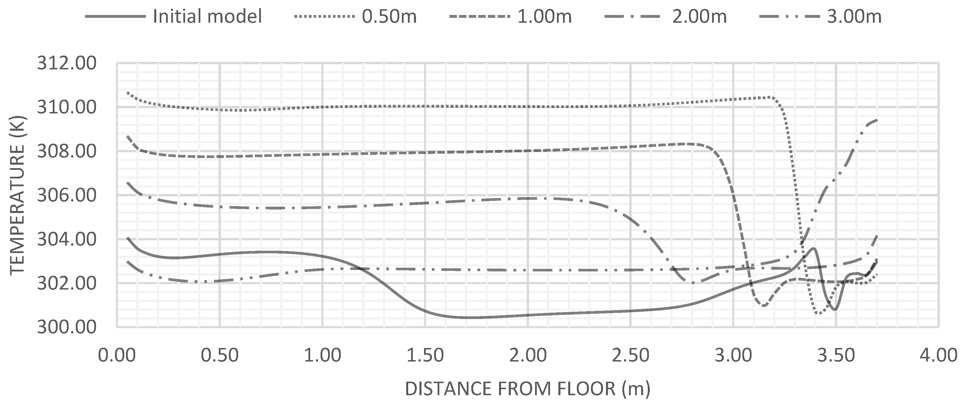
4.6. Results of the Sensitivity of the Floor Heating Analysis

The analysis of the floor temperature on the air velocity and pattern showed that there was very little effect on either variable. The air-flow patterns that formed were almost identical to those of the initial model, as seen in Figure 3. This is likely due to the small changes in temperature that occur in the GH, which would not have much of an effect on the buoyancy forces acting on the air molecules.
The temperature and humidity contours are also qualitatively very similar in each of the models, for the same reasons as given above. However, the temperature does quantitatively increase with the increase in floor temperature. Figure 17 compares the temperatures at the vertical displacements above the floor, for the models with floor temperatures of 310 K, 315 K, 320 K and 325 K. The temperatures vary slightly for most of the GH, as increasing the floor temperature by 5 K increases the average temperature by around 1 K. However, Figure 18 shows that the temperature distributions around the GH are the same.

5. Conclusions

The initial 2D model designed in this study was validated by the work performed experimentally by Sase et al. [35] and using CFD methods by Mistrotis et al. [20]. The air-flow pattern and temperature contour were both found to be quantitatively very similar to both studies mentioned. Additionally, the humidity was found to be highest under the windward vent, where the air renewal rate was lower than in the rest of the GH. The initial 3D model showed a very similar flow pattern to the 2D model, where most studies found that for a wind direction perpendicular to the GH ridge, the variables were almost independent of the GH end walls. The humidity was also found to be higher in the same place than it was in the 2D model.
The geometrical analysis found that the position of the side vents caused a reversal of the direction of the air loop formed in the GH and found that the temperature was higher at the crop level when the side vents were located higher up the wall of the GH. The humidity was also found to increase with higher side vent positions. A similar conclusion was made by Bournet et al. [39,67] for multi-span GHs, which was that the high side vent provided a lower air renewal rate and greater heterogeneity of temperature at the plant level. The importance of the side vent was also analysed, as temperatures in the GH could increase by almost 10 K if no side vent was designed. The humidity was also much higher in the GHs with no side vents.
The roof vent position was found to have less of an effect on the ventilation, air-flow pattern and temperature at the plant level. However, it was shown to have a much greater effect on the ventilation in the roof, as the air became stagnant above the height of the roof vent, causing higher temperatures. The same conclusion was also made when the roof vents were removed, as the temperatures increased rapidly in the roof. The position of the roof vent had no effect on the humidity. When the side vents were removed, the roof vent position was more influential, as the average temperature decreased when the roof vent was moved further from the ridge.
The external wind speed was shown to have very little effect on the air-flow pattern, temperature and humidity for the wind speeds studied, as the buoyancy effect was the driving ventilation force in all simulations tested. The temperature was shown to increase with increased floor temperature, but this also had no impact on either the air-flow pattern or humidity.
Therefore, for the MENA countries, several side vents should be designed to open in different combinations when the temperature or the relative humidity reaches a certain amount or for different environmental conditions. The area which hosted the plants could be designed as a cavity to preserve their microclimate conditions, while the extra humidity could get condensed using dehumidification techniques. For the countries having hot climate conditions, one or multiple roof vents should be designed to release the extra heat for the intense conditions, when necessary.

Author Contributions

Conceptualisation, M.A., M.J.H., A.A.J., and A.N.; Methodology, M.A. and M.J.H.; Software, M.A. and A.A.J.; Validation, M.A., M.J.H., and M.D.; Investigation, A.A.J., R.F., and A.N.; Writing—original draft prepapartion, M.A., M.J.H., M.D., A.A.J., G.R.T.; Writing—review and editing, M.A., A.A.J., G.R.T., M.D. All authors have read and agreed to the published version of the manuscript.

Funding

This work was supported by the British Council (BC) of UK (No. 332435306) and Science & Technology Development Fund (STDF) of Egypt (No. 30771), through the project titled “A Novel Standalone Solar-Driven Agriculture Greenhouse-Desalination System: That Grows its Energy and Irrigation Water” via the Newton-Musharafa funding scheme.

Acknowledgments

The authors would like to acknowledge Anthony Cockell, Iain Park and Vikki Price for their support during the data collection from the greenhouse. The authors would like to appreciate the anonymous reviewers for their insightful comments and suggestions.

Conflicts of Interest

The authors declare no conflict of interest.

Nomenclature

Acronyms
CFDComputational Fluid Dynamics
CO2Carbon Dioxide
GHGreenhouse
MENAMiddle East and North Africa
Symbols
ΔP(y)Vertical profile of Pressure drop
v(y)Vertical profile of air velocity
ρAir density
ζPressure drop coefficient
A1Discharge coefficient
GVolumetric flow rate
LLength of vent
HHeight of vent
gGravity constant
TTemperature
SEffective opening area of vents
μ t Eddy viscosity
σ k , σ ϵ Turbulent Prandtl numbers (constant)
G k Generation of k due to mean velocity gradients
G b Generation of k due to buoyancy
Y M Contribution of fluctuating dilation in compressible turbulence to overall dissipation rate
S k , S ϵ User-defined source terms
C 1 ϵ , C 2 ϵ , C 3 ϵ Model constants
k e f f Effective conductivity
h j Sensible enthalpy
J j Diffusion flux for species j
τ = e f f Effective stress tensor
S h User-defined heat sources
Y i Local mass fraction of species j
R i Rate of production of species by chemical reaction
S i Rate of creation by addition from dispersed phase and user-defined sources
D i , m Mass diffusion coefficient for species
S c t Schmidt number
D T , i Turbulent diffusion coefficient

References

  1. Fath, H.E.-B.S. Desalination and Greenhouses. In The Handbook of Environmental Chemistry; Springer: Cham, Switzerland, 2017; Volume 75, pp. 455–483. [Google Scholar]
  2. Fath, H.E.; Javadi, A.A.; Akrami, M.; Farmani, R.; Negm, A.; Mallick, T. A Novel stand-alone solar-powered agriculture greenhouse-desalination system; increasing sustainability and efficiency of greenhouses. In Proceedings of the Innovative Applied Energy (IAPE) Conference, Oxford, UK, 14–15 March 2019. [Google Scholar]
  3. Panahi, R.; Khanjanpour, M.H.; Javadi, A.A.; Akrami, M.; Rahnama, M.; Ameri, M. Analysis of the thermal efficiency of a compound parabolic Integrated Collector Storage solar water heater in Kerman, Iran. Sustain. Energy Technol. Assess. 2019, 36, 100564. [Google Scholar] [CrossRef]
  4. Alotaibi, D.M.; Akrami, M.; Dibaj, M.; Javadi, A.A. Smart energy solution for an optimised sustainable hospital in the green city of NEOM. Sustain. Energy Technol. Assess. 2019, 35, 32–40. [Google Scholar] [CrossRef]
  5. Alnaser, W.; Trieb, F.; Knies, G. Solar energy technology in the Middle East and North Africa (MENA) for sustainable energy, water and environment. Adv. Solar Energy 2007, 17, 261. [Google Scholar]
  6. El-Ghonemy, A. RETRACTED: Future sustainable water desalination technologies for the Saudi Arabia: A review. Renew. Sustain. Energy Rev. 2012, 16, 6566–6597. [Google Scholar] [CrossRef]
  7. Mahmoud, A.; Fath, H.; Ahmed, M. Enhancing the performance of a solar driven hybrid solar still/humidification-dehumidification desalination system integrated with solar concentrator and photovoltaic panels. Desalination 2018, 430, 165–179. [Google Scholar] [CrossRef]
  8. Ghaffour, N. The challenge of capacity-building strategies and perspectives for desalination for sustainable water use in MENA. Desalin. Water Treat. 2009, 5, 48–53. [Google Scholar] [CrossRef]
  9. Negm, A.M.; Omran, E.-S.E.; Mahmoud, M.A.; Abdel-Fattah, S. Update, Conclusions, and Recommendations for Conventional Water Resources and Agriculture in Egypt. In Unconventional Water Resources and Agriculture in Egypt, The Handbook of Environmental Chemistry; Springer: Cham, Switzerland, 2018; Volume Voulme 75, pp. 659–681. [Google Scholar] [CrossRef]
  10. Kittas, C.; Draoui, B.; Boulard, T. Quantification of the ventilation of a greenhouse with a roof opening. Agric. For. Meteorol. 1995, 1, 95–111. [Google Scholar] [CrossRef]
  11. Kittas, C.; Boulard, T.; Mermier, M.; Papadakis, G. Wind Induced Air Exchange Rates in a Greenhouse Tunnel with Continuous Side Openings. J. Agric. Eng. Res. 1996, 65, 37–49. [Google Scholar] [CrossRef]
  12. Baptista, F.; Bailey, B.; Randall, J.; Meneses, J. Greenhouse Ventilation Rate: Theory and Measurement with Tracer Gas Techniques. J. Agric. Eng. Res. 1999, 72, 363–374. [Google Scholar] [CrossRef] [Green Version]
  13. Kacira, M.; Sase, S.; Ikeguchi, A.; Ishii, M.; Giacomelli, G.; Sabeh, N. Effect of vent configuration and wind speed on three-dimensional temperature distributions in a naturally ventilated multi-span greenhouse by wind tunnel experiments. Acta Hortic. 2008, 801, 393–401. [Google Scholar] [CrossRef]
  14. Bartzanas, T.; Boulard, T.; Kittas, C. Effect of Vent Arrangement on Windward Ventilation of a Tunnel Greenhouse. Biosyst. Eng. 2004, 88, 479–490. [Google Scholar] [CrossRef]
  15. Bartzanas, T.; Kittas, C.; Sapounas, A.; Nikita-Martzopoulou, C. Analysis of airflow through experimental rural buildings: Sensitivity to turbulence models. Biosyst. Eng. 2007, 97, 229–239. [Google Scholar] [CrossRef]
  16. Norton, T.; Sun, D.-W.; Grant, J.; Fallon, R.; Dodd, V. Applications of computational fluid dynamics (CFD) in the modelling and design of ventilation systems in the agricultural industry: A review. Bioresour. Technol. 2007, 98, 2386–2414. [Google Scholar] [CrossRef] [PubMed]
  17. Lee, I.-B.; Short, T.H. Two-dimensional numerical simulation of natural ventilation in a multi-span greenhouse. Trans. ASAE 2000, 43, 745–753. [Google Scholar] [CrossRef]
  18. Wang, S.; Boulard, T. Measurement and prediction of solar radiation distribution in full-scale greenhouse tunnels. Agronomie 2000, 20, 41–50. [Google Scholar] [CrossRef]
  19. Shklyar, A.; Arbel, A. Numerical model of the three-dimensional isothermal flow patterns and mass fluxes in a pitched-roof greenhouse. J. Wind. Eng. Ind. Aerodyn. 2004, 92, 1039–1059. [Google Scholar] [CrossRef]
  20. Mistriotis, A.; Arcidiacono, C.; Picuno, P.; Bot, G.; Scarascia-Mugnozza, G. Computational analysis of ventilation in greenhouses at zero- and low-wind-speeds. Agric. For. Meteorol. 1997, 88, 121–135. [Google Scholar] [CrossRef]
  21. Nebbali, R.; Roy, J.; Boulard, T.; Makhlouf, S. Comparison of the accuracy of different cfd turbulence models for the prediction of the climatic parameters in a tunnel greenhouse. Acta Hortic. 2006, 287–294. [Google Scholar] [CrossRef]
  22. Roy, J.; Boulard, T. CFD prediction of the natural ventilation in a tunnel-type greenhouse: Influence of wind direction and sensibility to turbulence models. In International Conference on Sustainable Greenhouse Systems-Greensys 2004, Proceedings of the Greensys 2004, Leuven, Belgium, September 2004; International Society for Horticultural Science: Leauven, Belgium, 2005. [Google Scholar]
  23. Baeza, E.J.; Pérez-Parra, J.J.; Montero, J.I.; Bailey, B.J.; López, J.C.; Gázquez, J.C. Analysis of the role of sidewall vents on buoyancy-driven natural ventilation in parral-type greenhouses with and without insect screens using computational fluid dynamics. Biosyst. Eng. 2009, 104, 86–96. [Google Scholar] [CrossRef]
  24. Kacira, M.; Short, T.H.; Stowell, R.R. A cfd evaluation of naturally ventilated, multi-span, sawtooth greenhouses. Trans. ASAE 1998, 41, 833–836. [Google Scholar] [CrossRef]
  25. Fatnassi, H.; Boulard, T.; Demrati, H.; Bouirden, L.; Sappe, G. SE—Structures and Environment: Ventilation Performance of a Large Canarian-Type Greenhouse Equipped with Insect-Proof Nets. Biosys. Eng. 2002, 82, 97–105. [Google Scholar] [CrossRef]
  26. Montero, J.; Muñoz, P.; Antón, A.; Iglesias, N. Computational fluid dynamic modelling of night-time energy fluxes in unheated greenhouses. Acta Hortic. 2005, 691, 403–410. [Google Scholar] [CrossRef]
  27. Bournet, P.E.; Winiarek, V.; Chasseriaux, G. Coupled energy radiation balance in a closed partitioned glass house during night using computational fluid dynamics. In Proceedings of the International Symposium on Greenhouse Cooling: Methods, Technologies and Plant Response, Alméria, Spain, 24–27 April 2006. [Google Scholar]
  28. Both, A.; Reiss, E.; Mears, D.; Roberts, W. Open-roof Greenhouse Design with Heated Ebb and Flood Floor. In Proceedings of the 2001 ASAE Annual Meeting, Sacramento, CA, USA, 29 July–1 August 2001. [Google Scholar]
  29. Sase, S.; Reiss, E.; Both, A.; Roberts, W. A Natural Ventilation Model for Open-Roof Greenhouses. In Proceedings of the 2002 ASAE Annual Meeting, Chicago, IL, USA, 28–31 July 2002. [Google Scholar]
  30. Bony, S.; Lau, K.-M.; Sud, Y.C. Sea Surface Temperature and Large-Scale Circulation Influences on Tropical Greenhouse Effect and Cloud Radiative Forcing. J. Clim. 1997, 10, 2055–2077. [Google Scholar] [CrossRef]
  31. Patil, S.; Tantau, H.; Salokhe, V. Modelling of tropical greenhouse temperature by auto regressive and neural network models. Biosyst. Eng. 2008, 99, 423–431. [Google Scholar] [CrossRef]
  32. Lamrani, M.A.; Boulard, T.; Roy, J.C.; Jaffrin, A. Airflow and temperature patterns induced in a confined greenhouse. J. Agric. Eng. Res. 2001, 78, 75–88. [Google Scholar] [CrossRef]
  33. Boulard, T.; Haxaire, R.; Lamrani, M.; Roy, J.; Jaffrin, A. Characterization and Modelling of the Air Fluxes induced by Natural Ventilation in a Greenhouse. J. Agric. Eng. Res. 1999, 74, 135–144. [Google Scholar] [CrossRef]
  34. Papadakis, G.; Mermier, M.; Meneses, J.; Boulard, T. Measurement and Analysis of Air Exchange Rates in a Greenhouse with Continuous Roof and Side Openings. J. Agric. Eng. Res. 1996, 63, 219–228. [Google Scholar] [CrossRef]
  35. Sase, S.; Takakura, T.; Nara, M. Wind tunnel testing on airflow and temperature distribution of a naturally ventilated greenhouse. Acta Hortic. 1984, 148, 329–336. [Google Scholar] [CrossRef]
  36. Bournet, P.-E.; Boulard, T. Effect of ventilator configuration on the distributed climate of greenhouses: A review of experimental and CFD studies. Comput. Electron. Agric. 2010, 74, 195–217. [Google Scholar] [CrossRef]
  37. Salah, A.H.; Hassan, G.E.; Fath, H.; Elhelw, M.; Elsherbiny, S. Analytical investigation of different operational scenarios of a novel greenhouse combined with solar stills. Appl. Therm. Eng. 2017, 122, 297–310. [Google Scholar] [CrossRef]
  38. Kabir Abdullahi, M.; Salah, A.H.; Fath, H.E. Micro Climatic Analysis of Sustainable Agricultural Greenhouse with Built-In Roof Solar Stills. In Proceedings of the Innovative Applied Energy (IAPE) Conference, Oxford, UK, 14–15 March 2019. [Google Scholar]
  39. Bournet, P.E.; Khaoua, S.A.O.; Boulard, T.; Migeon, C.; Chasseriaux, G. Effect of Roof and Side Opening Combinations on the Ventilation of a Greenhouse Using Computer Simulation. Trans. ASABE 2007, 50, 201–212. [Google Scholar] [CrossRef]
  40. Kim, K.; Yoon, J.-Y.; Kwon, H.-J.; Han, J.-H.; Son, J.E.; Nam, S.-W.; Giacomelli, G.A.; Lee, I.-B. 3-D CFD analysis of relative humidity distribution in greenhouse with a fog cooling system and refrigerative dehumidifiers. Biosyst. Eng. 2008, 100, 245–255. [Google Scholar] [CrossRef]
  41. Benni, S.; Tassinari, P.; Bonora, F.; Barbaresi, A.; Torreggiani, D. Efficacy of greenhouse natural ventilation: Environmental monitoring and CFD simulations of a study case. Energy Build. 2016, 125, 276–286. [Google Scholar] [CrossRef]
  42. Arbel, A.; Barak, M.; Shklyar, A. Combination of Forced Ventilation and Fogging Systems for Cooling Greenhouses. Biosyst. Eng. 2003, 84, 45–55. [Google Scholar] [CrossRef]
  43. Campen, J.; Bot, G. Determination of Greenhouse-specific Aspects of Ventilation using Three-dimensional Computational Fluid Dynamics. Biosyst. Eng. 2003, 84, 69–77. [Google Scholar] [CrossRef]
  44. Boulard, T.; Baille, A. Modelling of Air Exchange Rate in a Greenhouse Equipped with Continuous Roof Vents. J. Agric. Eng. Res. 1995, 61, 37–47. [Google Scholar] [CrossRef]
  45. Spiegel, E.A.; Veronis, G. On the Boussinesq Approximation for a Compressible Fluid. Astrophys. J. 1960, 131, 442. [Google Scholar] [CrossRef]
  46. ANSYS FLUENT 12-Theory Guide, ANSYS FLUENT. Available online: https://www.afs.enea.it/project/neptunius/docs/fluent/html/th/main_pre.htm (accessed on 1 December 2019).
  47. Yates, M.; Akrami, M.; Javadi, A.A. Analysing the performance of liquid cooling designs in cylindrical lithium-ion batteries. J. Energy Storage 2019, 100913. [Google Scholar] [CrossRef]
  48. Bandmann, C.E.; Akrami, M.; Javadi, A.A. An investigation into the thermal comfort of a conceptual helmet model using finite element analysis and 3D computational fluid dynamics. Int. J. Ind. Ergon. 2018, 68, 125–136. [Google Scholar] [CrossRef]
  49. Gebreslassie, M.G.; Tabor, G.R.; Belmont, M.R. Investigation of the performance of a staggered configuration of tidal turbines using CFD. Renew. Energy 2015, 80, 690–698. [Google Scholar] [CrossRef] [Green Version]
  50. Tabor, G.; Jarman, D.; Andoh, R.; Butler, D.; Galambos, I.; Djordjevic, S. Application of Open Source CFD in Urban Water Management. In World Environmental and Water Resources Congress 2011: Bearing Knowledge for Sustainability, Proceedings of the World Environmental and Water Resources Congress 2011: Bearing Knowledge for Sustainability 2011, Palm Springs, CA, USA, 22–26 May 2011; American Society of Civil Engineers: Reston, VA, USA, 2011. [Google Scholar]
  51. Arfaei, A.; Hançer, P. Effect of the Built Environment on Natural Ventilation in a Historical Environment: Case of the Walled City of Famagusta. Sustainability 2019, 11, 6043. [Google Scholar] [CrossRef] [Green Version]
  52. Liu, J.; Heidarinejad, M.; Nikkho, S.K.; Mattise, N.W.; Srebric, J. Quantifying Impacts of Urban Microclimate on a Building Energy Consumption—A Case Study. Sustainability 2019, 11, 4921. [Google Scholar] [CrossRef] [Green Version]
  53. Bustamante, E.; García-Diego, F.-J.; Calvet, S.; Torres, A.G.; Hospitaler, A. Measurement and Numerical Simulation of Air Velocity in a Tunnel-Ventilated Broiler House. Sustainability 2015, 7, 2066–2085. [Google Scholar] [CrossRef] [Green Version]
  54. He, X.; Wang, J.; Guo, S.; Zhang, J.; Wei, B.; Sun, J.; Shu, S. Ventilation optimization of solar greenhouse with removable back walls based on CFD. Comput. Electron. Agric. 2018, 149, 16–25. [Google Scholar] [CrossRef]
  55. Villagrán, E.A.; Romero, E.J.B.; Bojacá, C.R. Transient CFD analysis of the natural ventilation of three types of greenhouses used for agricultural production in a tropical mountain climate. Biosyst. Eng. 2019, 188, 288–304. [Google Scholar] [CrossRef]
  56. Cao, L.Y.; Wu, J.H.; Hu, Y.; Gu, X.B.; Liu, W.W.; Cao, H.Z. Cooling Effect of Mechanical Ventilation in Grape Greenhouse Based on CFD Numerical Simulation. Appl. Mech. Mater. 2014, 448, 2890–2896. [Google Scholar] [CrossRef]
  57. Santolini, E.; Pulvirenti, B.; Benni, S.; Barbaresi, L.; Torreggiani, D.; Tassinari, P. Numerical study of wind-driven natural ventilation in a greenhouse with screens. Comput. Electron. Agric. 2018, 149, 41–53. [Google Scholar] [CrossRef]
  58. Cemek, B.; Atiş, A.; Küçüktopçu, E. Evaluation of temperature distribution in different greenhouse models using computational fluid dynamics (CFD). Anadolu J. Agric. Sci. 2017, 32, 54. [Google Scholar] [CrossRef] [Green Version]
  59. Aich, W.; Kolsi, L.; Borjini, M.N.; Aissia, H.B.; Öztop, H.; Abu-Hamdeh, N. Three-dimensional CFD Analysis of Buoyancy-driven Natural Ventilation and Entropy Generation in a Prismatic Greenhouse. Therm. Sci. 2016, 52. [Google Scholar] [CrossRef]
  60. Okushima, L.; Sase, S.; Nara, M. A support system for natural ventilation design of greenhouses based on computational aerodynamics. Acta Hortic. 1989, 248, 129–136. [Google Scholar] [CrossRef]
  61. Mohammadi, B.; Pironneau, O. Analysis of the k-ϵ Turbulence Model. In Research in Applied Mathematics; Wiley-Masson: Paris, France, 1994. [Google Scholar]
  62. Hu, J.; Cai, W.; Li, C.; Gan, Y.; Chen, L. In situ x-ray diffraction study of the thermal expansion of silver nanoparticles in ambient air and vacuum. Appl. Phys. Lett. 2005, 86, 151915. [Google Scholar] [CrossRef]
  63. Tang, J.C.; Lin, G.L.; Yang, H.C.; Jiang, G.J.; Chen-Yang, Y.W. Polyimide-silica nanocomposites exhibiting low thermal expansion coefficient and water absorption from surface-modified silica. J. Appl. Polym. Sci. 2007, 104, 4096–4105. [Google Scholar] [CrossRef]
  64. El-Gayar, S.; Negm, A.; Abdrabbo, M. Greenhouse Operation and Management in Egypt. In Hazardous Chemicals Associated with Plastics in the Marine Environment; Springer: Cham, Switzerland, 2018; pp. 489–560. [Google Scholar]
  65. Molina-Aiz, F.D.; Valera, D.L.; Álvarez, A.J. Measurement and simulation of climate inside Almería-type greenhouses using computational fluid dynamics. Agric. For. Meteorol. 2004, 125, 33–51. [Google Scholar] [CrossRef]
  66. Fernández, M.D.; Bonachela, S.; Orgaz, F.; Thompson, R.; Lopez, J.C.; Granados, M.R.; Gallardo, M.; Fereres, E.; Castaño, S.B. Measurement and estimation of plastic greenhouse reference evapotranspiration in a Mediterranean climate. Irrig. Sci. 2010, 28, 497–509. [Google Scholar] [CrossRef] [Green Version]
  67. Bournet, P.-E.; Khaoua, S.O.; Boulard, T. Numerical prediction of the effect of vent arrangements on the ventilation and energy transfer in a multi-span glasshouse using a bi-band radiation model. Biosyst. Eng. 2007, 98, 224–234. [Google Scholar] [CrossRef]
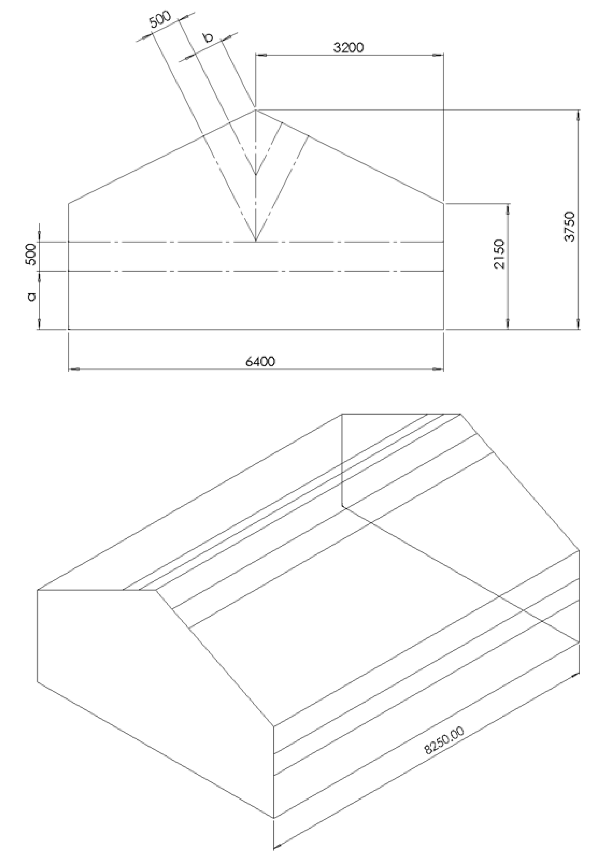
Figure 1. A cross-section of the greenhouse (GH) geometry used in the simulations for the 2D and 3D models (Dimensions in mm).
Sustainability 12 00986 g001
Figure 2. Planes used to analyse the 3D model.
Sustainability 12 00986 g002
Figure 3. The air-flow pattern, temperature contour and water vapour contour of the initial 2D model.
Sustainability 12 00986 g003
Figure 4. Air-flow pattern, temperature contour and water vapour contour of the initial 3D model for the centre of the GH.
Sustainability 12 00986 g004
Figure 5. Air-flow pattern, temperature contour and water vapour contour of the initial 3D model from a top view, where the plane is raised 1.25 m to coincide with the centre of the vent.
Sustainability 12 00986 g005
Figure 6. Air-flow pattern, temperature contour and water vapour contour of the model with side vents located 0.25 m above the floor of the GH.
Sustainability 12 00986 g006
Figure 7. Air-flow pattern, temperature contour and water vapour contour of the model with side vents located 1.50 m above the floor of the GH.
Sustainability 12 00986 g007
Figure 8. Air-flow pattern and temperature contour of the model with roof vents located 3.00 m from the ridge of the GH.
Sustainability 12 00986 g008
Figure 9. Air-flow pattern and temperature contour of the model with no roof vents and side vents located 1.00 m above the floor of the GH.
Sustainability 12 00986 g009aSustainability 12 00986 g009b
Figure 10. The air velocity plotted against the vertical distance from the ground at the centre of the (a) GH Figure 0.5 m from the ridge, (b) a GH with roof vents 2.00 m from the ridge, (c) a GH with roof vents 3.00 m from the ridge.
Sustainability 12 00986 g010
Figure 11. The air-flow pattern of the model with no roof vents and side vents located 0.50 m above the floor of the GH.
Sustainability 12 00986 g011
Figure 12. Air-flow pattern, temperature contour and water vapour contour of the model with no side vents and roof vents located 0.50 m from the ridge of the GH.
Sustainability 12 00986 g012aSustainability 12 00986 g012b
Figure 13. Temperature plotted against the vertical distance from the floor at the centre of the GH for (a) a GH with side vents 1.00 m above the ground—the initial model, (b) a GH with side vents 0.50 m above the ground and no roof vents, (c) a GH with side vents 1.00 m above the ground and no roof vents, (d) a GH with side vents 1.50 m above the ground and no roof vents.
Sustainability 12 00986 g013
Figure 14. Air-flow pattern, temperature contour and water vapour contour of the model with no side vents and roof vents located 3.00 m from the ridge of the GH.
Sustainability 12 00986 g014
Figure 15. The air-flow pattern of the initial model with an external wind speed of 0.6 m/s.
Sustainability 12 00986 g015
Figure 16. A graph showing the ratio (air velocity through vent/ external wind speed) for the four wind speed cases studied.
Sustainability 12 00986 g016
Figure 17. The temperature plotted against the vertical distance from the ground at the centre of the GH for floor temperatures of (a) 310 K, (b) 315 K, (c) 320 K (initial model), (d) 325 K.
Sustainability 12 00986 g017
Figure 18. The temperature plotted against the horizontal distance from the windward vent at a height of 1.00 m for (a) a GH with side vents 0.25 m above the ground, (b) a GH with side vents 1.00 m above the ground, (c) a GH with side vents 1.50 m above the ground.
Sustainability 12 00986 g018
Table 1. The dimensions of the greenhouse (GH) and external air used for the Computational Fluids Dynamics (CFD) geometry.
DimensionValue
Length8.25 m
Width6.40 m
Ridge Height3.75 m
Eaves Height2.15 m
Side Ventilator Vertical Length0.50 m
Side Ventilator Height (above ground)a
Roof Ventilator Vertical Length0.50 m
Roof Ventilator Distance from Ridgeb
External Upstream Air Length2.00 m
External Downstream Air Length8.00 m
External Air Height5.00 m
Table 2. The material properties used in the simulation for glass and soil [46].
MaterialDensity (kg/m3)Specific Heat (J/kgK)Thermal Conductivity (W/mK)
Glass24007531.0
Soil22008710.5
Table 3. The boundary conditions used in the 2D model [65].
Named SelectionBoundary TypeBoundary Conditions
GH WallsWall (glass)T = 310 K
GH RoofWall (glass)T = 310 K
GH FloorWall (soil)T = 320 K
External FloorWall (soil)T = 300 K
InletVelocity-inletU = 0.2 m/s
T = 300 K
OutletPressure-outletN/A
External RoofSymmetryN/A
Table 4. The boundary conditions used in the 3D model. Note: ‘end’ refers to the walls perpendicular to the GH ridge axis, whilst ‘side’ refers to the walls parallel to the GH ridge axis [65].
Named SelectionBoundary TypeBoundary Condition(s)
GH Side WallsWall (glass)T = 310 K
GH End WallsWall (glass)T = 310 K
GH RoofWall (glass)T = 310 K
GH FloorWall (soil)T = 320 K
External FloorWall (soil)T = 300 K
External WallsWall (glass)T = 310 K
InletVelocity-inletU = 0.2 m/s
T = 300 K
OutletPressure-outletN/A
External RoofSymmetryN/A
Table 5. The convergence study for the optimal number of elements.
MeshNumber of ElementsAverage
Horizontal
Velocity (m/s)
Average
Horizontal
Temperature (K)
Average
Vertical
Velocity (m/s)
Average
Vertical
Temperature (k)
183370.116304.740.200305.31
233,2360.101304.870.188305.29
345,6920.217303.930.173304.47
461,4200.227304.240.187304.71
563,3040.083304.390.180304.68
678,5010.220304.330.187304.79
790,8150.153304.200.161304.65
8101,7270.132304.230.160304.67
9107,4170.082305.800.212305.44
10116,6690.219304.310.178304.78
11206,0080.154304.220.160304.66
12214,4040.210303.900.185304.53
13227,1260.213304.170.184304.70
14272,0450.212304.920.197305.23
15372,9990.168304.060.196304.53
16379,4390.180304.270.198304.65
17419,4900.204304.650.215305.03
18486,9470.180304.080.182304.55
19503,4490.187304.220.201304.64
20571,7260.175304.160.173304.54
21586,4550.161304.440.195304.73
22679,9250.171304.180.159304.48
23696,4380.161304.350.173304.56
24819,8620.158304.180.143304.40
25835,5340.148304.300.147304.51
26877,8060.151304.660.155304.69

