Quantitative Assessment for the Dynamics of the Main Ecosystem Services and their Interactions in the Northwestern Arid Area, China

Abstract

Evaluating changes in the spatial–temporal patterns of ecosystem services (ESs) and their interrelationships provide an opportunity to understand the links among them, as well as to inform ecosystem-service-based decision making and governance. To research the development trajectory of ecosystem services over time and space in the northwestern arid area of China, three main ecosystem services (carbon sequestration, soil retention, and sand fixation) and their relationships were analyzed using Pearson’s coefficient and a time-lagged cross-correlation analysis based on the mountain–oasis–desert zonal scale. The results of this study were as follows: (1) The carbon sequestration of most subregions improved, and that of the oasis continuously increased from 1990 to 2015. Sand fixation decreased in the whole region except for in the Alxa Plateau–Hexi Corridor area, which experienced an “increase–decrease” trend before 2000 and after 2000; (2) the synergies and trade-off relationships of the ES pairs varied with time and space, but carbon sequestration and soil retention in the most arid area had a synergistic relationship, and most oases retained their synergies between carbon sequestration and sand fixation over time. Most regional relationships of sand fixation and soil retention with a weak trade-off during the before-2000 stage turned into weak synergies at the after-2000 stage; (3) the ES pairs of carbon sequestration and sand fixation had significant time-lagged trade-off relationships in most arid areas, and these time trade-offs were generally maintained for 2–6 years, where a higher absolute value of the maximum time-lagged correlation coefficient corresponded to a longer time-lag. This study could assist us in understanding the trade-off and synergy of ESs and will provide quantitative zonal information for the ecosystem-services-based ecomanagement of arid areas.

1. Introduction

Ecosystem services (ESs) are defined as the benefits of the natural environment that sustain the survival of people and the products and services directly or indirectly through ecosystem functions. These services contribute greatly to human welfare and goods [1]. Generally, ESs fall into four main categories: provisioning services, supporting services, regulating services, and cultural services [2]. Lower-level classifications (widely recommended by previous research) include the system of Costanza et al. [3] and the scheme of Xie et al. [4].

To date, numerous prior studies have researched changes in ESs, potential factors of these changes, and the interrelations among ESs. Approaches to quantifying ESs comprise two main categories: the economic value of ESs and physical materialization. The selection of methods is generally dependent on the objective of the assessments. The former mainly includes the earliest monetization of ESs [1,5], evaluation methods based on the value equivalent factor in the unit area [6], and the function valuation method. The latter mainly consists of surrogate models that have emerged in the last decade (e.g., models based on net primary production (NPP) [7,8,9], energy flow, or carbon flow [10]), and the recent integrated models from multiple biophysical process simulations (e.g., InVEST (integrated valuation of ecosystem services and trade-offs) and SolVES (social values for ecosystem services)) [11,12,13]. Both methods need accurate estimates of the parameters. Economic value methods require measure equivalent coefficients, and physical materialization methods should be satisfied with local adaptive parameters. Regardless of the quantitative method applied, similar conclusions are drawn: Assessing changes in ecosystem services has become crucial for current environment policies [2,14]. The diversity of ESs, spatial heterogeneity, and the selectivity and diversity of management has led to the trade-offs and synergies of ES pairs [15,16]. Trade-offs refer to interactions whereby one ES restrains another, and synergy refers to mutual enhancement. These studies deepen and enrich our understanding of ESs and ecosystem complexity but also guide us to determine the mechanisms of interactions among ESs. Generally, researchers have focused on the spatial interactions among ESs—that is, the relationship between multiple ESs of one region. However, there are also temporal trade-offs and temporal synergies among them [17]. The characteristics of ES dynamics and the interrelationships among them are increasingly considered to be pivotal in ecological conservation and restoration, land-use management, urban planning, and the assessment of ecosystem sustainability [2,18,19].

The aforementioned reasons triggered our interest in evaluating the dynamics of ESs in the northwestern arid area of China (NW) and investigating changes in their interactions over space and time. This area fosters around 2487 million people, and all of them receive ecosystem services from this extremely fragile and further deteriorating ecological environment. Structural damages to the regional ecosystem and the ecosystem’s functional chaos are inhibiting society and economically sustainable development and hindering people from escaping poverty. Following the announcement of China’s central government, nationally widespread ecological restoration programs were launched, such as the Grain for Green Program, Returning Livestock Pastures to Natural Grasslands, Natural Forest Protection Project, Comprehensive Control of Desertification Area Project, and Shelter Forest Project in North, Northeast, and Northwest China. The people of the NW have actively taken part in these programs and have conducted a series of ecological conservation, repair, and reconstruction efforts, such as the Tianshan Mountains–Altai Mountains Natural Forest Protection Project in 2000, the comprehensive ecological improvements in the Tarim River basin and its environs in 2000, the extensive afforestation of Karamay in 2002, and the prevention and control of desertification in the Junggar Basin in 2010. Under these combined effects, the ecosystem’s quality and structure have partially improved, as evidenced by the presentation of the normalized differential vegetation index (NDVI) [20], leaf area index (LAI) [21], and fraction of vegetation coverage, notwithstanding the spatial heterogeneity of their changes.

Here, three questions were proposed: How do ecosystem services change? What is the development trajectory of these ecosystem services over time? What can policymakers do to improve each ecosystem-service-based current condition? This paper attempts to answer these questions using the following three approaches: (1) zonally comparing the dynamics of carbon sequestration, soil retention, and sand fixation from the time and space dimensions; (2) detecting the spatial distribution and temporal trends of the interactions (including trade-offs and synergies) among ESs using Pearson’s correlation coefficient; and (3) revealing the time-lagged effects among ESs based on a time-lagged cross correlation analysis. Based on the most striking ecological environment issues (vegetation degradation, soil erosion, and desertification) and high spatial resolution data availability, as well as carbon sequestration, soil retention, and sand fixation, these three ESs were selected to be assessed. According to the assessment results, clarifying the regional difference among ESs and their relationships helps establish a reference case for creating win–win strategies of zonal development and the ecological protection of arid areas.

2. Materials and Methodology

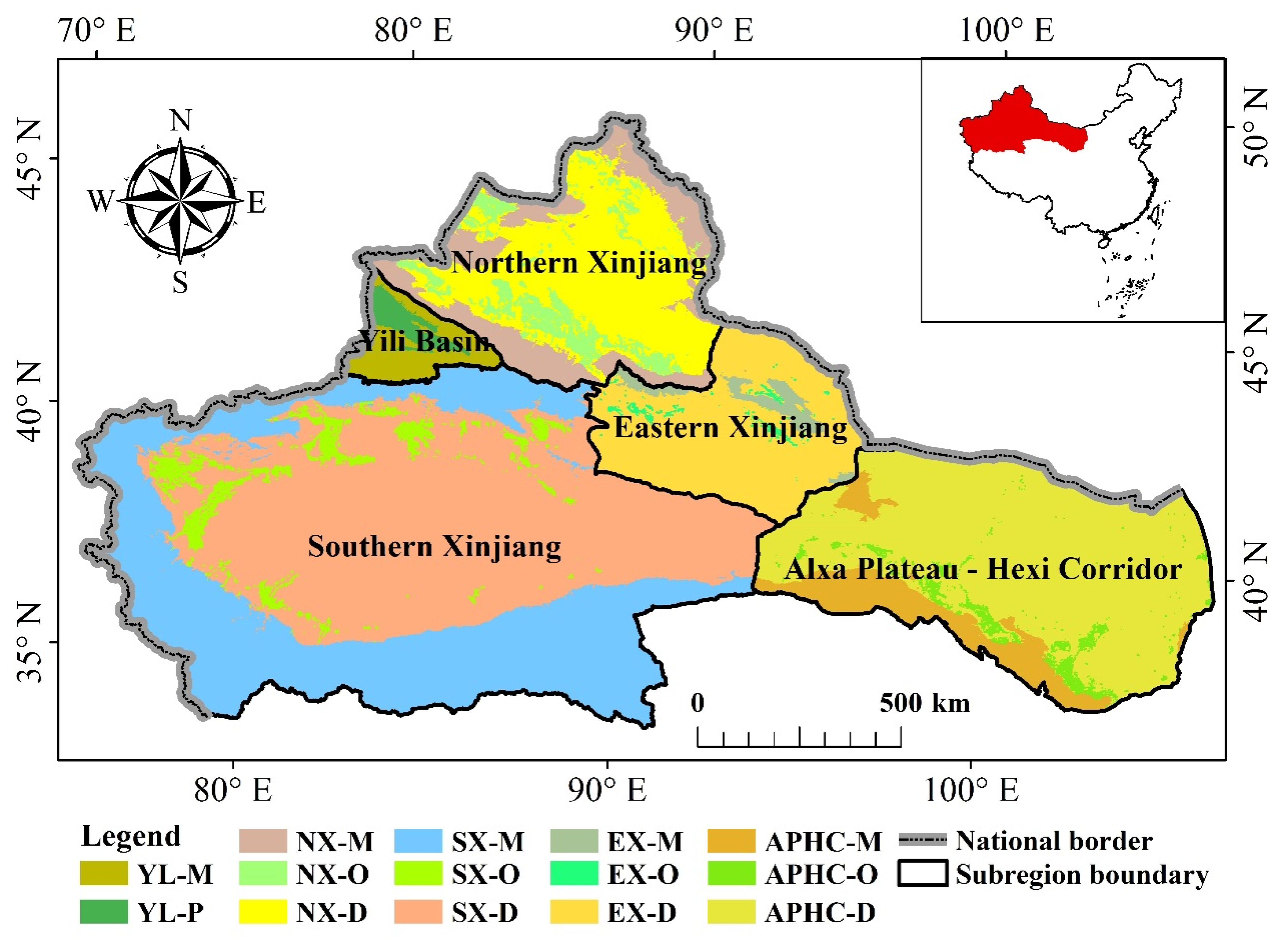
2.1. Study Area

The northwestern arid area of China (34°20′10″ N ~ 49°10′30″ N, 73°33′27″E ~ 106°50′34″ E) lies to the north of the Kunlun Mountains–Qilian Mountains terrain belt and to the west of the Helan Mountains, with an area of 235 × 10⁴ km², around one quarter the size of China. This arid area includes the whole area of the Xinjiang Uygur Autonomous Region, the Alxa plateau of the Inner Mongolia Autonomous Region, and the Hexi corridor (i.e., towards the west of the Yellow River) of Gansu province, with a total of 134 counties. The study area has a temperate continental climate, except for high-altitude localities with highland mountain climates. Here, the strong evapotranspiration capability is 8~10 times as great as its extremely scarce precipitation (230 mm). Mountain ranges (M) surround the two basins, and extensive deserts (D) are interwoven with scattered oases (O), a unique type of topography denoted a mountain–oasis–desert system (MODS). Referring to the research of Wang et al. [22], our study divides the northwestern arid land into five large parts: northern Xinjiang (NX), southern Xinjiang (SX), the Yili basin (YL), eastern Xinjiang (EX), and the Alxa Plateau–Hexi Corridor area (APHC). Furthermore, mountains, oases, and deserts are extracted for each area based on the elevation range and land use type. Here, Yili is only zoned into mountains and plains. After these partitions, the study area is divided again into 14 sub-regions (Figure 1).

2.2. Data and Preprocessing

Meteorological observations of the 86 stations in and around the study area were collected from the National Meteorological Information Center (http://data.cma.cn/). The meteorological elements include daily wind speed, maximum air temperature, minimum air temperature, sunshine hours, relative humidity, and precipitation. After removing outliers (about 0.1%), the daily meteorological data over a half month and a whole month were averaged from records at day 15 and day 30 of the corresponding month. By applying AUNSPLIN 4.3, half-monthly and monthly grid meteorological data (5 km × 5 km) were generated by spatial interpolation. The Shuttle Radar Topographical Mission (SRTM) digital elevation model (DEM) data, with a 3 arc-second spatial resolution, was download from the Resource and Environment Data Cloud Platform (http://www.resdc.cn/). The gridded data of the soil particle diameter fraction was generated by the National Second Soil Survey of China, whose units were transformed from International Units (clay, silt, and sand: 0.002–0.02–2.000 mm) into American Units (clay, silt, and sand: 0.002–0.050–2.000 mm) using the Logarithmic normal distribution function. Besides soil texture data, the land cover map from the Climate Change Initiative (https://www.esa-landcover-cci.org/) (CCI-LC, v2.0), snow depth data (http://westdc.westgis.ac.cn/), and the LTDR (Land Long Term Data Record) v5 NDVI (https://ltdr.modaps.eosdis.nasa.gov/) were resampled into a 5 km × 5 km spatial solution.

2.3. Methods

2.3.1. Carbon Sequestration

In this study, NPP (gC·m⁻²·a⁻¹) was selected as an indicator of carbon sequestration ESs. The terrestrial Carnegie Ames-Stanford Approach (CASA) model [23] was used to estimate NPP based on a light-use efficiency model. Compared with other NPP-models based on biophysical processes (e.g., VPM (Vegetation Photosynthesis Model) [24], BESS (Breathing Earth System Simulator Model) [25], and GLO-PEM (Global Production Efficiency Model) [26]), CASA demands fewer inputs and consumes less time for computing due to its simple and efficient algorithm. Its formulations are as follows:

$$NPP\left(x,t\right)=APAR\left(x,t\right)\times \epsilon \left(x,t\right)$$

(1)

$$APAR\left(x,t\right)=SOL\left(x,t\right)\times FPAR\left(x,t\right)\times 0.5$$

(2)

$$\epsilon \left(x,t\right)={\epsilon }_{\max }\times T_{\epsilon 1}\left(x,t\right)\times T_{\epsilon 2}\left(x,t\right)\times W_{\epsilon }\left(x,t\right)$$

(3)

where APAR(x,t) is the photosynthetically absorbed active radiation (MJ·m⁻²) on the grid cell x in month t; ε is the light-use efficiency (gC·MJ⁻¹) of the vegetation at location x at time t; SOL is the total solar radiation (MJ·m⁻²); and FPAR is the fraction of the photosynthetically active radiation absorbed by the canopy. Light-use efficiency refers to the canopy’s efficiency in transforming absorbed radiation into organic carbon, as a process controlled by low temperature, high temperature, and wetness. Therefore, ε is allowed to be represented by the stress of low temperature and high temperature (T_ε1), the stress effects of the gap between the varying ambient air temperature, and the optimal temperature closely related to the accumulation of NPP (T_ε2), as well the wetness stress (W_ε). These three variables are dimensionless. ε_max is the maximum possible efficiency. Here, the studies of Jiao Wei et al. [27] and Zhu Wenquan et al. [28] serve as the main references to calculate the key parameters (i.e., NDVImax, NDVImin, SRmax, SRmin, and ε_max) based on the 16 reclassified land-cover types and 8 land-use types from the CCI-LC map.

2.3.2. Soil Retention

The Revised Universal Soil Loss Equation (RUSLE) was employed to calculate soil retention. It can be formulated as

$$SC=S{E}_P-S{E}_V=R\times K\times L\times S\times \left(1-C-P\right)$$

(4)

where SC, SE_P, and SE_V represent the soil’s retention capacity (t·km⁻²·a⁻¹), potential soil loss (t·km⁻²·a⁻¹), and actual soil loss (t·km⁻²·a⁻¹), respectively; R is the rainfall erosivity factor (MJ·mm·km⁻²·h⁻¹·a⁻¹); K is the soil erodibility factor (t·km²·h·km⁻²·MJ⁻¹·mm⁻¹); L, S, C, and P are the slope length factor, slope factor, vegetation factor, and management factor, and all factors are dimensionless. The value of P can be retrieved from different land use/covers and slopes. In this study, a reformulated scheme of the rainfall erosion factor from Yang Fengbo and Lu Changhe’s study [29] was used to compute the R of the study area, which is described as

$$R=a{{\displaystyle \sum _{j=1}^k\left(P_j\right)}}^{\beta }$$

(5)

$$\beta =0.8363+\frac{18.144}{P_{d12}}+\frac{24.455}{P_{y12}}$$

(6)

$$a=17.554\times {\beta }^{-7.042}$$

(7)

where R is the rainfall erosivity in a half month (MJ mm ha⁻¹ h⁻¹), P_j is the erosive rainfall (mm) for day j in a given half-month, and α and β are the empirical coefficients that are practical for the northern area of China. P_d12 and P_y12 are the average daily and annual rainfall for the days with rainfall ≥12 mm. The annual erosivity is the summation of all half-month erosivity during the year.

$$\begin{array}{l}K=\left[0.2+0.3\times e^{-0.0256\times sand\times \left(1-silt/100\right)}\right]\times {\left(\frac{silt}{clay+silt}\right)}^{0.3}\\ \times \left[1-\frac{0.25\times oc}{toc+e^{3.72-2.95\times toc}}\right]\times \left[1-\frac{0.7\times sni}{sni+e^{22.9\times sni-5.51}}\right]\times 0.13\end{array}$$

(8)

where sand, silt, clay, and oc are the content fraction of sand, silt, clay, and organic carbon in the top soil layer (%); sni = 1 − sand/100.

$$L={\left(\frac{\lambda }{22.13}\right)}^m,\{\begin{array}{l}m=0.5,\theta \ge 9\\ m=0.4,3\le \theta <9\\ m=0.3,1\le \theta <3\\ m=0.2,\theta <1\end{array}$$

(9)

$$S=\{\begin{array}{cc}10.8\sin \theta +0.03\hspace{1em}\hfill & \theta {<5}^{°}\\ 16.8\sin \theta -0.50\hfill & 5^{°}\le \theta \le {10}^{°}\\ 21.9\sin \theta -0.96\hfill & \theta \ge {10}^{°}\end{array}$$

(10)

$$C=\{\begin{array}{cc}1\hfill & fvc=0\\ 0.6508-0.3436\times \lg fvc\hfill & 0<fvc\le 78.3\%\\ 0\hfill & fvc>78.3\%\end{array}$$

(11)

where λ, θ, and m are the slope length, slope, and slope index, respectively, while fvc is the vegetation coverage.

2.3.3. Sand Fixation

The Revised Soil Erosion Equation (RWEQ) model was used to simulate the regional wind erosion modulus (defined as the soil loss per unit area) [30] of the northwestern arid area of China. This model combines empirical and process modeling and has been extensively tested under broad field conditions [11,13,14].

$$S{T}_{\max 0}=109.8[\mathrm{WF}\times \mathrm{EF}\times \mathrm{SCF}\times {\mathrm{K}}^{\prime }]$$

(12)

$$S_0=150.71\left(WF\times EF\times SCF\times K^{\prime }\right)-0.3711$$

(13)

$$S{L}_0=\frac{2z}{S_0^2}S{T}_{\max 0}\cdot e^{-{(z/s_0)}^2}$$

(14)

where ST_{max 0} is the maximum transport capacity (kg/m), WF is the climatic factor (kg/m), EF is the soil erodibility factor (%), SCF is the soil crust factor (dimensionless), K′ is the surface roughness (dimensionless), S₀ is the field length scale (m), and Z is the distance from the upwind edge of the field (m).

ST_max = 109.8[WF × EF × SCF × K′ × VEG]

(15)

$$S=150.71\left(WF\times EF\times SCF\times K^{\prime }\times VEG\right)-0.3711$$

(16)

$$SL=\frac{2z}{S^2}S{T}_{\max }{e}^{-{(z/s)}^2}$$

(17)

$$SF=S{L}_0-SL$$

(18)

where VEG is the vegetation coverage factor; S is the critical field length, at which 63% of maximum transport capacity occurs. SF (sand fixation (t·hm⁻²·a⁻¹)) is the difference between potential soil erosion (SL₀, t·hm⁻²·a⁻¹) and actual soil erosion (SL, t·hm⁻²·a⁻¹) per unit area by wind.

2.3.4. Trend Analysis

The linear slopes of the analytical factors (carbon sequestration, soil retention, and sand fixation) over time can reflect changing trends. The slope of the linear model was calculated for each ES at every time period (1990–2000, 2000–2015, and 1990–2015) by using the regress function of MATLAB R2016a. The formulas are as follows:

yi = α + βxi + εi

(19)

$$\alpha =\frac{{\displaystyle \sum _{i=1}^n\left(xi-\overline{x}\right)\left(yi-\overline{y}\right)}}{{\displaystyle \sum _{i=1}^n{\left(xi-\overline{x}\right)}^2}}$$

(20)

where xi is the i_th value of the ES time series for a certain time period, and n is the total number of years for a certain time period. A negative value of slope (α) represents the occurrence of a decrease, while a positive value of the slope means an increasing trend. Meanwhile, a t-test was used to identify the linear significance.

2.3.5. Correlation Analysis

To uncover the relationships of the ESs, a Pearson’s correlation analysis (using the corr function in MATLAB R12a) was conducted among the pairs of ESs for each time period (1990–2000, 2000–2015, and 1990–2015). A positive correlation coefficient indicates that paired ESs have a synergistic relationship, whereas a negative correlation coefficient indicates a certain trade-off between the paired ESs.

2.3.6. Time-Lagged Cross-Correlation Analysis

A time-lagged cross correlation analysis was used to research the interaction time of each ES pair. With the assumption that every ESs pair is related to all other pairs at any time-lagged point, their time-lagged correlation coefficient can be represented as

$$r_k\left(x,y\right)=c_k\left(x,y\right)/\left({\delta }_x{\delta }_{y+k}\right)$$

(21)

where r_k is the correlation coefficient at time-lagged point k, c_k is the covariance of time series x_t and time series y_t+k, δ_x is the mean square deviation of time series x_t, and δ_y+k is the mean square deviation of time series y_t+k. These statistical parameters are calculated as follows:

$$\{\begin{array}{c}{c}_k\left(x,y\right)=\frac{1}{n-k}{\displaystyle \sum _{t=1}^{n-k}\left(x_t-\overline{x_t}\right)}\left(y_{t+k}-\overline{y_{t+k}}\right)\\ {\delta }_x=\sqrt{\frac{1}{n-k}{\displaystyle \sum _{t=1}^{n-k}\left(x_t-\overline{x_t}\right)}}\\ {\delta }_{y+k}=\sqrt{\frac{1}{n-k}{\displaystyle \sum _{t-1}^{n-k}\left(y_{t+k}-\overline{y_{t+k}}\right)}}\end{array}$$

(22)

where the time-lagged k is equal to 0, ±1, ±2, …, ±n/4; $\overline{y_{t+k}}$ is the mean of the time-lagged series y_t+k, and $\overline{x_t}$ is the mean of time series x_t.

3. Results

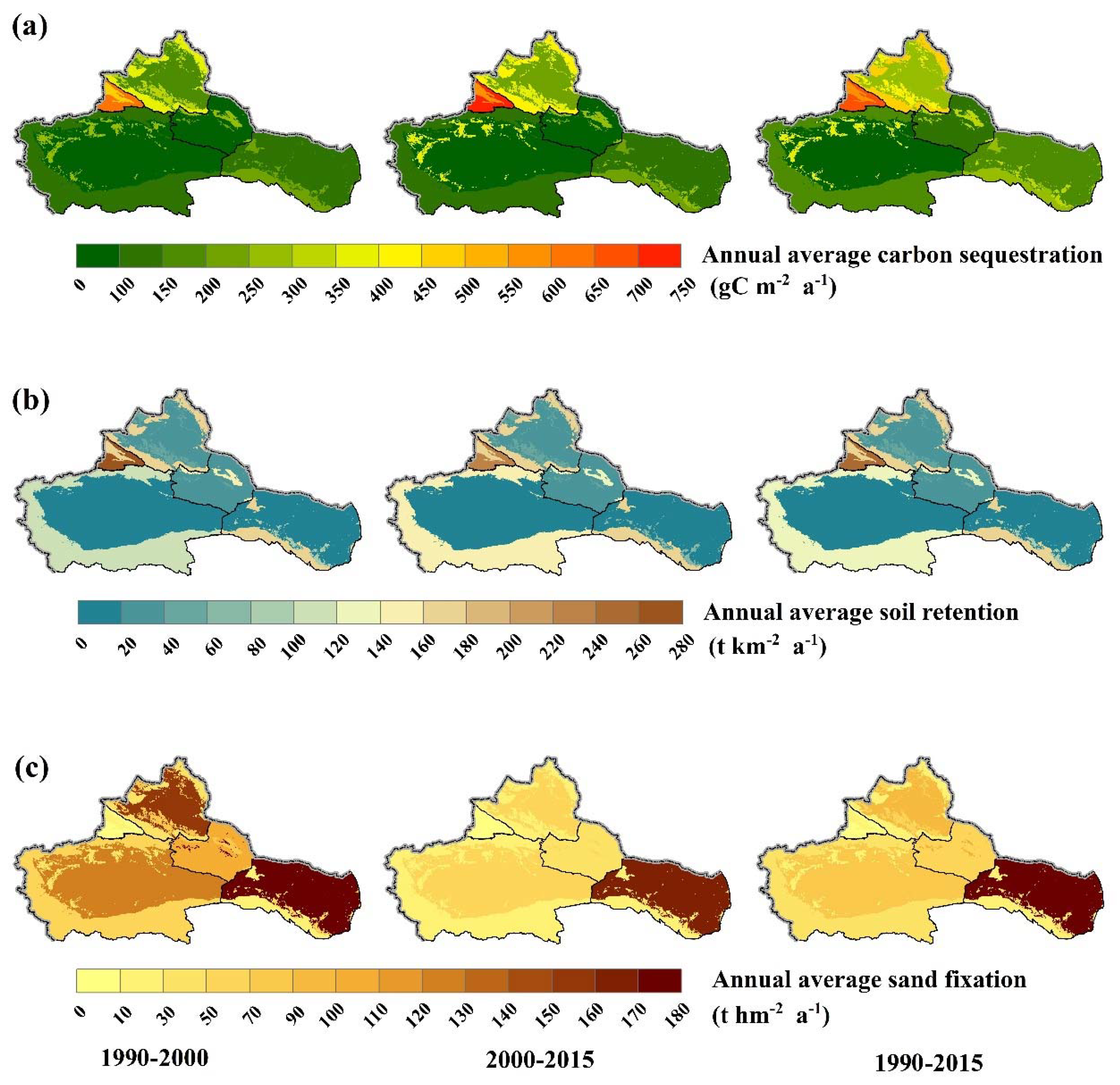
3.1. Spatial Pattern and Temporal Trends of ESs

The ecosystems services of NW from 1990 to 2015 had an average of 159.563 gC m⁻² a⁻¹, 70.077 t km⁻² a⁻¹, and 80.256 t hm⁻² a⁻¹ in annual carbon sequestration, soil retention, and sand fixation, respectively. The spatial patterns of the ecosystem services during the two sub-periods (i.e., before 2000 and after 2000) and over the whole study period are shown in Figure 2. Carbon sequestration during these time periods represented a similar spatial pattern (Figure 2a). Among all MODS sub-regions, the Yili mountains had the highest carbon sequestration regardless of time period (before 2000: 559.567 gC m⁻² a⁻¹; after 2000: 678.577 gC m⁻² a⁻¹; 1990–2015: 638.300 gC m⁻² a⁻¹), and the southern Xinjiang deserts always had the lowest carbon sequestration (before 2000:83.446 gC m⁻² a⁻¹; after 2000: 76.269 gC m⁻² a⁻¹; 1990–2015:77.771 gC m⁻² a⁻¹). Obviously, the northern Xinjiang oasis and mountains and southern Xinjiang oasis had higher carbon sequestration than the other MODS sub-regions of NW. Soil retention distinctively varied across the whole arid area (Figure 2b). Soil retention during these three periods had similar spatial patterns. As in the ranking of carbon sequestration, among the 14 sub-regions, the Yili mountains experienced the highest soil retention (1990–2000: 265.306 t km⁻² a⁻¹; 2000–2015: 237.099 t km⁻² a⁻¹; 1990–2015: 242.067 t km⁻² a⁻¹). However, the southern Xinjiang oasis and its desert, as well as the Alxa Plateau–Hexi Corridor desert, had the lowest soil retention. Besides being the highest and the lowest areas, the northern Xinjiang mountains, Alxa Plateau-Hexi Corridor mountains, and Yili plains experienced higher soil retention. In a word, most mountains had higher soil retention than deserts and oases. The boundary between the soil retention of the desert and that of the oasis, therefore, seems to disappear. As shown in Figure 2c, the highest value of the sand fixation was concentrated on the Alxa Plateau–Hexi Corridor in all periods (before 2000: 150.805 t hm⁻² a⁻¹; after 2000: 139.966 t hm⁻² a⁻¹; 1990–2015: 141.685 t hm⁻² a⁻¹). Before 2000, the spatial distribution of sand fixation displayed an obvious difference. At this time, sand fixation of the northern Xinjiang deserts had a higher magnitude (159.154 t hm⁻² a⁻¹). For the other two time periods, there was little spatial difference in the sand fixation of Xinjiang.

Least-squares linear regression was used to predict the slope of each ES in every sub-region for different periods (

Table 1. Estimates of the linear regression model for the ESs of each sub-region at time periods 1990–2000, 2000–2015, and 1990–2015. The units of the slope of carbon sequestration, soil retention, and sand fixation are gC m⁻² a⁻², t km⁻² a⁻², and t hm⁻² a⁻², respectively.

Ecosystem Services	Regions	Before 2000		After 2000		1990–2015
		Slope	p	Slope	p	Slope	p
Carbon sequestration	NX-M	−3.307	0.209	−4.853	0.160	−2.029	0.134
	NX-O	−1.598	0.133	−0.788	0.357	−0.462	0.201
	NX-D	−1.383	0.063	−0.601	0.312	−0.348	0.170
	SX-M	6.123	0.165	−3.725	0.619	2.981	0.309
	SX-O	0.592	0.275	0.243	0.475	0.080	0.602
	SX-D	0.453	0.503	−0.191	0.733	−0.006	0.980
	EX-M	−8.825	0.071	−3.761	0.528	−2.113	0.367
	EX-O	−3.097	0.075	−0.797	0.661	−0.671	0.359
	EX-D	−1.990	0.127	−1.151	0.451	−0.640	0.286
	APHC-M	0.034	0.996	−1.231	0.720	0.245	0.889
	APHC-O	1.694	0.631	−0.329	0.791	−0.085	0.909
	APHC-D	−0.198	0.747	0.045	0.894	−0.069	0.664
	YL-M	7.104	0.455	−6.830	0.175	−1.769	0.467
	YL-P	2.813	0.589	−5.064	0.171	−1.107	0.493
Soil retention	NX-M	−3.307	0.209	−4.853	0.159	−2.029	0.134
	NX-O	−1.599	0.133	−0.788	0.357	−0.463	0.201
	NX-D	−1.383	0.063	−0.601	0.311	−0.348	0.170
	SX-M	6.123	0.165	−3.725	0.619	2.981	0.309
	SX-O	0.592	0.275	0.243	0.474	0.080	0.602
	SX-D	0.453	0.503	−0.191	0.733	−0.006	0.980
	EX-M	−8.825	0.071	−3.761	0.528	−2.113	0.367
	EX-O	−3.097	0.075	−0.797	0.661	−0.671	0.359
	EX-D	−1.910	0.127	−1.151	0.45	−0.640	0.286
	APHC-M	0.0340	0.996	−1.231	0.720	0.245	0.889
	APHC-O	1.694	0.631	−0.329	0.791	−0.085	0.909
	APHC-D	−0.198	0.747	0.045	0.894	−0.069	0.664
	YL-M	7.104	0.455	−6.830	0.175	−1.769	0.467
	YL-P	2.813	0.589	−5.064	0.171	−1.107	0.493
Sand fixation	NX-M	−2.677 **	0.004	−1.493 **	0.001	−2.098 **	9 × 10−12
	NX-O	−7.407 **	0.001	−4.005 **	0.001	−4.826 **	1 × 10−10
	NX-D	−10.446 **	0.009	−6.281 **	0.002	−8.219 **	1 × 10−9
	SX-M	−2.555	0.079	−1.919 **	0.009	−2.382 **	9 × 10−8
	SX-O	0.095	0.913	−1.036	0.128	−1.091 **	0.001
	SX-D	0.007	0.997	−5.913 **	0.001	−4.863 **	2 × 10−7
	EX-M	−4.167	0.093	−3.134 **	0.002	−4.069 **	1 × 10−8
	EX-O	−12.300 *	0.011	−7.989 **	3×10-5	−9.428 **	4 × 10−11
	EX-D	−4.988 *	0.043	−3.905	0.001	−5.159 **	4 ×10−10
	APHC-M	0.366	0.723	−0.629	0.141	−0.613 *	0.014
	APHC-O	0.812	0.518	−2.147 *	0.034	−0.778	0.063
	APHC-D	7.310*	0.018	−8.380 **	0.003	−1.894	0.120
	YL-M	−0.292	0.663	−0.095	0.532	−0.229	0.069
	YL-P	−0.717	0.652	−0.202	0.525	−0.609 *	0.041

Note: the * symbol on the top-right of the p value means that the tendency is significant (p < 0.05), and the ** symbol means that the tendency is very significant (p < 0.01).

, Figure 3). In terms of carbon sequestration, the whole arid area, mountains, and desert had similar temporal trends: The before-2000 series significantly increased (p < 0.01), and the after-2000 series significantly decreased (p < 0.05), with a slight variation over the whole period. Carbon sequestration of the oasis significantly increased during all periods. Carbon sequestration of the MODS for each large region resembled that of the MODS for the whole NW (mountains: increase–decrease; oasis: increase–increase; desert: increase–decrease) in the two sub-periods (Table 1, Figure 3(a1–a3)). In terms of soil retention, although the regional average of the oases and deserts decreased, the average increased in the mountains and for the whole NW during 1990–2015 (Figure 3(b1–b3)). None of the trends of these regional averages passed a significance level of a = 0.05. As Table 1 details, during 1990–2015, soil retention of the oasis and deserts in SX, EX, APHC, and YL increased, but that of the MODS sub-regions in the NX decreased (Table 1). Before 2000, the soil retention of mountains and oases in all five large regions slightly declined, except for the MODS of NX, which showed increasing trends. After 2000, the soil retention of all MODS sub-regions insignificantly decreased, except for SX-O and APHC-D, which showed increasing trends. In terms of the sand fixation, mountains, oases, deserts, and the whole arid area all showed a monotonous downward trend (p < 0.01) during 1990–2015, with a slope of −2.080 t hm⁻² a⁻², −2.591 t hm⁻² a⁻², −4.535 t hm⁻² a⁻², and −3.666 t hm⁻² a⁻², respectively. Although most MODS sub-regions experienced significant upward trends during the whole study period, when viewed by the two sub-periods, half of the MODS sub-regions in the entire NW area (i.e., the MODS of NX, EX and YL, and SX-M) continuously decreased, while the other half (i.e., the MODS of APHC, SX-O, and SX-D) experienced an increase–decrease process (Table 1, Figure 3(c1–c3)).

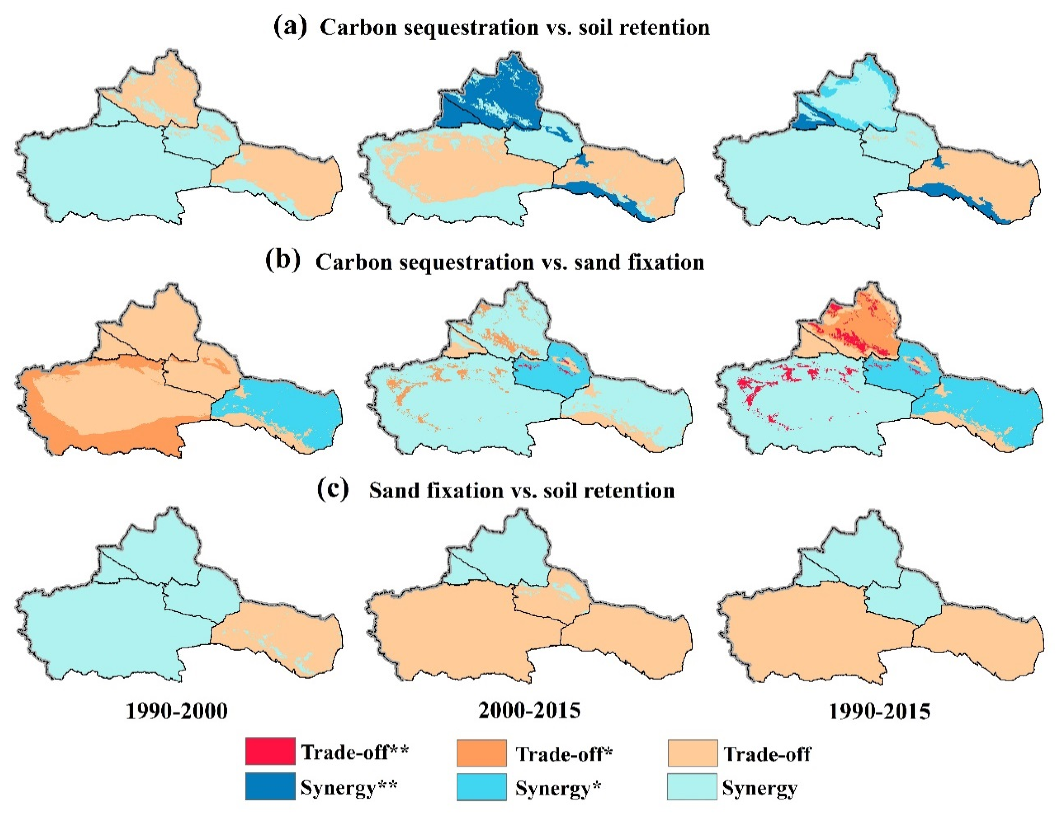
3.2. Spatial Patterns and Temporal Trends of the Relationships between ES Pairs

The interactions determined by regional average correlation coefficients are shown in Figure 4, alongside those that were checked according to significance (p < 0.05). The relationships between carbon sequestration and soil retention, carbon sequestration and sand fixation, and sand fixation and soil retention were classified into six categories: trade-off** (r < 0, p ≤ 0.01), synergy** (r > 0, p ≤ 0.01), trade-off*(r < 0, 0.01 < p ≤ 0.05), synergy* (r > 0, 0.01 < p ≤ 0.05), trade-off (r < 0, p > 0.05), and synergy (r > 0, p > 0.05). These trade-offs and synergies (Figure 4) have great spatial and temporal heterogeneity throughout the whole NW. From the aspect of the relationship between carbon sequestration and soil retention, during 1990–2015, synergies were present in all sub-regions of NW, except APHC-D, with a strong trade-off (r < 0, p ≤ 0.05) (Figure 4a). Before 2000, weak synergies (r > 0, p > 0.05) were mostly spread across the whole arid area, with the exception of weak trade-offs (r < 0, p > 0.05) in the NX-D, EX-O, and APHC-D. After 2000, only SX-D and APHC-D had a weak trade-off relationship, while the other sub-regions established synergistic relationships between carbon sequestration and soil retention, which presented all the strong synergies for the oases and the whole YL (r > 0, p ≤ 0.05). From the perspective of the relationship between carbon sequestration and sand fixation, during 1990–2015, trade-offs occurred in all oases (including YL-P), and the majority of these trade-offs (i.e., those at NX-O, SX-O, and EX-O) were strong. Except for the trade-off in NX-M, synergies covered all mountains. Before 2000, trade-offs were distributed across the whole NW, excluding APHC-D. Similar to the conditions in 1990–2015, after 2000, trade-offs between carbon sequestration and soil retention were present in all oases (including YL-P), but only EX-O was strong. Furthermore, strong synergies occupied all deserts (Figure 4b). Only a weak relationship was found between sand fixation and soil retention for all periods throughout the whole arid area. Additionally, the APHC-D, YL, and MODS of NX had a constant relationship. There were no highly distinctive spatial patterns among the mountains, oases, and deserts, but all five large regions had such patterns. Before 2000, weak trade-offs were mostly spread across the NW, except for APHC-D. Proceeding to the next stage, weak synergies expanded to EX-D, EX-O, the MODS of SX, and the MODS of APHC. Moreover, the after-2000 relationships seemed to control the relationships of each sub-region in 1990–2015 (Figure 4c).

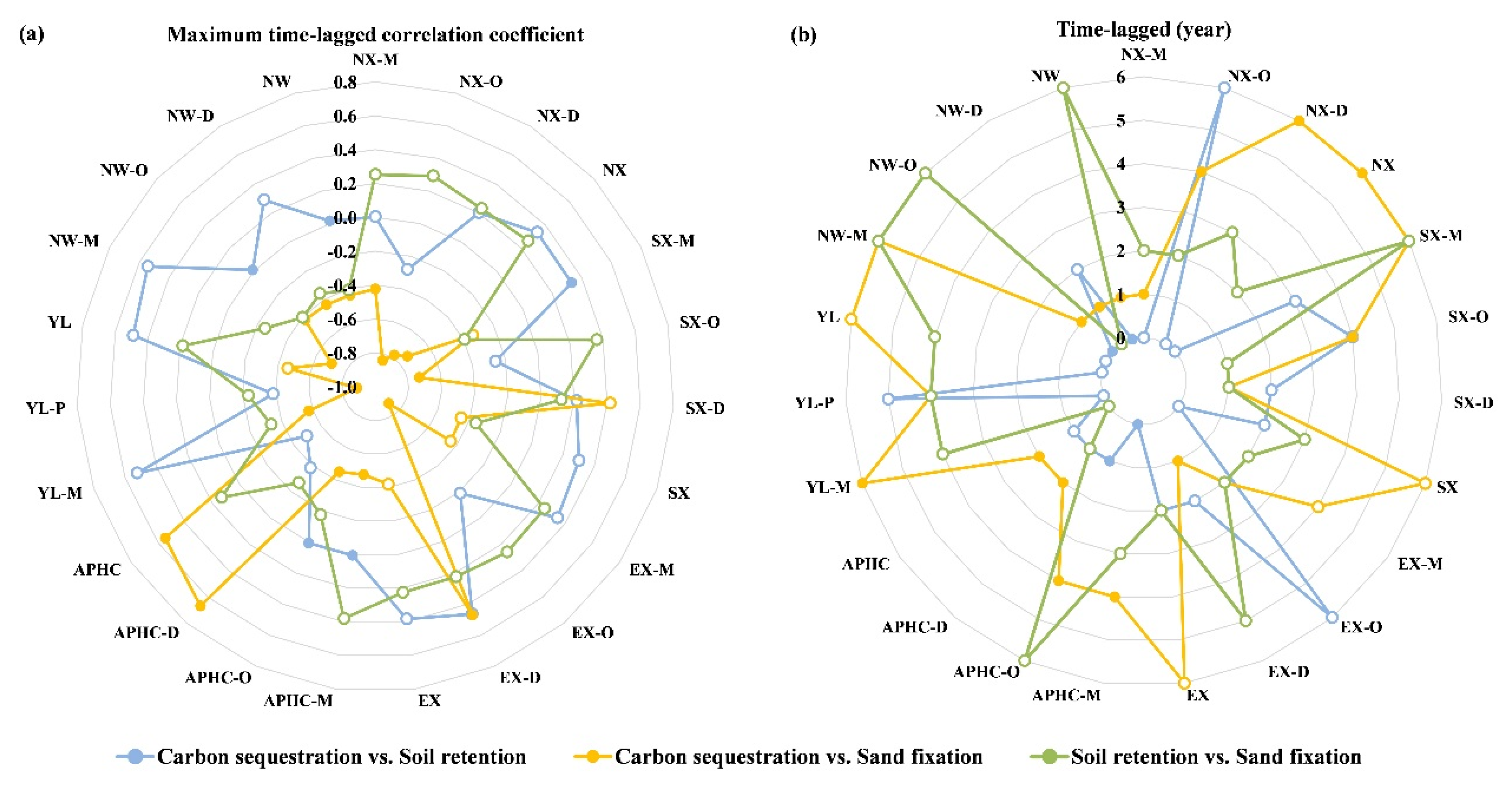
3.3. Time-Lagged Correlation of ESs Pairs

The corresponding correlation coefficients of carbon sequestration, soil retention, and sand fixation at each time-lag were calculated based on the principle of the time-lagged cross-correlation method. Then, the maximum time-lagged correlation coefficients were selected based on their significant linear relationships (p < 0.05), and their corresponding time-lags were regarded as the interaction time range among them. These results are illustrated by the radar charts (Figure 5). According to the study of Li Boyan et al. [17], the time trade-off is the maximum time-lagged correlation coefficient that is significant and less than 0, and its corresponding time is the trade-off time; the time synergy is the maximum time-lagged correlation coefficient that is significant and greater than 0, and its corresponding time is synergistic time.

The maximum correlation coefficients of carbon sequestration and sand fixation had obvious regional differences (Figure 5a), and most regions (i.e., 18 out of 23 regions) passed a significance test among various spatial scales. Here, all oasis sub-regions, including the plains of YL and NW-O, had significant time trade-offs. Half of the mountainous sub-regions had a significant time trade-off like the mountains across the whole NW. Two out of the four desert sub-regions with significant relationships had time trade-offs, while the other two had time synergies. These differences among the oases themselves, among the mountains themselves, and among deserts themselves seem not to influence the time-lagged correlation between the carbon sequestration and sand fixation of MODS at the spatial scale of the whole NW, and they all presented time trade-offs with the maximum time-lagged correlation coefficients of −0.704, −0.422, and −0.434, respectively. Correspondingly, the time-lag of the oases ranged from 1–4 years (Figure 5b), and half of them were delayed by four years. All oasis sub-regions had longer time-lags than the oases for the whole NW (i.e., one year), which means that the time-lag of the whole NW does not equal or approximate the average of the values of all its components. For the mountainous sub-regions and desert sub-regions, the time-lag was mainly concentrated at the one year, four year, and six year time ranges, and at the one year, two year, and six year time ranges, respectively.

A few of the regional maximum correlation coefficients between carbon sequestration and soil retention passed the given significance level, including NX-M (0.004), APHC-M (0.005), APHC-O (0.007), NW-O (0.010), and NW (0.017) (Figure 5a). All these coefficients showed weak time synergies due to their values being much less than 1. The relationships among mountains and among oases displayed great spatial differences, and there were few significant interactions in the mountains (i.e., 2 out of 6 mountainous sub-regions), few significances in the oases (i.e., 1 out of 5 oasis sub-regions), and no significant relationship in the deserts. However, based on the scale of the whole NW, both NW-O and the whole NW had significant time synergies. Moreover, only APHC-O had a 1-year time lag among these significant time synergy regions (Figure 5b). There was no significant difference among all regional maximum correlation coefficients between soil retention and sand fixation, regardless of the sub-regions, parts, or MODS of the whole arid area (Figure 5a).

4. Discussion

4.1. Explanation of the Interactions between ESs

The spatial scale was not only reflected by the trend of each ES but also by relationships among ESs. At the sub-regional scale, most relationships among ESs in the MODS of the whole NW were not consistent with those in the MODS of each large region; this difference varied over time and space. For example, during 1990–2015, trade-offs between carbon sequestration and soil retention were found for the oases and deserts of the APHC and the mountains of the APHC with synergy, but synergies occurred at the MODS for the whole NW. Therefore, interactions between ESs at microscopic scales may be hidden at the macroscopic scale. Although synergies between carbon sequestration and soil retention occurred in most areas of the NW and during most periods, continuous trade-offs happened in APHC-O and EX-O. These conflicting relationships between carbon sequestration and soil retention could be explained by the constraint threshold theory, proposed by Hao Ruifang et al. [31], where this relationship is characterized by a hump-shaped line. Higher carbon sequestration indicates good vegetation coverage that could protect soil from erosion by water or indicates more precipitation, which could increase the possibility of soil erosion. These multiple factors may jointly affect the relationship of carbon sequestration and soil retention. During 1990–2015, the carbon sequestration of APHC-O and EX-O exceeded the constraint threshold, which restricted the improvement of soil retention [20]. Meanwhile, the relationship among multiple ecosystem services reveals some degree of evolution, and this development is multistage and distinct [32,33]. For example, the relationship between carbon sequestration and soil retention in NX-D converted from a trade-off to synergy relationship. Carbon sequestration with the other two ESs both have time-lags; these delayed effects may result from the changes of vegetation coverage in the study area, based on the historical influence of land use/cover on the current provisions of ESs [13,34]. Further, a greater absolute value of the maximum time-lagged correlation coefficient corresponded to a longer time-lag.

4.2. Implications of Ecosystem Services Assessment for Ecological Management

The carbon sequestration of the most arid area has improved over the past 26 years and has shifted in the mountains and deserts around the year 2000. The Tianshan Mountains–Altai Mountains Natural Forest Protection Project launched in 2000, effectively protecting state-owned natural forests by expanding ecological forest land based on rational zoning, changing the business direction of forest industry enterprises to silvicultural treatments, and reducing the timber output [35]. Carbon sequestration of the whole arid area changed around 2000, possibly because of the increase in biological sand barriers to combat sand movement in the deserts of APHC. Although the protection of desert Populus diversifolia was strengthened in 1980, most areas of the protected region were relatively small, such as gardens or belts alongshore rivers or lakes. However, the declining carbon sequestration of desert eco-regions needs to be paid more attention to, particularly EX-O and SX-O. Carbon sequestration reflects vegetation density and growth conditions, and vegetation coverage has degraded severely across these two regions [20]. Therefore, the key to increasing the ability of carbon sequestration is an improvement of vegetation coverage. Increasing the amount of water availability (e.g., precipitation, evapotranspiration, soil wetness, and humidity) is a widely accepted and recommended approach [20,36]. Due to a deficiency in natural water, eco-environment water (3.6%) is used by agricultural irrigation (about 92%–95%) [37]. Breeding native plant species (e.g., Eurotia arborescens ALos, Caragana Korshinsii Kom, Psammochloa mongolica, and Calligunum mongolicum Turcz) and applying drip irrigation technology may improve this degeneration of future ecosystem management. Due to the declined provision of soil retention and the warming climate in the NW [38], more runoff has been yielded by melting high-altitude glaciers (e.g., the Tian Shan in the Xinjiang) and snow water flows to the plains or basins [39]; this process can remove soil and its fertilizer. In addition, increasing the area of farmland results in greater damage to the soil’s surface after tillage. Wind-break and sand-fixation efforts in the APHC in the 1990s, may have caused an increase of sand fixation in the APHC, which was mainly supported by the implementation of the Gansu Integrated Desert Control and Sustainable Agriculture Project [40]. This project combined physical sand-fixation technologies (e.g., straw checkerboard barriers and an enclosure zone for natural vegetation) and biological technologies (e.g., a farmland shelterbelt net and a vegetation arrangement for windbreak). To encourage people to positively participate in ecological work, the plants selected as vegetation to prevent land desertification could include drought-enduring medicinal herbs with excellent self-survival or grass for forage. The considerable economic benefits of these plants could stimulate participants to continue the work. As one of the sources of sandstorms, the arid area of northwestern China carries sand and greatly impacts the sandstorm frequency downwind of Beijing and Tianjin, but the Badain Jaran Desert (i.e., the desert to the west of the Alxa desert, Inner Mongolia) was not covered by the second round of the improvement project of the Beijing–Tianjin sandstorm source region [41]. In the future, plans for this arid area may improve the effectiveness of controlling sandstorm projects. For the whole northwest arid area, availability water and existing vegetation are both important for the ecological environment. Therefore, the punishments for damaging natural forests and polluting water could be increased in severity. Meanwhile, raising the price of agricultural water could restrict water-wasting behaviors. Ecological recovery and reconstruction need to be optimized stepwise, along with problem diagnoses, planning, implementation, monitoring, and evaluation [42]. Considering the dynamic nature of the ecosystem’s components, structure, progress, and functions, the evolution of the ecosystem and landscape present various uncertainties in ecological recovery applications, even those under artificial control. The costs of each plan, and their participants, also influence the implementation of ecological projects. Our results only offer some preliminary suggestions from the perspective of ecosystem services. The dynamic and continuous multi-aspect (e.g., investment and costs, willingness of participants, and ecosystem quality) activities of supervision, analysis, and assessment should be further enhanced.

4.3. Limitations and Improvements Methods

We recognize some limitations of this study. The first lies in the linear correlation analysis of the relationship among ESs, which assumes that the relationships between ecosystem services are monotonic. However, considering the complexity and diversity of the ecosystem process, there may be more types of interactions among them, such as constraint effects with diverse shapes [31], as well as trade-offs and synergistic relationships depicted by a bagplot [43]. Therefore, it is necessary to adopt some nonlinear statistical analyses (e.g., a segmented linear regression, an accumulative probability density curve, and logarithmic function fitness) to explore these relationships. The second limitation is that the effects of spatial scale have been shown in the current research, but a finer spatial scale would allow land-use policy-makers and ecological planners to acquire more explicitly spatial information. In future research, ESs and their relationships with the others, as well as their associations with potential contributors (like climate change and anthropic activities), could be assessed at a grid-cell scale. Moreover, more detailed ecological levels (like ecosystem class and landscape level) could be evaluated to enrich our understanding of ESs. The third limitation is that errors in the regionalization of MODS may influence determinations of the relationship type between pair-wised ESs. On-the-spot investigations could be conducive to reducing error and may help further reveal the regular patterns in different eco-regions. Last but not least, there are problems in the validations of the ESs estimated by the biophysical progress model; these difficulties result from the lack of observations in the study regions and the inconsistencies between observations and scaled extrapolation results. This is an important and challenging matter for ES assessment.

5. Conclusions

In summary, our study provided a quantitative assessment of the dynamics of ecosystem services (i.e., carbon sequestration, soil retention, and sand fixation) and their interrelationships over space and time in the arid area of northwestern China. We found that the ecosystem services of most of the arid area declined. Carbon sequestration in the oases continued to increase, and sand fixation of the Alxa Plateau–Hexi Corridor area, before 2000, improved markedly due to the great efforts of wind-break and sand-fixation. The trade-offs between carbon sequestration and soil retention mostly affected all periods and all sub-regions. The time-lagged trade-offs between carbon sequestration and sand fixation occurred widely in the arid area, and a greater maximum correlation coefficient resulted in a longer time-lag. These results highlight that interactions between ecosystem services vary over temporal and spatial scales. The enhancement of carbon sequestration in deserts and soil retention and sand fixation in most arid areas could be future targets for ecological restoration.

References

1. Costanza, R.; dArge, R.; deGroot, R.; Farber, S.; Grasso, M.; Hannon, B.; Limburg, K.; Naeem, S.; Oneill, R.V.; Paruelo, J.; et al. The value of the world’s ecosystem services and natural capital. Nature 1997, 387, 253–260. [Google Scholar] [CrossRef]
2. Millennium Ecosystem Assessment. Ecosystems and Human Well-Being: Synthesis; Island Press: Washington DC, USA, 2005. [Google Scholar]
3. Costanza, R.; de Groot, R.; Braat, L.; Kubiszewski, I.; Fioramonti, L.; Sutton, P.; Farber, S.; Grasso, M. Twenty years of ecosystem services: How far have we come and how far do we still need to go? Ecosyst. Serv. 2017, 28, 1–16. [Google Scholar] [CrossRef]
4. Xie, G.D.; Lu, C.; Leng, Y.; Zhang, D.; Li, S. Ecological assets valuation of the Tibetan Plateau. J. Nat. Resour. 2003, 18, 189–196. [Google Scholar]
5. Ling, H.B.; Yan, J.J.; Xu, H.L.; Guo, B.; Zhang, Q.Q. Estimates of shifts in ecosystem service values due to changes in key factors in the Manas River basin, northwest China. Sci. Total Environ. 2019, 659, 177–187. [Google Scholar] [CrossRef]
6. Xie, G.D.; Zhang, C.X.; Zhang, L.M.; Chen, W.H.; Li, S.M. Improvement of the evaluation method for ecosystem service value based on per unit area. J. Nat. Resour. 2015, 30, 1243–1254. [Google Scholar]
7. Barral, M.P.; Oscar, M.N. Land-use planning based on ecosystem service assessment: A case study in the Southeast Pampas of Argentina. Agric. Ecostst. Environ. 2012, 154, 34–43. [Google Scholar] [CrossRef]
8. Carreno, L.; Frank, F.C.; Viglizzo, E.F. Tradeoffs between economic and ecosystem services in Argentina during 50 years of land-use change. Agric. Ecosyst. Environ. 2012, 154, 68–77. [Google Scholar] [CrossRef]
9. Zhang, L.W.; Lu, Y.H.; Fu, B.J.; Dong, Z.B.; Zeng, Y.; Wu, B.F. Mapping ecosystem services for China’s ecoregions with a biophysical surrogate approach. Landsc. Urban Plan. 2017, 161, 22–31. [Google Scholar] [CrossRef]
10. Xu, Z.H.; Fan, W.G.; Wei, H.J.; Zhang, P.; Ren, J.H.; Gao, Z.C.; Ulgiati, S.; Kong, W.D.; Dong, X.B. Evaluation and simulation of the impact of land use change on ecosystem services based on a carbon flow model: A case study of the Manas River Basin of Xinjiang, China. Sci. Total Environ. 2019, 652, 117–133. [Google Scholar] [CrossRef]
11. Zhang, H.Y.; Fan, J.W.; Cao, W.; Harris, W.; Li, Y.Z.; Chi, W.F.; Wang, S.Z. Response of wind erosion dynamics to climate change and human activity in Inner Mongolia, China during 1990 to 2015. Sci. Total Environ. 2018, 639, 1038–1050. [Google Scholar] [CrossRef]
12. Jiang, C.; Nath, R.; Labzovskii, L.; Wang, D.W. Integrating ecosystem services into effectiveness assessment of ecological restoration program in northern China’s arid areas: Insights from the Beijing-Tianjin Sandstorm Source Region. Land Use Pol. 2018, 75, 201–214. [Google Scholar] [CrossRef]
13. Jiang, C.; Liu, J.G.; Zhang, H.Y.; Zhang, Z.D.; Wang, D.W. China’s progress towards sustainable land degradation control: Insights from the northwest arid regions. Ecol. Eng. 2019, 127, 75–87. [Google Scholar] [CrossRef]
14. Ouyang, Z.Y.; Zheng, H.; Xiao, Y.; Polasky, S.; Liu, J.; Xu, W.; Wang, Q.; Zhang, L.; Xiao, Y.; Rao, E.M.; et al. Improvements in ecosystem services from investments in natural capital. Science 2016, 352, 1455–1459. [Google Scholar] [CrossRef] [PubMed]
15. Xu, S.; Liu, Y.F. Associations among ecosystem services from local perspectives. Sci. Total Environ. 2019, 690, 790–798. [Google Scholar] [CrossRef] [PubMed]
16. Hou, Y.; Lu, Y.H.; Chen, W.P.; Fu, B.J. Temporal variation and spatial scale dependency of ecosystem service interactions: A case study on the central Loess Plateau of China. Landsc. Ecol. 2017, 32, 1201–1217. [Google Scholar] [CrossRef]
17. Li, B.Y.; Chen, N.C.; Wang, Y.C.; Wang, W. Spatio-temporal quantification of the trade-offs and synergies among ecosystem services based on grid-cells: A case study of Guanzhong Basin, NW China. Ecol. Indic. 2018, 94, 246–253. [Google Scholar] [CrossRef]
18. Daily, G.C.; Polasky, S.; Goldstein, J.; Kareiva, P.M.; Mooney, H.A.; Pejchar, L.; Ricketts, T.H.; Salzman, J.; Shallenberger, R. Ecosystem services in decision making: Time to deliver. Front. Ecol. Environ. 2009, 7, 21–28. [Google Scholar] [CrossRef] [Green Version]
19. Zagonari, F. Using ecosystem services in decision-making to support sustainable development: Critiques, model development, a case study, and perspectives. Sci. Total Environ. 2016, 548, 25–32. [Google Scholar] [CrossRef]
20. Liu, Y.; Li, L.H.; Chen, X.; Zhang, R.; Yang, J.M. Temporal-spatial variations and influencing factors of vegetation cover in Xinjiang from 1982 to 2013 based on GIMMS-NDVI3g. Glob. Planet. Chang. 2018, 169, 145–155. [Google Scholar] [CrossRef]
21. Jiapaer, G.; Liang, S.L.; Yi, Q.X.; Liu, J.P. Vegetation dynamics and responses to recent climate change in Xinjiang using leaf area index as an indicator. Ecol. Indic. 2015, 58, 64–76. [Google Scholar] [CrossRef]
22. Wang, Z.; Shi, Q.S.; Wang, T.; Shi, Q.D.; Chang, S.L.; Zhang, L.B. Spatial-temporal characteristics of vegetation cover change in mountain-oasis-desert system of Xinjiang from 1982 to 2006. J. Nat. Resour. 2011, 26, 609–618. [Google Scholar]
23. Potter, C.S.; Randerson, J.T.; Field, C.B.; Matson, P.A.; Vitousek, P.M.; Mooney, H.A.; Klooster, S.A. Terrestrial ecosystem production -a process model-based on global satellite and surface data. Glob. Biogeochem. Cycle 1993, 7, 811–841. [Google Scholar] [CrossRef]
24. Xiao, X.M.; Zhang, Q.Y.; Braswell, B.; Urbanski, S.; Boles, S.; Wofsy, S.; Berrien, M.; Ojima, D. Modeling gross primary production of temperate deciduous broadleaf forest using satellite images and climate data. Remote Sens. Environ. 2004, 91, 256–270. [Google Scholar] [CrossRef]
25. Ryu, Y.; Baldocchi, D.D.; Black, T.A.; Detto, M.; Law, B.E.; Leuning, R.; Miyata, A.; Reichstein, M.; Vargas, R.; Ammann, C.; et al. On the temporal upscaling of evapotranspiration from instantaneous remote sensing measurements to 8-day mean daily-sums. Agric. For. Meteorol. 2012, 152, 212–222. [Google Scholar] [CrossRef] [Green Version]
26. Wang, J.B.; Liu, J.Y.; Shao, Q.Q.; Liu, R.G.; Fan, J.W.; Chen, Z.Q. Spatial-temoral patterns of net primary productivity for 1988–2004 based on GLOPEM-CEVSA model in the Three-River Headwaters region of Qianghai Province, China. Acta Phytoecol. Sin. 2009, 33, 254–269. [Google Scholar]
27. Jiao, W.; Chen, Y.N.; Li, W.H.; Zhu, C.G.; Li, Z. Estimation of net primary productivity and its driving factors in the Ili River Valley, China. J. Arid Land 2018, 10, 781–793. [Google Scholar] [CrossRef] [Green Version]
28. Zhu, W.Q.; Pan, Y.Z.; Zhang, J.S. Estimation of net primary productivity of Chinese terrestrial vegetation based on remote sensing. J. Plant Ecol. 2007, 31, 413–424. [Google Scholar]
29. Yang, F.B.; Lu, C.H. Spatiotemporal variation and trends in rainfall erosivity in China’s dryland region during 1961–2012. Catena 2015, 133, 362–372. [Google Scholar] [CrossRef]
30. Fryrear, D.; Saleh, A.; Bilbro, J.; Shomberg, H.; Stout, J.; Zobeck, T. Revised Wind Erosion Equation (RWEQ). Wind Erosion and Water Conservation Research Unit, USDA-ARS, Southern Plains Area Cropping Systems Research Laboratory. Tech. Bull. 1998, 1. [Google Scholar]
31. Hao, R.F.; Yu, D.Y.; Wu, J.G. Relationship between paired ecosystem services in the grassland and agro-pastoral transitional zone of China using the constraint line method. Agric. Ecostst. Environ. 2017, 240, 171–181. [Google Scholar] [CrossRef]
32. Renard, D.; Rhemtulla, J.M.; Bennett, E.M. Historical dynamics in ecosystem service bundles. Proc. Natl. Acad. Sci. USA 2015, 112, 13411–13416. [Google Scholar] [CrossRef] [PubMed] [Green Version]
33. Wu, J.X.; Zhao, Y.; Yu, C.; Luo, L.; Pan, Y. Land management influences trade-offs and the total supply of ecosystem services in alpine grassland in Tibet, China. J. Environ. Manag. 2017, 193, 70–78. [Google Scholar] [CrossRef] [PubMed]
34. Dallimer, M.; Davies, Z.G.; Diaz-Porras, D.F.; Irvine, K.N.; Maltby, L.; Warren, P.H.; Armsworth, P.R.; Gaston, K.J. Historical influences on the current provision of multiple ecosystem services. Glob. Environ. Chang. Hum. Policy Dimens. 2015, 31, 307–317. [Google Scholar] [CrossRef] [Green Version]
35. Sun, H.L.; Zhao, S.D. Area Studies (Regional Sustainable Development Review): China-Volume I; EOLSS Publications: Oxford, UK, 2009; pp. 122–123. [Google Scholar]
36. Nemani, R.R.; Keeling, C.D.; Hashimoto, H.; Jolly, W.M.; Piper, S.C.; Tucker, C.J.; Myneni, R.B.; Running, S.W. Climate-driven increases in global terrestrial net primary production from 1982 to 1999. Science 2003, 300, 1560–1563. [Google Scholar] [CrossRef] [Green Version]
37. Guan, Y.; He, Z.L.; Zhang, B.; Li, L. Analysis on current situation rationality of development and utilization of water resources in Xinjiang Wei Autonomous Region. Bull. Soil Water Conserv. 2006, 26, 104–106. [Google Scholar]
38. Yao, J.Q.; Zhao, Y.; Chen, Y.N.; Yu, X.J.; Zhang, R.B. Multi-scale assessments of droughts: A case study in Xinjiang, China. Sci. Total Environ. 2018, 630, 444–452. [Google Scholar] [CrossRef]
39. Yao, J.Q.; Hu, W.F.; Chen, Y.N.; Huo, W.; Zhao, Y.; Mao, W.Y.; Yang, Q. Hydro-climatic changes and their impacts on vegetation in Xinjiang, Central Asia. Sci. Total Environ. 2019, 660, 724–732. [Google Scholar] [CrossRef]
40. Xu, X.Y. Restrospect and prospect of 60-year sand conctol research in Gansu province. For. Gansu Prov. 2019, 4, 9–21. [Google Scholar]
41. Research Project Group for the Second Phase of the Beijing-Tianjin Sandstorm Source Control Project. Research on the Second Phase Planning of Beijing-Tianjin Sandstorm Source Control Project; China Forestry Publishing House: Beijing, China, 2013. [Google Scholar]
42. Lv, Y.H.; Fu, B.J.; Chen, L.D. Ecological rehabilitation: A theoretical analysis. Acta Ecol. Sin. 2006, 26, 3891–3897. [Google Scholar]
43. Jopke, C.; Kreyling, J.; Maes, J.; Koellner, T. Interactions among ecosystem services across Europe: Bagplots and cumulative correlation coefficients reveal synergies, trade-offs, and regional patterns. Ecol. Indic. 2015, 49, 46–52. [Google Scholar] [CrossRef]
Figure 1. Spatial pattern of the mountain–oasis–desert system (MODS). Large parts and MODS sub-regions are separated by short dashes. M: mountains; O: oasis; D: deserts; P: plains.
Sustainability 12 00803 g001
Figure 2. Spatial distribution of the three ESs over the whole northwestern arid area. (a) Annual average carbon sequestration, (b) annual average soil retention, (c) annual average sand fixation.
Sustainability 12 00803 g002
Figure 3. Temporal change trends of the ESs during the three periods (i.e., before 2000, after 2000, and 1990–2015) for the MODS of the northwestern arid area. (a1a3) Carbon sequestration, (b1b3) soil retention, and (c1c3) sand fixation.
Sustainability 12 00803 g003
Figure 4. Trade-offs and synergies of ecosystem service pairs. (a) Carbon sequestration vs. soil retention, (b) Carbon sequestration vs. sand fixation, (c) sand fixation vs. soil retention.
Sustainability 12 00803 g004
Figure 5. The maximum correlation coefficient and lag time of pair-wise ESs in the northwestern arid area. (a) The maximum time-lagged correlation coefficients between carbon sequestration and soil retention, carbon sequestration and sand fixation, and soil retention and sand fixation. (b) The time-lags corresponding to the maximum time-lagged correlation coefficients between carbon sequestration and soil retention, carbon sequestration and sand fixation, and soil retention and sand fixation; (a) and (b) the five large parts, 14 sub-regions, and MODS of the whole arid area. Solid circles represent estimates that passed a significance of p < 0.05, and the circles represent insignificance.
Sustainability 12 00803 g005