Identification of Heracleum sosnowskyi-Invaded Land Using Earth Remote Sensing Data


1
Department of Geodesy and Cadastre, Vilnius Gediminas Technical University, Sauletekio av. 11, LT-10223 Vilnius, Lithuania
2
Institute of Land Management and Geomatics, Vytautas Magnus University Agriculture Academy, Studentu 11, Akademija, LT-53361 Kaunas district, Lithuania
3
Department of the Built Environment, Built Environment and Sustainable Technologies Research Institute, Faculty of Engineering and Technology, Liverpool John Moores University, Byrom street, Liverpool L3 3AF, UK
*
Authors to whom correspondence should be addressed.
Sustainability 2020, 12(3), 759; https://doi.org/10.3390/su12030759
Submission received: 5 December 2019
/
Revised: 9 January 2020
/
Accepted: 19 January 2020
/
Published: 21 January 2020
(This article belongs to the Special Issue Land and Water Degradation in Catchments: The Role of Remote Sensing for Assessment and Management)
Abstract
:H. sosnowskyi (Heracleum sosnowskyi) is a plant that is widespread both in Lithuania and other countries and causes abundant problems. The damage caused by the population of the plant is many-sided: it menaces the biodiversity of the land, poses risk to human health, and causes considerable economic losses. In order to find effective and complex measures against this invasive plant, it is very important to identify places and areas where H. sosnowskyi grows, carry out a detailed analysis, and monitor its spread to avoid leaving this process to chance. In this paper, the remote sensing methodology was proposed to identify territories covered with H. sosnowskyi plants (land classification). Two categories of land cover classification were used: supervised (human-guided) and unsupervised (calculated by software). In the application of the supervised method, the average wavelength of the spectrum of H. sosnowskyi was calculated for the classification of the RGB image and according to this, the unsupervised classification by the program was accomplished. The combination of both classification methods, performed in steps, allowed obtaining better results than using one. The application of authors’ proposed methodology was demonstrated in a Lithuanian case study discussed in this paper.
1. Introduction
Invasive plants have turned into a global intractable problem both in Lithuania and other states. One such plant is Heracleum sosnowskyi (H. sosnowskyi). In addition to being a menace to the biodiversity of the land, wide spread of said plant causes considerable economic losses and poses a risk to human health because the plant provokes the appearance of long-lasting burns on the skin. The H. sosnowskyi is an invasive alien species from the Caucasus. It is a biennial or a perennial plant. Its height is usually 100–300 cm. Flowering typically lasts from June to August [1]. Several botanists consider H. sosnowskyi only as the subtaxon of Heracleum mantegazzianum or Hypericum pubescens. Therefore, H. sosnowskyi does not appear in the lists of weedy flora of many Western European countries. It was described as a separate species by I. Mandenova in 1944 [2].
H. sosnowskyi was brought to Lithuania, as well as to Estonia, Latvia, Belarus, Ukraine, Poland, and Germany, about 1944–1950 and in the beginning was cultivated as a fodder plant.
In the Soviet period, some people started cultivating H. sosnowskyi as an ornamental plant in their gardens because of its impressive appearance and large inflorescence. For a long time, apiarists were sure that bees collected nectar from H. sosnowskyi. In 1958, Wroclaw Medical Academy (Poland) sowed H. sosnowskyi as a medicinal plant [3]. However, when signs of its spread were detected, doubts about the benefit of this plant appeared because H. sosnowskyi was found in fields of 17 districts of Lithuania before the year 1990 and by about 2005, it had already spread almost everywhere over Lithuania. In large inflorescences, each plant nurtures tens of thousands of seeds annually (the largest plants–even up to 100,000 seeds), interspersing them within the radius of about 4 meters, so they spread very rapidly. Up to 95% of the seeds remain viable for several years. In addition, this plant is difficult to eradicate because it regrows from its roots even after several cuttings out.
Investigations of plant communities with H. sosnowskyi were performed in 2002–2004 all over Lithuania [4]. Therefore, Z. Gudžinskas and E. Žalneravičius studied the seeding dynamics and the population structure in Lithuania. These results are important from a theoretical point of view and can also be helpful in selection of effective measures for management and eradication of H. sosnowskyi [5]. In Lithuania, H. sosnowskyi was included in the list of plants harmful for human health that should be eradicated [6,7]. Three meters high H. sosnowskyi (and even higher) choke growing of a majority of local plants. In the localities where H. sosnowskyi appears once, it soon becomes a predominating plant. The causes of rapid spread, invasiveness, and environmental hazardousness of H. sosnowskyi and other large hogweeds are bound with the biological and ecological properties of the plant. Changes of the landscape caused by the high plants are extremely negative [8]. Data indicate that the invasive species of the genus Heracleum can be a serious threat to people living next to them due to their toxicity [9]. In Lithuania, H. sosnowskyi usually grows in grasslands, outskirts, and various areas of anthropogenic origin of various types (such as waysides, wastelands, abandoned farmlands, quarries, and so on), and grows more rarely in forest and shrub communities (tree strata of various compositions and ages). As early as in 2000–2005, it was found from the data of the survey research that H. sosnowskyi overgrowths of different sizes and densities cover about 10’000 ha in Lithuania. About 80% of the area is formed by H. sosnowskyi growing within cultivated grasslands and pastures, abandoned farmlands, former outhouses, roadsides, at farmyards, and so on [8].
In 2016, this plant was recognized as an invasive plant in the European Union too. So, the European Commission initiated the EMPHASIS project (Effective Management of Pests and Harmful Alien Species –Integrated Solutions). One of the goals of the project is to find more effective measures for the eradication of H. sosnowskyi.
Nevertheless, prior to applying complex methods in the struggle against this plant, it is very important to identify the places and areas where H. sosnowskyi grows, as well as to carry out an exhaustive analysis and monitoring of its spread. The place of growing of the plant is a very important factor in choosing methods and measures for the eradication of H. sosnowskyi. For example, spraying herbicides was found to be an effective method in the struggle against H. sosnowskyi; however, it is not applicable everywhere. If precise data on places of H. sosnowskyi are available, the most effective, economic, and environmentally friendly method for eradicating this plant may be chosen and applied in a complex way.
The scientists J. Mullerova, P. Pyšek, V. Jarošik, and J. Pergl were assessing the dynamics of the plant Heracleum mantegazzianum (which is similar to H. sosnowskyi) from images in the Slovakovsky les protected landscape area. They found that information about the population characteristics from aerial images was limited by the quality of the photographs; however, some robust patterns over the 40 years of invasion could be identified [10]. Therefore, not all countries have the aerial images from the long period. The technology of remote sensing offers a practical and economical means to study vegetation cover changes, especially over large areas. Due to the potential capacity for systematic observations at various scales, remote sensing technology extends possible data archives from the present time to over several decades back [11,12]. There are two basic processes involved in the remote sensing technology: data (space images) processing (photogrammetry stages) and analyses of results (GIS stages). The sensing system is classified to the optical (passive) and radar (active) sensors and has different imaging mechanisms. The active system uses the solar energy independent of atmospheric monitoring and has a better capability of sensing vegetation and soil attributes that are dependent on moisture content, thus having immense value in various applications [13].
The authors of this paper focused on the identification of the H. sosnowskyi plant from remote sensing sensors, adapted image processing methods, and carried out classification accuracy assessments.
2. Materials and Methods
2.1. Test Area and Datasets
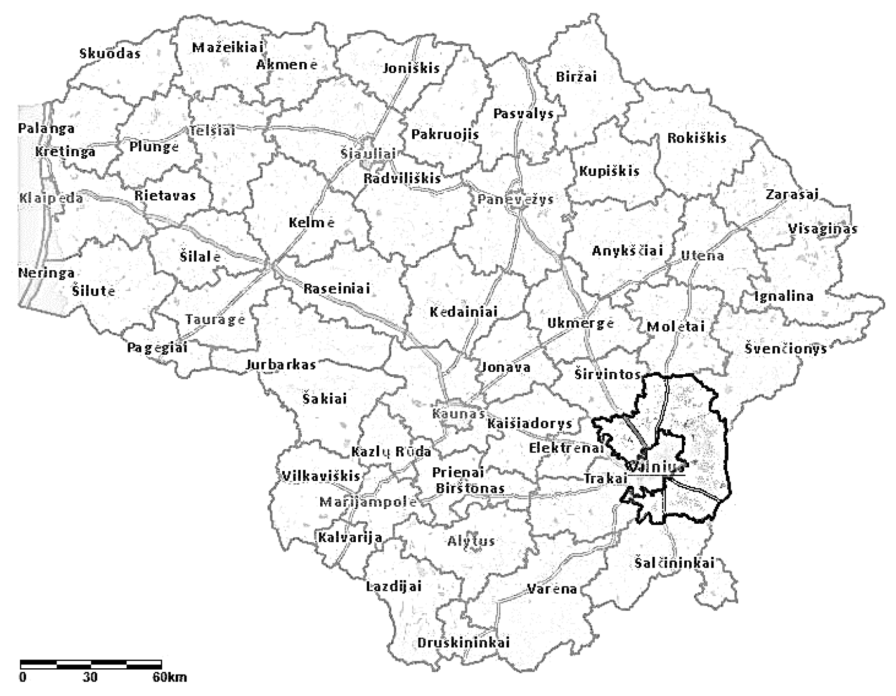
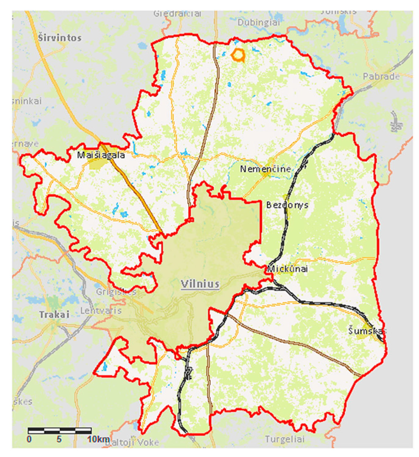
The selected research case study was Vilnius District Municipality, near Dirmeitai village (Figure 1 and Figure 2), as the majority of abandoned agricultural land, evaluating the total area of each municipality, was situated in Vilnius District Municipality [14].
In Lithuania, H. sosnowskyi usually grows namely on abandoned lands of agricultural purpose; in addition, it outspreads there and causes particularly extensive damage.
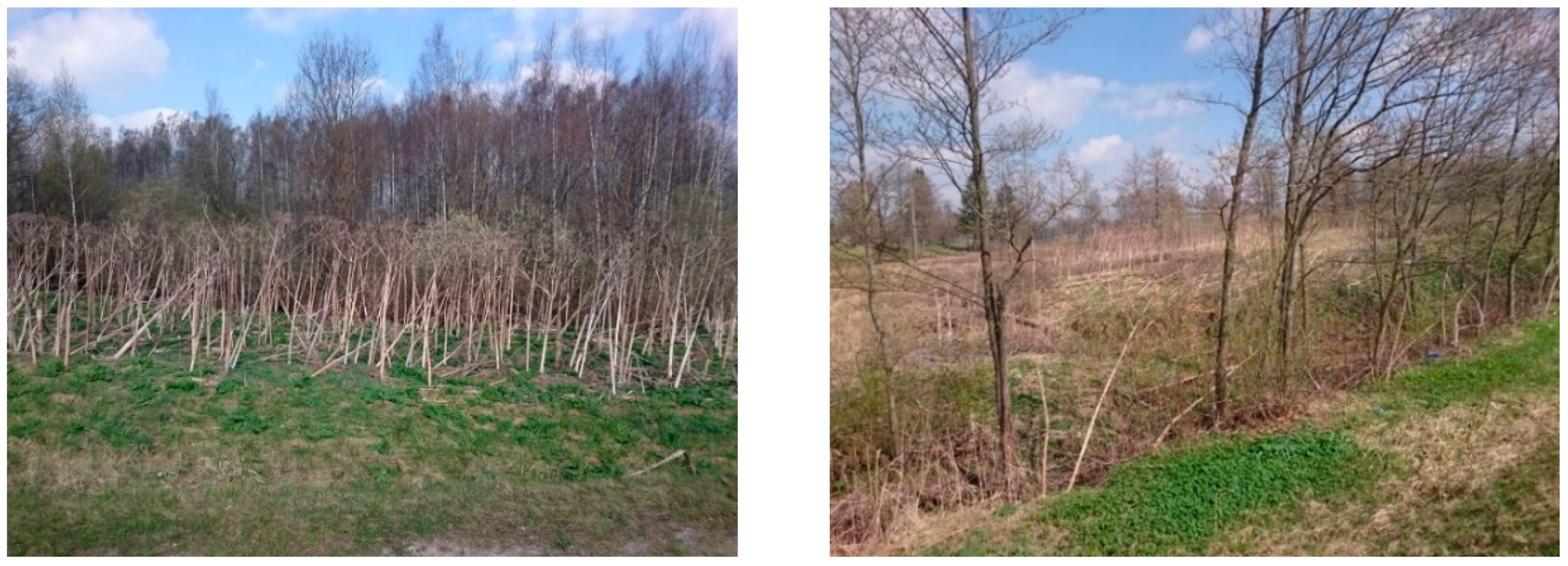
Prior to the investigation, the selected case study’s territory was inspected to make sure that H. sosnowskyi abundantly grows there. The real image of the territory near Dirmeitai village was fixed in April 2018 when the plants just began sprouting; however, the extant yesteryear stems were perfectly visible (Figure 3).
The remote sensing imaging is a key instrument that captures data about an object or scene remotely [4]. They can be identified from spectral features (reflectance or emission regions). Remote sensing imagery has a dependence on sensors with different wavelength (waveband) ranges. The different wavebands useful for hazard mapping and monitoring, also for land classification (land cover mapping), are shown in Table 1.
The MODIS near-infrared sensor from the Terra satellite is used for land imaging (Table 1) and provides high radiometric sensitivity (12 bit) in 36 spectral bands ranging in wavelength from 0.4 µm to 14.4 µm. Two bands are imaged at a nominal resolution of 250 m at nadir, with five bands at 500 m, and the remaining 29 bands at 1 km. A ±55° scanning pattern at the Earth Observing System (EOS) orbit of 705 km achieves a 2.330 km swath and provides global coverage every one to two days [17]. The AVHRR sensor image data have two spatial resolutions. They are 1.1 km for local area coverage and 5 km for global area coverage. In addition, imagery has a limitation in calibration. The Landsat Thematic Mapper (TM) and Enhanced Thematic Mapper (ETM) sensors provide medium spatial resolution images (30 m, 60 m) and are used for mapping at community level. All the mentioned sensors are not suitable for small areas. The Sentinel-1 SAR (synthetic aperture radar) mission supports land cover classification and change detection mapping. Sentinel-2’s MSI (multispectral instrument) support land monitoring services and provide spatial resolution (10 m, 20 m, 60 m) optical images. The Sentinel-3 IOLCI’s (International Ocean-Colour Coordinating Group, Canada) missions are maritime monitoring, land mapping and monitoring, atmospheric monitoring, and climate change monitoring. More information about Sentinel sensors is in the official ESA (Europe Space Agency, Netherlands) web site [18]. For the experimental part of the investigation, Sentinel satellite sensor data were applied. They were high-resolution optical images providing enhanced continuity of SPOT (French: Satellite Pour l’Observation de la Terre, English: Satellite for observation of Earth) and Landsat-type data [18]. Sentinel-2 carries an optical payload with visible, near infrared, and shortwave infrared sensors comprising 13 spectral bands: 4 bands at 10 m, 6 bands at 20 m, and 3 bands at 60 m spatial resolution (the latter is dedicated to atmospheric corrections and cloud screening), with a swath width of 290 km. The Sentinel data are available by the Copernicus Open Access Hub (COAH) Internet site [19] and orthoimage in the Lithuanian Spatial Information Portal: www.geoportal.lt. The case study territory (photographed in spring 2018, Figure 2 was analyzed using orthophoto images (scale 1:25,000). It was determined that the plant has a different green color brightness value in orthoimage, especially during the growing season. For the experiment, the Sentinel-2 space images data were downloaded on the following three dates: April, May, and October 2018. The images made in April 2018 was unsatisfactory due to the cloudiness at the time. The images made in May and October 2018 were of a satisfactory quality (Figure 4). The image Sentinel-2A, made in May 2018, was selected for the analysis. The Level-2A data included an atmospheric correction applied to top-of-atmosphere (TOA) Level-1C orthoimage products. Level-2A’s main output was an orthoimage bottom-of-atmosphere (BOA) corrected reflectance product [18].
The areas covered by H. sosnowskyi had a light green color in the Sentinel-2 image (Figure 4a,b). This exceptional fact encouraged us to carry out land cover classification processes for H. sosnowskyi identification. Multispectral images with true color composite RGB (red, green, and blue), at 10 and 20 m spatial resolution were used. The data were processed by software QGIS and eCognition.
2.2. Data Acquisition
The principle categories of deriving land cover from remotely sensed images are supervised (human-guided) or unsupervised (calculated by software) classification (or segmentation). The supervised classification can be automated or performed by manual interpretation. In the manual method, the operator is digitalizing the land cover boundaries upon using the GIS system, but these data are economically inefficient [20]. The scientists are still searching for new classification methods as traditional methods are very expensive [11]. The traditionally used clustering classification algorithms K-mean and ISODATA (iterative self-organizing data analysis technique A) involved iterative procedures by distance functions Di(x). The distance between pixels in feature space is the measure of similarity and is scaled in pixels, radiance, or reflectance. The relative distances may change when data are calibrated (digital counts ==> radiance), atmospherically corrected, or rescaled in ways that treat different spectral bands differently [20,21].
The K-mean is used to reduce the variability within the cluster. Many variations of the K-means algorithm have been developed, but the basic procedure steps are the following [21,22]:
1. Choose K initial cluster centers . Distribute the samples among the K-means. Samples should be assigned to the class represented by the nearest cluster center (Equation (1)):
where i ≠ j where is the set of samples whose cluster center is ; n indicates that this is the nth iteration of this procedure.
2. Compute new cluster centers for each set . Find a new value for each . The new cluster center (Equation (2)) will be the mean of all the points in such that:
3. Compare and for all i.
Compute the distance between each pair of points for the consecutive iterations.
The ISODATA algorithm is essentially a refinement of the K-Means algorithm. The specific refinements are [20]: clusters that have too few members are discarded; clusters that have too many members are split into two new cluster groups; clusters that are too large (too dispersed) are split into two new cluster groups; If two cluster centers are too close together then they are merged [20].
The cluster variability represents the mean square error of measurement (Equation (3)) [22]:
where D—distance between clusters; N—number of pixels; z—number of clusters; b—number of spectral bands in the image.
In the experiment, the region growing algorithm used by the authors allows for the selection of pixels similar to a seed one, considering the spectral similarity (spectral distance) of adjacent pixels [23]. Land covers are identified by the classes (Table 2). We selected class names—abundance land (ID1), H. sosnowskyi land (ID2), forest (ID3), etc. The spectral characteristics of reference land cover classes are calculated considering the values of pixels under each of the regions of interest (ROI) having the same class ID (or macro class ID). Therefore, the classification algorithm classifies the whole image by comparing the spectral characteristics of each pixel to the spectral characteristics of reference land cover classes [20]. The example shows the land cover signature classification for a simple case of two spectral bands x and y. The spectral regions define three classes (). The point p1 belongs to the class and point p2 belongs to the class . The point p3 is inside the spectral regions of both classes and (overlapping regions). The point p4 is outside any spectral region, therefore it will be unclassified or classified according to an additional classification algorithm.
- Minimum distance;
- Maximum likelihood;
- Spectral angle mapping.
The minimum distance algorithm calculates the Euclidean distance d(x,y) between spectral signatures of image pixels and training spectral signatures according to Equation (4) [20,23]:
here, x—spectral signature vector of an image pixel; y—spectral signature vector of a training area; n—number of image bands.
The distance is calculated for every pixel in the image, assigning the class of the spectral signature that is closer, according to the following discriminant function [20,24].
The maximum likelihood algorithm calculates the probability distributions for the classes, related to Bayes’ theorem, estimating whether a pixel belongs to a land cover class. In particular, the probability distributions for the classes are assumed the form of multivariate normal models [24]. In order to use this algorithm, a sufficient number of pixels is required for each training area, allowing for the calculation of the covariance matrix. The discriminant function, described by [24] (Equation (5)), is calculated for every pixel as:
where —land cover class k; x—spectral signature vector of a image pixel; —probability that the correct class is ; —determinant of the covariance matrix of the data in class ; Σk − 1—inverse of the covariance matrix; —spectral signature vector of class k.
The spectral angle mapping calculates the spectral angle between spectral signatures of image pixels and training spectral signatures. The spectral angle θ is defined as [25] (Equation (6)):
The spectral angle goes from 0 when signatures are identical to 90 when signatures are completely different [20].
In this paper, the authors combined these two categories of classification methods to identify the abundant land and H. sosnowskyi land cover in the RGB satellite image. The processing of RGB images was carried out using the open source QGIS 3.4.3-Madeira and commercial eCognition Essential 1.3 software. Four spectral bands with a spatial resolution of 10 m and 20 m were used to search for the plant in the H. sosnowskyi’s areas: blue B2 (447.6–545.6 nm), green B3 (537.5–582.5 nm), red B4 (645.5–683.5 nm), and near infrared (NIR) B8 (762.6–907.6 nm).
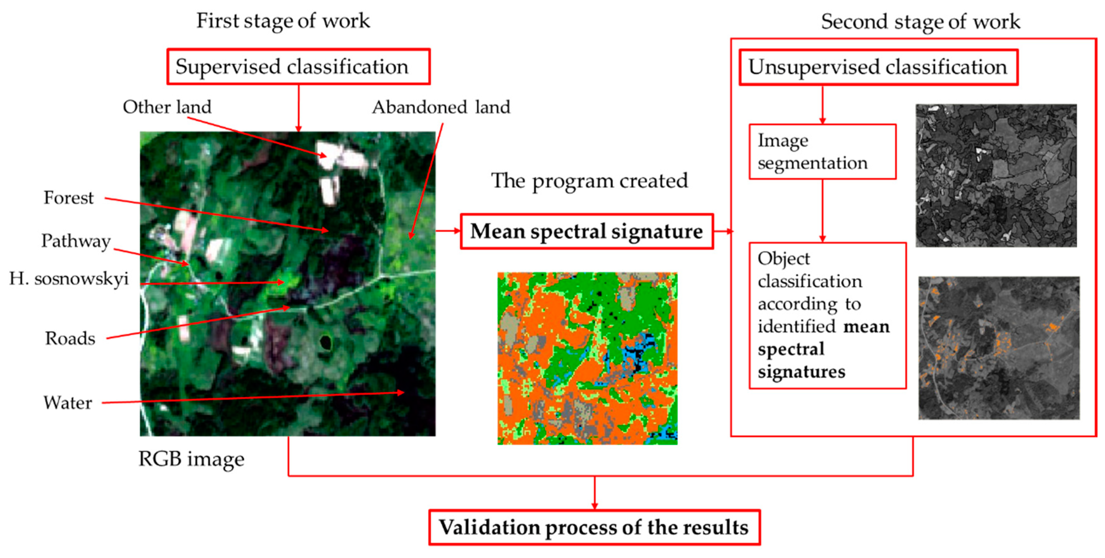
Two categories (supervised and unsupervised) of land cover classification were used for this study. The scheme of workflow is presented in the Figure 5.
3. Results and Discussion
The supervised classification goes through the following work steps: selection of training areas, generation of signature file, and classification of the features. Therefore, we have the mean spectral signature of land cover from all bands. In the first stages of the work, the authors were digitalizing the land cover boundaries using the GIS system (QGIS software). Land covers separately were identified at the spatial resolutions of 10 m and 20 m in a RGB image from May 2018. The selected classes included: abandoned land, forest, pathway, H. sosnowskyi, roads, water, and other land (used for agriculture land and building) (Table 2).
Results and statistics of classification of 10 m and 20 m RGB images are presented in Figure 6 and Figure 7.
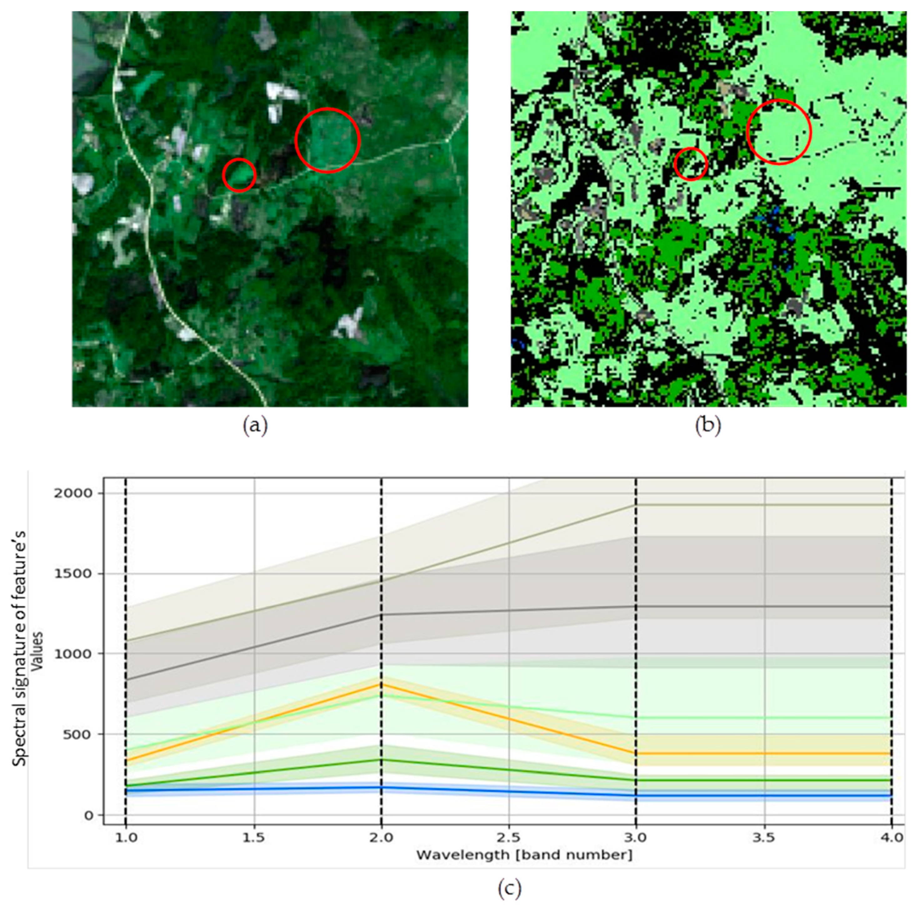
Results of classification in the 20 m RGB images show that the abandoned land class and H. sosnowskyi land class merge in to one feature spectral signature in Figure 7c. The authors of this paper took an interest in the mean spectral signature of abandoned land and H. sosnowskyi classes, so these land cover classes are highlighted in the summary of the statistical data (Table 3). In addition, important indicators (such as spectral angle, Euclidean distance, Bray–Curtis similarity) were calculated between the highlighted land cover classes and they show a similarity of the classification spectrum between plants (Table 4).
The feature classes established in this paper utilizing lands’ mean spectral signature differences allowed the authors to identify H. sosnowskyi land invasions (Table 2). In addition, the characteristics of the Bray–Curtis similarity between classes is high (90%). The results of different spatial resolutions of images have different mean spectral signatures.
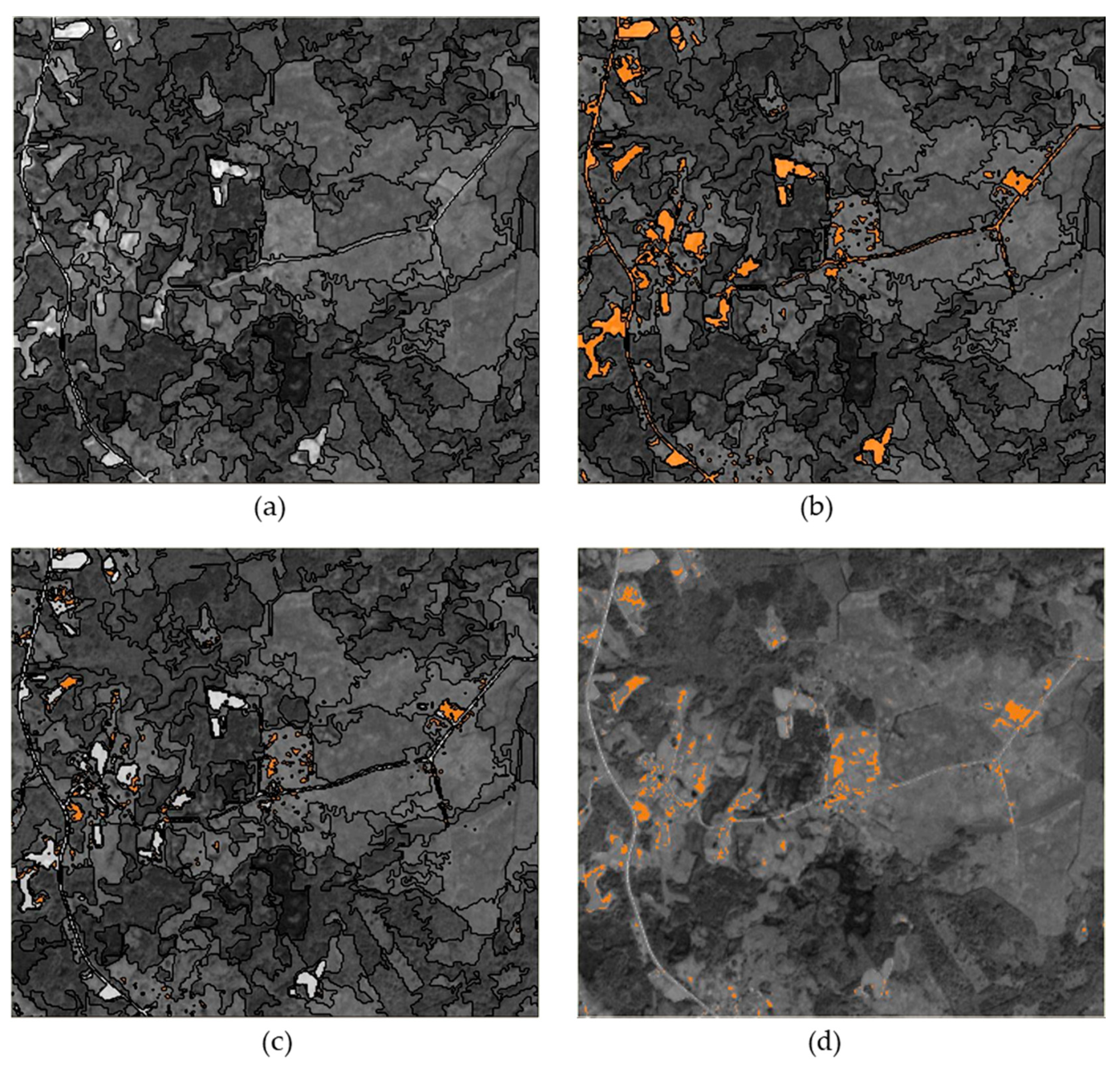
Therefore, the RGB image 10 m spatial resolution (Band 3 (Green)) result—the H. sosnowskyi mean spectral signature value 845.90 (Table 3)—was used for the next step of the study: unsupervised classification, as shown in Figure 8. The data were processed by software eCognition. The smallest segmentation area was 100 pixels (Figure 8a). During unsupervised classification, the mean spectral signature (845.9 value) was calculated and the H. sosnowskyi plant classification (Figure 8b) was established. We visually observed that the classification result also represents other land class areas. Therefore, we split it from the classification results. The other land spectral signature value was 950 (Figure 8c).
H. sosnowskyi and other land classes classified in Figure 8 are presented in the same colors used in Table 2. A combination of two applied methods allowed isolating H. sosnowski plant areas. A thematic map of the H. sosnowskyi plant, which is currently not available in Lithuania, should be used to assess the reliability of the result. Another possible method of result verification is physical land inspection and surveying, but it is a very expensive and costly process.
Applying the authors suggested methodology in this paper, a classification for the whole territory of Lithuania should be made and a thematic map of H. sosnowskyi plant developed, which is a very significant tool to carry out continuous monitoring of the spread of this plant.
4. Conclusions
In Lithuania, Heracleum sosnowskyi is included in the list of plants that induce harmful effects on human health and should be eradicated. However, there is evidence that too little attention is paid and limited investments are allocated to tackle this problem.
Applying complex methods of a struggle against H. sosnowskyi, it is highly important to identify its habitats and areas, and also to carry out comprehensive analysis and monitoring of its spread. In Lithuania, no annual studies on the spread of H. sosnowskyi have been arranged, so the real extent of spreading of this plant can only be forecasted. No reliable data and long-time monitoring data on this subject are available. This study shows that satellite RGB images can be used for singling out H. sosnowskyi from other classes according to the spectral signature. The authors of the paper hereby propose the methodology based on a combination of two methods (supervised and unsupervised) classification. The supervised method is applied for singling out the plant according to the mean spectral signature. The unsupervised method performs the classification.
Using the supervised method of satellite images, the classification of the spectral signature of secreted plants can be made. The H. sosnowskyi plant in the spring, at the beginning of its growth, has a light lettuce color, distinguished from other plants. During the study, the following calculations were made from the 10 m spatial resolution satellite Sentinel-2 image, as follows:
- Mean spectral signature of abundant land—795.87 (average standard deviation ±34);
- Mean spectral signature of H. sosnowskyi—845.90 (average standard deviation ±39).
Also, during the same study, the following calculations were made from the 20 m spatial resolution satellite Sentinel-2 image, as follows:
- Mean spectral signature of abundant land—601.50 (average standard deviation ±114);
- Mean spectral signature of H. sosnowskyj—379.35 (average standard deviation ±62).
The mean of the standard deviation of the results (±34–39) is minimal, with identification of land and H. sosnowskyi plants at 10 m spatial resolution image. Therefore, in the following step of the study, the color spectral signature—850—was used for unsupervised classification of H. sosnowskyi plants.
An additional evaluation of the spectral characteristics between H. sosnowskyi and the abundant land classes determined that the color similarity between these classes in the 10 m spatial resolution image was higher than in the 20 m and it reached 91 percent. The difference when using different resolution (10 m and 20 m) images was only 6 percent. Such a small difference indicates that there is no significant difference between the 10 m and 20 m resolution images when classifying H. sosnowskyi and abundant land classes. However, a resolution image of 10 m can be used to identify the distribution of smaller area plants, which at 20 m may be invisible in the image.
The unsupervised classification was performed according to the set of 850 mean spectral signatures. The authors succeeded in isolating H. sosnowskyi plants in the study area by eliminating other land classes. A thematic map of H. sosnowskyi plant would be the best method to assess the reliability of the study results, however such thematic map is not yet available in Lithuania. An alternative method of results verification is land inspection and surveying, however it is a very expensive and time-consuming process. The authors’ proposed methodology in this paper can be applied for the classification of whole territory of Lithuania, which would help to develop a thematic map of H. sosnowskyi plants. The thematic map would help to monitor the spread of this plant and initiate the environmental protection control measures.
Author Contributions
Conceptualization, J.S.V., E.T. and V.M.; methodology, J.S.V., E.T. and V.M.; validation, J.S.V., E.T. and V.M.; formal analysis, J.S.V. and E.T.; investigation, J.S.V., E.T. and V.M.; resources, J.S.V.; data curation, E.T.; writing—original draft preparation, J.S.V. and E.T.; writing—review and editing, J.S.V., E.T. and V.M.; supervision, J.S.V. and V.M.; project administration, J.S.V.; funding acquisition, J.S.V., E.T. and V.M. All authors have read and agreed to the published version of the manuscript.
Funding
This research received no external funding.
Acknowledgments
The authors are thankful to Geodesy and Cadastre Laboratory, Vilnius Gediminas Technical University for providing research facilities and the Institute of Land Management and Geomatics, Vytautas Magnus University Agriculture Academy for supporting E.T. for her study and providing PhD scholarship.
Conflicts of Interest
The authors declare that there is no conflict of interests regarding the publication of this paper.
References
- Nielsen, C.; Ravn, H.P.; Nentwig, W.; Wade, M. (Eds.) The Giant Hogweed Best Practice Manual. Guidelines for the Management and Control of an Invasive Weed in Europe; Forest and Landscape Denmark: Hørsholm, Denmark, 2005; pp. 1–44. ISBN 87-7903-209-5. [Google Scholar]
- Mandenova, I. Fragments of the monograph on the Caucasian hogweeds. Zame. Sistem. Geog. Rast. 1944, 12, 15–19. [Google Scholar]
- Walusiak, E. Heracleumsosnowskyi Manden and Heracleum mantegazzianum Sommier and Levier in the area of Sub Tatra Trough (Southern Poland). In Proceedings of the 8th International Conference on the Ecology and Management of Alien Plants Invasions, University of Silesia, Katowice, Poland, 5–12 September 2005. [Google Scholar]
- Gudžinskas, Z.; Rašomavičius, V. Communities and habitat preferences of Heracleumsosnowskyi in Lithuania. In Proceedings of the Ecology and Management of the Giant Alien Heracleummantegazzianum, Final International Workshop of the ‘Giant Alien’ Project, Giessen, Germany, 21–23 February 2005; Justus–Liebig—University Giessen, Division of Landscape Ecology and Landscape Planning: Giessen, Germany, 2005; p. 21. [Google Scholar]
- Gudžinskas, Z.; Žalneravičius, E. Seeding dynamics and population structure of invasive Heracleumsosnowskyi (Apiaceae) in Lithuania. Ann. Bot. Fenn. 2018, 55, 309–320. [Google Scholar] [CrossRef]
- Jurkoniene, S.; Žalnierius, T.; Gavelienė, V.; Švegždiene, D.; Šiliauskas, L.; Skridlaitė, G. Morphological and anatomical comparison of mericarps from different types of umbels of Heracleumsosnowskyi. Botan. Lith. 2016, 22, 161–168. [Google Scholar] [CrossRef] [Green Version]
- Order of the Minister of Envirnment of the Republic of Lithuania. On Approval of invasive species list in Lithuania; Dėl Invazinių Lietuvoje Rūšių Sąrašo Patvirtinimo; No. D1-433; Lietuvos Respublikos Aplinkos ministro įsakymas: Vilnius, Lithuanian, 2004. (In Lithuanian) [Google Scholar]
- The Report on the Applied Research Work. In Performance of research and preparation of reduction methods of invasion of Heracleum Sosnowskyi; Mokslinio taikomojo darbo ataskaita. Sosnovskio barščio (heracleum Sosnowskyi) invazijos tyrimų atlikimas ir priemonių jai stabdyti parengimas; According to agreement with the Ministry of Envirnment of the Republic of Lithuania; No. SBMŪRP5-32; Ministry of Envirnment of the Republic of Lithuania: Vilnius, Lithuanian, 2005. (In Lithuanian)
- Jakubska-Busse, A.; Śliwinski, M.; Kobylka, M. Identification of bioactive components of essential oils in and heracleummantegazzianum (Apiaceae). Arch. Biol. Sci. 2013, 65, 877–883. [Google Scholar] [CrossRef]
- Mullerova, J.; Pyšek, P.; Jarošik, V.; Pergl, J. Aerial photographs as a tool for assesing the regional dynamics of the invasive plant spieces Heracleummantegazzianum. J. Appl. Ecol. 2005, 42, 1042–1053. [Google Scholar] [CrossRef]
- Xie, Y.; Sha, Z.; Yu, M. Remote sensing imagery in vegetation mapping: A review. J. Plant Ecol. 2008, 1, 9–23. [Google Scholar] [CrossRef]
- Aronoff, S. Remote Sensing for GIS Managers; ESRI Press: Redland, CA, USA, 2004; Volume xiiii, p. 487. [Google Scholar]
- Prasad, S. Remote Sensed Data Characterization, Classification, and Accuracies; CRS Press, Taylor@Francies Group: Boca Raton, FL, USA, 2016; Volume 1, pp. 3–61. [Google Scholar]
- Suziedelyte Visockiene, J.; Tumeliene, E.; Maliene, V. Analysis and identification of abandoned agricultural land using remote sensing methodology. Land Use Policy 2019, 82, 709–715. [Google Scholar] [CrossRef]
- REGIA. Regional Geoinformational Environment Service. Available online: https://regia.lt (accessed on 8 September 2019).
- Lewis, S. Remote Sensing for Natural Disasters: Facts and Figures. 2009. Available online: http://www.scidev.net/global/earth-science/feature/remote-sensing-for-natural-disasters-facts-and-figures.html?from=related articles (accessed on 20 October 2018).
- MODIS. 2018. Available online: https://modis.gsfc.nasa.gov/about/design.php (accessed on 20 September 2019).
- The European Space Agency (ESA). 2018. Available online: https://www.esa.int/About_Us/Welcome_to_ESA (accessed on 20 October 2018).
- The Copernicus Open Access Hub. 2018. Available online: https://scihub.copernicus.eu/ (accessed on 1 November 2019).
- Sužiedelytė Visockiene, J.; Tumelienė, E. Abandoned land classification using classical theory method. Balt. Surv. 2019, 10, 60–68. [Google Scholar] [CrossRef]
- CEE 6150. Digital Image Processing. Unsupervised Classification. 2018. Available online: http://ceeserver.cee.cornell.edu/wdp2/cee6150/lectures/dip11_clustering_sp11.pdf (accessed on 20 September 2019).
- Abbas, A.W.; Abid, S.A.R.; Ahmad, N.; Ali Khan, M.A. K-Means and ISODATA Clustering Algorithms for Landcover Classification Using Remote Sensing. Sindh Univ. Res. J. 2016, 48, 315–318. [Google Scholar]
- Region Growing Algorithm. 2018. Available online: https://fromgistors.blogspot.com/p/user-manual.html?spref=scp (accessed on 20 September 2019).
- Richards, J.A.; Jia, X. Remote Sensing Digital Image Analysis: An Introduction; Springer: Berlin, Germany, 2006. [Google Scholar]
- Kruse, F.A.; Lefkoff, A.B.; Boardman, J.W.; Heidebrecht, K.B.; Shapiro, A.T.; Barloon, P.J.; Goetz, A.F.H. The spectral image processing system (SIPS)—Interactive visualization and analysis of imaging spectrometer data. Remote Sens. Environ. 1993, 44, 145–163. [Google Scholar] [CrossRef]
Figure 1.
Research area: Vilnius District Municipality [15].
Figure 1.
Research area: Vilnius District Municipality [15].

Figure 2.
Research area: Dirmeitai village in Vilnius District Municipality [15].
Figure 2.
Research area: Dirmeitai village in Vilnius District Municipality [15].

Figure 3.
H. sosnowskyi plants near Dirmeitai village (Lithuania) (Source: authors).

Figure 4.
Data of the study area: (a) Sentinel-2 RGB images (10 m spatial resolution) 10 May 2018; (b) Sentinel-2 RGB images (10 m spatial resolution) 18 October 2018.
Figure 4.
Data of the study area: (a) Sentinel-2 RGB images (10 m spatial resolution) 10 May 2018; (b) Sentinel-2 RGB images (10 m spatial resolution) 18 October 2018.

Figure 5.
Work stages in the study area: the result of the first stage of work (supervised classification) is the mean spectral signature of the features; the second stage of work results—land cover map.
Figure 5.
Work stages in the study area: the result of the first stage of work (supervised classification) is the mean spectral signature of the features; the second stage of work results—land cover map.

Figure 6.
Results of classification in the 10 m RGB image: (a) RGB image; (b) classification result of the land cover classes: abandoned land (light green color), forest (dark green color), agriculture land (light grey color), pathway (black color), H. sosnowskyi (inside of blue circle–orange color), road (dark grey color), and water (blue color); (c) statistics: spectral signature of features.

Figure 7.
Results of classification in the 20 m RGB images: (a) RGB image; (b) classification result of the land cover classes: abandoned land (light green color), forest (dark green color), other land (light grey color), pathway (black color), H. sosnowskyi (inside of red circle) merge with abandoned land (light green color), road (dark grey color), and water (blue color); (c) statistics: spectral signature of features.

Figure 8.
Results of classification: (a) segmentation (the smallest segment was 100 pixels); (b) classification of H. sosnowskyi value 845.9 (orange color in the map); (c) split other land classes classification value 950 (grey color in the map); (d) merged objects classification result (orange color feature of H. sosnowskyi).


Table 1.
Applications of different wavebands for hazard mapping and monitoring [16].
Table 1.
Applications of different wavebands for hazard mapping and monitoring [16].
| Wavelength | Waveband mm | Useful for | Example Sensors |
|---|---|---|---|
| Visible | 0.4–0.7 | Vegetation mapping | SPOT; Landsat TM; Landsat 7 ETM+; Sentinel |
| Building stock assessment | AVHRR; MODIS; IKONOS | ||
| Population density | IKONOS; MODIS; Sentinel | ||
| Digital elevation model | ASTER; PRISM | ||
| Near infrared | 0.7–1.0 | Vegetation mapping | SPOT; Landsat TM; AVHRR; MODIS; Landsat 7 ETM+; Sentinel |
| Flood mapping | MODIS; Sentinel | ||
| Shortwave infrared | 0.7–3.0 | Water vapor | AIRS; Sentinel |
Table 2.
The land cover classes.
| Class Identification | Class Name | Colour |
|---|---|---|
| ID1 | abandoned land | |
| ID2 | H. sosnowskyi | |
| ID3 | forest | |
| ID4 | other land | |
| ID5 | pathway | |
| ID6 | road | |
| ID7 | water |
Table 3.
Classification results: mean spectral signature of features.
| Class Name | Band 2 (Blue) | Average Standard Deviation | Band 3 (Green) | Average Standard Deviation | Band 4 (Red) | Average Standard Deviation |
|---|---|---|---|---|---|---|
| Spatial resolution 10 m | ||||||
| Abandoned land | 326.25 | 31.87 | 795.87 | 33.95 | 368.41 | 70.45 |
| H. sosnowskyi | 336.43 | 31.21 | 845.90 | 38.97 | 631.46 | 29.72 |
| Other land | 1005.03 | 74.75 | 1405.71 | 104.91 | 1798.73 | 155.88 |
| Spatial resolution 20 m | ||||||
| Abandoned land | 739.13 | 75.88 | 601.50 | 114.73 | 601.50 | 114.73 |
| H. sosnowskyi | 809.21 | 34.56 | 379.35 | 62.44 | 379.45 | 62.44 |
| Other land | 1448.19 | 113.54 | 1924.65 | 158.09 | 1924.65 | 158.65 |
Table 4.
The spectral characteristics between classes.
| Classes Names | Spatial Resolution, m | Spectral Angle θ, ° | Euclidean Distance d(x,y) between Spectral Signatures, Pixel | Bray-Curtis Similarity *, % |
|---|---|---|---|---|
| Abandoned land—H. Sosnowskyi | 10 | 11.54 | 267.96 | 90.95 |
| 20 | 14.60 | 328.46 | 86.34 | |
| Abandoned land—Other land | 10 | 25.72 | 1696.60 | 54.00 |
| 20 | 12.23 | 2115.80 | 53.73 |
* The Bray–Curtis similarity is calculated as percentage and ranges from 0 when signatures are completely different to 100 when spectral signatures are identical.
© 2020 by the authors. Licensee MDPI, Basel, Switzerland. This article is an open access article distributed under the terms and conditions of the Creative Commons Attribution (CC BY) license (http://creativecommons.org/licenses/by/4.0/).
Share and Cite
MDPI and ACS Style
Sužiedelytė Visockienė, J.; Tumelienė, E.; Maliene, V. Identification of Heracleum sosnowskyi-Invaded Land Using Earth Remote Sensing Data. Sustainability 2020, 12, 759. https://doi.org/10.3390/su12030759
AMA Style
Sužiedelytė Visockienė J, Tumelienė E, Maliene V. Identification of Heracleum sosnowskyi-Invaded Land Using Earth Remote Sensing Data. Sustainability. 2020; 12(3):759. https://doi.org/10.3390/su12030759
Chicago/Turabian StyleSužiedelytė Visockienė, Jūratė, Eglė Tumelienė, and Vida Maliene. 2020. "Identification of Heracleum sosnowskyi-Invaded Land Using Earth Remote Sensing Data" Sustainability 12, no. 3: 759. https://doi.org/10.3390/su12030759
Note that from the first issue of 2016, this journal uses article numbers instead of page numbers. See further details here.