What is the Development Capacity for Provision of Ecosystem Services in the Czech Republic?


1
Department of Geoinformatics, Faculty of Science, Palacky University, 771 46 Olomouc, Czech Republic
2
Department of Development and Environmental Studies, Faculty of Science, Palacky University, 771 46 Olomouc, Czech Republic
*
Author to whom correspondence should be addressed.
Sustainability 2019, 11(16), 4273; https://doi.org/10.3390/su11164273
Submission received: 21 June 2019
/
Revised: 5 August 2019
/
Accepted: 6 August 2019
/
Published: 7 August 2019
(This article belongs to the Special Issue Sustainable Landscape Management and Planning)
Abstract
:The aim of our study is to identify the evolution of land use and the landscape capacity to provide selected ecosystem services (ESs) over the past 28 years. The results obtained should answer whether the recorded land cover development has manifested in the same way as the development of landscape capacity to provide ESs for four different services. Corine Land Cover (CLC) data are used to describe the land cover for five time periods (1990, 2000, 2006, 2012, and 2018) for the area of interest—the whole of the Czech Republic Identification of persistence area. The main trajectories of land cover developments are calculated using overlay spatial operations in GIS. For each analyzed year of landscape development, land cover is evaluated separately, and basic quantification indicators are calculated. At the same time, the filling capacity of selected ESs is evaluated. The results show that the assessed area had the highest capacity to provide ecological integrity in 1990–2006, and then this slightly decreased due to category changes. From a spatial point of view, the worst development trend is seen for provisioning services, where negative development is represented almost all over the country. Ecological integrity and regulating services have similar spatial characteristics of development.
1. Introduction
Ecosystem services (ESs) have been defined as the contributions of ecosystems to human wellbeing [1,2,3]. Several systems for the identification and sorting of ecosystem services have been proposed [1,4,5,6,7]. Classification reflects diverse benefit types, or spatial and time scales. In general, the exact division between ecosystem functions, services, and benefits is still being discussed [8]. On the same basis as MA (Millennium Ecosystem Assessment) [1], TEEB (The Economics of Ecosystems and Biodiversity) and CICES (Common International Classification of Ecosystem Services), further classifications were also built. The CICES classification was designed with the ambition to provide a single classification framework for ecosystem services. It has a hierarchical structure and provides a conversion table, as do some other classification systems (TEEB and MA). The CICES classification only deals with final ecosystem services. A landscape perspective for ESES assessment is vital for understanding changes in the landscape on all scales, from the global scale [5] to the local scale [9]. The Common International Classification of Ecosystem Services (CICES) was developed from the work on environmental accounting undertaken by the European Environment Agency (EEA). It supports their contribution to the revision of the System of Environmental-Economic Accounting (SEEA), which is currently being led by the United Nations Statistical Division (UNSD). The idea of a common international classification is an important one, because it was recognized that if ecosystem accounting methods were to be developed and comparisons made, then some standardization in the way we describe ecosystem services was needed. We have used CICES classification for two reasons: standardization of definitions of particular services, so our results are comparable on the international scale, and the fact that this methodology, along with the CLC dataset, is based on EEA works. The integration of ecosystem information into economic statistics fulfils objective 15.9 within the Sustainable Development Goals framework [10]. However, in many cases, ecosystem services are assessed regardless of the real demand for these services [11].
The literature regarding ES applications for landscape management theory and practice has recently increased [8,12,13,14,15]. The ability of ecosystems to generate services regardless of demand is referred to as the potential of ecosystem services [16,17]. Burkhard et al. [18] proposed a new concept for the assessment of multiple ecosystem services in a landscape based on a combination of quantitative and qualitative data, with land cover and land use (LULC) data. The development of this concept revealed different ecosystems’ capacities to provide ecosystem goods and services on the landscape level as a typical pattern. A previous study [19] assessed ES potentials qualitatively using land use/land cover maps based on satellite images in a data-scarce landscape in Kenya. This study revealed the decline of ES potential, and the results highlighted the suitability of this methodological approach for applying land cover datasets to ES assessments of the landscape with lower data accuracy and reliability. Evaluating the potential supply of ecosystem services is featured in several models, such as InVEST, ARIES, LUCI, SolVES, and some others [20,21].
Land cover predicts potential for ES provision [22,23]. Land utilization, area, stability, and stability over time are just some of the properties of the landscape that have a major impact on potential. The development of land use, then, changes the abundance and distribution of patches with different filling potentials [24,25]. Long-term persistent areas are areas in which the capacity can be fully manifested, and the service produced can reach its upper limit [26,27]. For example, in the case of a forest, it is only at the stage of a healthy adult forest that one can say that the vegetation fulfils the given function to the maximum extent. Frequent rotation of the extraction and planting of new individuals does not allow the service to develop fully. Changes in utilization are also reflected in the change in potential. Knowing the state of land use and its development determines knowledge in the area of potential estimation.
It is necessary to compare the ability of individual sites to provide an ecosystem services map and to quantify those services. There are many different ways of evaluating the production of ecosystem services, which can be divided, for example, by scale, input data and their processing, or by units in which the ecosystem services are ultimately expressed [28,29].
The simplest way is to conduct an expert empirical evaluation for a typologically processed background map, usually for individual types of land cover or land use [18,30,31]. Rating is then performed, typically non-monetarily, on a point scale where the lowest value expresses the lowest production of ecosystem services, and the highest value is its highest quantity in a given ecosystem. The advantage of this method is, in particular, light portability to large areas [32]; although in practice this access has also been applied to relatively small states or regions [30,33].
Another variant of mapping of ecosystem services is their quantification through primary data or proxy variables. Primary data in the form of statistics are available, especially for production services, while regulatory and cultural services usually map through proxy variables [34]. It is best to get as many representative data pieces as possible by sampling the region of interest. If data is not removed manually, the mapping scale must match the size of the units for which there are available statistical data. Proxy variable mapping is less accurate than primary data [35]. The value transfer method (also called value transfer) extrapolates values measured in a small area for the entire area of the region which matches in its characteristics [36,37]. Value transfer assumes an unchanging natural and socio-eBurkhardconomic environment and can be based on primary data or proxy variables. For model results, it is also possible to scale down and increase the area.
Some methods of mapping and modelling of ecosystem services are based on specific functional properties of organisms in the ecosystem, because its services are based on its functions. These features include, for example, plant height or leaf area size [38]. Another option is dynamic models based on ecosystem processes, or models estimating the ecological production function. Such models work on the basis of the concept of ecosystem cascade, and model biophysical structures and processes in the landscape first; on this basis, they assess ecosystem services. The most well-known models are InVEST [39] and ARIES [40].
When considering the quantification and mapping of ecosystem service distribution, the dynamics of ecosystem services are the biggest difficulty with these models. Some studies map the landscape’s potential to provide ecosystem services (provision, supply or capacity), others deal only with benefits actually consumed by people (ecosystem services delivery), and still others take into account ecosystem service flows and explicitly map ecosystem service demand [16,31]. Service flows can be altered by natural processes (e.g., gravity) as well as by human action. Fisher et al. [41] classified relationships between production sites of ecosystem services and the place of consumption as (1) in situ: consumption takes place on the production site; (2) omni-directional: benefits from one point are consumed in all directions in the surrounding landscape; or (3) directional: benefits are consumed according to the direction of the flow of ecosystem services. Therefore, land use is an important feature of the landscape, which largely contributes to the landscape’s ability to perform ecosystem functions. The specific characteristics of each land cover category are the reason for the volatility in the variable capacity to deliver each type of service. The long-term development of the landscape is an indicator of the development of landscape capacity to provide individual ecosystem services.
The aim of our study is to identify the evolution of land use and landscape capacity for the performance of selected ESs over the past 28 years. The results we obtained should answer whether the recorded land cover development has manifested in the same way for the development of landscape capacity to provide ES for four different services. This paper is structured as follows: Section 2 describes the data and methods that were used in our study; Section 3 describes the results in four subsections; and Section 4 lists the observed limitations of this study and puts forward suggestions for future research, followed by the concluding remarks in Section 5.
2. Materials and Methods
2.1. Study Area
The area of interest was the whole of the Czech Republic. The total area is 78,866 km2, of which 2% is water. The Czech Republic lies mostly between latitudes 48° and 51° N (a small area lies north of 51°), and longitudes 12° and 19° E [23]. The Czech landscape is exceedingly varied [42]. Bohemia, to the west, consists of the Elbe and the Vltava rivers basins, surrounded by low mountains—the Krkonoše range of the Sudetes. Moravia, the eastern part of the country, is also quite hilly. It is drained mainly by the Morava River, but it also contains the source of the Oder River. Water from the landlocked Czech Republic flows into three different seas: the North Sea, the Baltic Sea, and the Black Sea [43,44]. The Czech Republic mostly has a temperate oceanic climate, with warm summers and cold, cloudy, and snowy winters. The temperature difference between summer and winter is relatively high, due to the landlocked geographical position. Within the Czech Republic, temperatures vary greatly depending on the elevation. In general, at higher altitudes, the temperatures decrease and precipitation increases. At the highest peak of Sněžka (1603 m), the average temperature is only −0.4 °C, whereas in the lowlands of the South Moravian Region, the average temperature is as high as 10 °C. Most rain falls during the summer. According to the World Wide Fund for Nature, the Czech Republic can be subdivided into four ecoregions: Western European Broadleaf Forests, Central European Mixed Forests, Pannonian Mixed Forests, and Carpathian Mountain Conifer Forests [45,46,47].
2.2. Data
Corine Land Cover (CLC) data was used to describe the land cover. The inventory was initiated in 1985 (reference year 1990). Updates have been produced in 2000, 2006, 2012, and 2018. It consists of an inventory of land cover in 44 classes [48]. CLC uses a Minimum Mapping Unit (MMU) of 25 hectares (ha) for areal phenomena and a minimum width of 100 m for linear phenomena. The Eionet National Reference Centres Land Cover network produces the national CLC databases, which are coordinated and integrated by the EEA. CLC is produced by the majority of countries by visual interpretation of high-resolution satellite imagery. In some countries, semi-automatic solutions are applied, using national in-situ data, satellite image processing, GIS integration, and generalization. CLC has a wide variety of applications, underpinning various community policies in the environment, but also agriculture, transport, and spatial planning [49,50].
Our analysis was based on data referring to the years 1990, 2000, 2006, 2012, and 2018 (five layers in total), which reflect land cover in a given year. The source of the data was the national data repository operated by CENIA. The data was in Esri shapefile format, coordinate system epsg:5514, and covers the Czech Republic completely. The analysis was based on the most detailed classification (Level III). Identification of persistence and main trajectories were calculated using overlay spatial operations (Identify, Update, and Intersect) and basic statistical tools (Frequency, and Summarize By). All analytical and visualization work was performed in ArcGIS PRO 2.3.
2.3. Data Processing
2.3.1. Assessment of Capacities to Provide Selected Ecosystem Services
In our study, four services representing a coherent group of ecosystem services were assessed, namely Ecological Integrity, Provisioning, Regulating, and Cultural Services. Support services are expressed by the ecological integrity, representing the most naturally balanced ecosystem equilibrium not altered by human activity (e.g., by environmental abiotic heterogeneity, biodiversity, or biomass passage) [18,51]. Today, there are more than 29 terrestrial ecosystem services. With regard to the scale of the data and the clarity of the results, we analyzed only four aggregate ESs in the analysis. These were services that included several individual ESs and covered a wide range of landscape properties [16,18,19]. In the case of ecological integration, there were seven individual services. In the case of provisioning services, there were 11 individual services. For regulating services, nine individual services were included, and in the case of cultural services, there were two individual services.
For each of the 5 analyzed years, the CLC layer was separately pre-processed and an expert table with potential scores from the ES matrix was added. The values used are based on an expert evaluation of ecosystem capacity created in Germany. The value for each group of ecosystem services is expressed as the sum of the capacities of all sub-services in that group [18]. The evaluation was carried out on a point scale of 0–5, with 0 = no relevant capacity, 1 = low relevant capacity, 2 = relevant capacity, 3 = medium relevant capacity, 4 = high relevant capacity, and 5 = very high relevant capacity. Expressing the value of capacity for each category of landscape cover is beneficial for its easy portability and has also been used for significantly smaller regions than Central Europe [30].
2.3.2. Development Analysis
For each analyzed year of landscape development, the land cover was evaluated separately and basic quantification indicators (area, percentage) were calculated. Overlapping operations resulted in a gradual fit of individual land use layers and area quantification. Using attribute queries, development of the area was identified.
The persistent area identifies individual areas that had the same land use category in all five monitoring periods. Persistence was calculated using the identity overlay operation in ArcGIS Pro. After using this overlay for all layers together, the comparison of the TAG code in each period was made. If the TAG remained the same in all years, the pad was marked as persistent. Each category was evaluated and quantified separately. Over time, patches have changed in their shape and size. The resulting area was calculated from the state of 2018. If a category is missing, then it does not have a persistent area throughout the reporting period.
The development of the area of classes of ES capacities was calculated as follows: First, the size of the unique categories of the land cover in each year was set. The value of ES capacity was added to each land cover category. Then, the data layers were reclassified and summarized (area was calculated) into classes of capacity of ESs in the year. In the next step, the changes were calculated by comparing the areas of capacity classes across monitored periods.
The analysis of developmental trajectories was calculated as an inverse property to landscape persistence. Non-persistence areas are variable in space and time and can be described by a trajectory of development (an ordered list of land cover categories that have gradually emerged over time). After all five layers of land cover were put together, the TAG codes in individual years were compared. Thus, unique combinations (trajectories) of partial changes of the territory over time were obtained. A total of 1492 combinations were identified. Each trajectory was identified by the TAG code of the landscape cover according to the CLC nomenclature (the explanation is in Table 1), and in the individual monitored years.
Based on the size of the individual trajectories, the main trajectories were selected. The condition was a total area of at least 100 ha on which the trajectory was identified (regardless of the number of occurrences of this combination). Using this method, the area of the individual trajectories was determined and the value of ES capacity was assigned.
The capacity value from the base year (1990) was multiplied by five (the number of time periods observed). The value obtained represented the capacity value for the category without changes. This represents a constant trend in terms of capacity to perform this function. The capacity value for each period in each trajectory was then summarized. If the sum of the capacity values was higher than the value unchanged, then the trajectory development was classified as a positive trend. If the sum of the values was lower, the trajectory development was classified as a negative trend.
3. Results
3.1. Development of Landscape Cover
The results of the landscape cover analysis in our study show the trend of category area increase of artificial surfaces (settlement) in the study area for the whole analyzed period (Table 1). The total increase is over 10% of the initial area, or almost 500 km2. The largest increase of artificial surfaces, by more than 150 km2, was recorded in the last period, between 2012 and 2018. Agricultural areas (cropland), on the other hand, declined throughout the whole observed period by almost 2% of the original area, which is 850 km2. The largest decrease was recorded between 2000 and 2006, of about 460 km2. Forest and semi-natural areas increased throughout the reporting period. The increase reached a value greater than 1% of the original size, at 294.6 km2. The biggest increase was recorded between 2000 and 2006. The size of wetland areas grew until 2006, and then a slight decrease was observed. At the same time, in 2006, wetland areas were the largest over the reporting period, with an increase of 18%. Water bodies, specifically inland waters, gradually increased throughout the observed period. The total increase was almost 9% of the original area, or 46.96 km2.
Other analyses of individual categories of CLC revealed that changes in surface areas reflect the current social and economic trend. While the areas of the continuous urban fabric category grew by just 1 km2, the discontinuous urban fabric category grew by about 350 km2. The other categories of industrial, commercial and transport units have seen different growth rates. The industrial or commercial units category grew by more than 130 km2, which is almost one-fifth of this category; the area of road and rail networks and associated land grew by about 23 km2, which is almost half the original area. The category of port areas declined by almost half of its initial area (1.5 km2 to 0.79 km2). An interesting development was the category of airports, which stretches over time: first, it increased, then decreased, and finally increased again, but it did not reach the original area (56.09 km2 vs. 54.69 km2). Mine, dump, and construction sites have different dynamics. The mineral extraction sites category fell by more than 15 km2 by 2006, which is 8.34%, then gradually increased to almost original levels. In contrast, dump sites decreased to one third of their original area (154.61 km2 to 59.94 km2) and construction sites are changing very dynamically. The final state is a reduction of a quarter of its original size. A positive phenomenon is the increasing area of artificial, non-agricultural vegetated areas. Green urban areas recorded a small increase of about 1.5 km2, compared to the sport and leisure facilities category, whose area increased by half of the original area (117.71 km2 to 185.86 km2).
Agricultural areas have decreased in general. The non-irrigated arable land category recorded a decline of 6835.56 km2, which is one-fifth of the original area, as well as fruit trees and berry plantations, which fell by 65.41 km2. In contrast, other agricultural areas showed an increase in area. Vineyards and pastures have seen significant growth. The vineyard category grew by more than half of its original size, and the pastures category more than doubled its area in the observed period. Another category—cultivation patterns and land principally occupied by agriculture—also noted an increase in area. In the first case, this was by about 15% of the original area (58.6 km2), and in the second it was by 5%, which represents almost 400 km2. Forest and semi-natural areas grew throughout the reporting period. The categories of broad-leaved forest, coniferous forest, and mixed forest reported increases of 338 km2, 106 km2 and 582 km2. For other categories, including natural grasslands, moors and heathland, transitional woodland-shrub, bare rocks, and burnt areas, the size of areas reduced. The last category, sparsely vegetated areas, increased from 0 to 1.17 km2. The wetlands, inland marshes and peat bogs categories showed an increase in area of about 15% and 20% of the original area. Water surfaces have also increased. In the case of water courses, an increase in the surface area of 3.76 km2 was recorded, and an increase of 43.2 km2 occurred in the water bodies category, which represents approximately 9% of the original surface area of water bodies.
3.2. Persistence and Development Trajectory
The analysis of persistence of area utilization shows that the total persistence of the studied area is 79.48% (Table 2). The highest persistence was shown in the water bodies category. Specifically, water bodies have a persistence of 93.93%, which is the highest persistence of the assessed categories of the entire Czech Republic, and water courses report 92.18% persistence. They represent the most stable elements of the observed area in the observed period. Other very stable categories are road and rail networks and associated land (93.75%), discontinuous urban fabric (93.27%), and industrial or commercial units (92.3%). This shows the high spatial stability of the transport network, as well as residential and industrial urban development. In the category of forest areas, the broad-leaved forest category (92.98%) has the highest persistence. Conversely, the least time-and-space-constituent elements are the open vegetation categories with low vegetation, namely transitional woodland-shrub (22.09%) and bare rocks (24.74%). Dump sites (26.26%) continue to show low persistence, which is a logical consequence of a significant decline in this category to around one-third of its initial area.
3.3. Development of Capacity to Provide Selected ESs
The series of analyses focused on the identification and scoring capacity for the fulfilment of the four ESs monitored in the individual landscape cover categories, and the subsequent quantification of these areas over the past 28 years.
Six levels of relevant capacity have been defined for the provision of ecological integrity (Table 3). The area of all capacity levels, except medium relevant capacity, increased in the observed period. The largest increase in the area took place in the areas of relevant capacity, namely by 55.33%, which represents 126.42 km2. The smallest increase was recorded for high relevant capacity, and was only 1.55%, which was 303.47 km2. The area of medium relevant capacity gradually decreased by 1648.9 km2 during 2012, after which it increased by 209.73 km2 until 2018. However, the final value was 1439.17 km2 (2.96%), lower than the initial surface area of 1990. Area persistence with no relevant capacity, low relevant capacity, and relevant capacity for provision of ecological integrity together make up 6.73% (4220.09 km2), while the persistence of the territory with medium relevant capacity, high relevant capacity and very high relevant capacity was 93.27% of the territory, or 58,462.53 km2.
According to expert values for provisioning services, there are only three capacity levels in the Czech Republic, namely: no relevant capacity, low capacity, and relevant capacity (Table 4). The dynamics of the development of these levels are very interesting. The area with no relevant capacity gradually decreased by 708.7 km2, which is 9.1% of the original area. Then, it started to rise (by 2.17 km2 and 539.88 km2). The final area was 166.65 km2, or 2.14% lower than the baseline. The area of relevant capacity gradually decreased by 5417.9 km2, or 2.06%. The area of the territory with low relevant capacity increased over time to more than twice its original area. The increase totaled 5583.87 km2. Area persistence with no relevant capacity and low relevant capacity represented about 13.05% of the total Czech Republic area, and the persistence of areas with low relevant capacity was 86.95% of the area.
The territory of the Czech Republic for regulating services has been classified into five levels (Table 5). There is no very high relevant capacity level. The area with no relevant capacity gradually decreased until 2012 by 623.5 km2, then there was a significant increase of the area by 531.34 km2. The area of the territory with low relevant capacity and relevant capacity gradually decreased, by up to 942.5 km2 in total. Areas with high relevant capacity gradually increased by 1026.5 km2, which represents an increase of 4.12% of the original area of this level. Areas with low relevant capacity (57.16%, i.e., 35,827.01 km2) and high relevant capacity (34.66%, i.e., 21,722.68 km2) showed the highest persistence.
The capacity to provide cultural services has been classified into six levels (Table 6). The territory with a low relevant capacity saw a gradual decline (by 6777.67 km2) in favor of higher-level areas. The area of relevant capacity increased by 4964.25 km2, and very high relevant capacity by 1069.51 km2. Persistence of the area with no relevant capacity represents 6.52% of the area, with a high share of low relevant capacity (44.11%) and similarly very high relevant capacity (35.47%).
3.4. Development Trajectories
During the landscape development analysis, 22 main trajectories of land cover development in the Czech Republic were identified (Table 7). The 211-231-231-231-231 trajectories, with an area of 2269 hectares, are the most extensive, followed by 211-211-231-231-231 with an area of 1856 hectares and 211-211-243-243-243 with an area of 878 hectares. The most frequent trajectory is 211-211-312-312-312 with 31,691 patches, followed by 211-211-243-243-243 (29,578 patches) and 243-243-211-211-211 (24,065 patches).
Table 8 and Table 9 show the evolution of the capacity level potential for providing ecosystem services at five time horizons. The capacity value from the base year was multiplied by five. The value obtained represented the capacity value for the category without changes. If the sum of the capacity values was higher than the value unchanged, then the trajectory development was classified as a positive trend. If the sum of the values was lower, the trajectory development was classified as a negative trend.
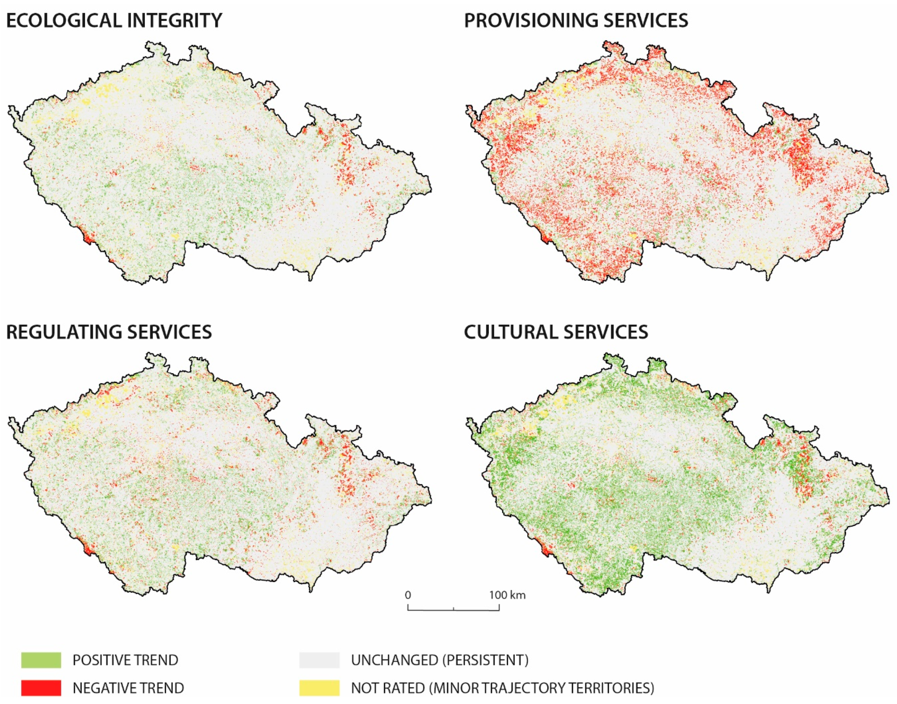
Figure 1 shows the spatial distribution of the classified trend development for selected ESs.
The largest area is the area of change in the category of non-irrigated arable land to pastures, with 3601 patches with a total area of 2269.18 ha. In terms of capacity for providing ecological integrity, both categories were rated as level 3, relevant capacity, so there was no change in capacity level over time. In terms of capacity level for provisioning services, after a category change, the level decreased from 2 (relevant capacity) to 1 (low relevant capacity) and remains at level 1 for regulating services. For cultural services it rises from level 1, low relevant capacity, to 2, relevant capacity. Examples of a downward trend in capacity levels for all analyzed ecosystem services were found for transitions from the non-irrigated arable land category to discontinuous urban fabric, or coniferous forest transitioning to transitional woodland-shrub. On the other hand, an upward trend in capacity levels for all monitored ecosystem services at all-time horizons was found in the transitional woodland-shrub category, and transitioning to coniferous forest or mixed forest.
The results also show that the territory of the Czech Republic has a higher capacity for the provision of ecological integrity than for the remaining three evaluated services, as the vast majority of the territory had higher levels of relevant capacity (3–5), but its area decreased in the observed period and the area with lower potential increased. When assessing the potential for providing provisioning services, it can be seen that the whole territory was at lower levels of relevant capacity (0–2), and development was leading to an increase in areas of low relevant capacity. The development of regulating service potential over time led to a rise in areas of higher relevant capacity at the expense of lower levels, even though the highest level does not occur. In terms of cultural service provisioning capacity, the territory includes all levels of potential, with a significant decrease in level 1 (low relevant capacity) during the reporting period in favor of other levels, in particular 2 (relevant capacity) and 5 (very high relevant capacity).
4. Discussion
This paper provides a spatial ES assessment using five land cover datasets and presents an evaluation of the positive/negative trends according to an expert-based evaluation of the ES capacity. The use and structure of a landscape is a matrix that is crucial for provision of an ES [52]. An important trend of land cover changes in the studied area is the increase in the areas of artificial surfaces, forest and semi-natural areas, and inland waters during the study period. This trend is in line with the well-known trend of changes in the Central European cultural landscape [53,54]. Thus, the land cover analysis of agricultural areas, whose area decreased by 852 km2, was the largest change, with wetlands showing the smallest change. The most extensive categories of the observed area besides the largest category of non-irrigated arable land are coniferous forest, land principally occupied by agriculture, mixed forest, discontinuous urban fabric, broad-leaved forest, and pastures, with a total area of over 2000 km2 and high persistence, which positively influences the value of persistence of the whole territory. The area of categories with a persistence value higher than the value of the territory is 33,767.3 km2. Conversely, low-persistence categories have small areas of only tens of km2. The total area of categories with persistence that is lower than the value of the territory is 28,915.32 km2. If the category of non-irrigated arable land belonging to this group and occupying almost half of the monitored area is not included, the category area is only 1580.16 km2.
When interpreting the results, several methodological aspects need to be kept in mind.
All conclusions are valid for the input data scale. CLC’s spatial resolution corresponds to a scale of 1:100,000 and is thus not able to account for detailed landscape changes of tens of meters to hundreds of square meters [55]. On the other hand, these data represent a long and widely-used data base that retains the basic methodological elements of acquisition and is thus a very suitable data source for multi-temporal analyses [48,56]. The described development is not based on continuous data, but on data capturing the development in steps; “snapshots” at certain dates. Therefore, it cannot be ruled out that in some cases there could be a significant but short-term change in the land cover, and hence the degree of fulfillment of the selected ES could have changed. This “shortcoming” is well known in the literature, but it is still considered a common method with regards to data availability [57]. It is recommended to base the assessment of development on the longest possible time series, with sufficient horizons included in the analysis. In our case, we used five data layers with the same methodology and regular spacing for a period of 28 years. The assessment of the development is therefore based on the main trajectories—those that can be observed over an area of more than 100 hectares in total. The selection of the limiting area was tested under conditions of 10, 50, 100, and 500 hectares. The value of 100 hectares proved to be the best, as the ratio of the number of identified main trajectories to the area concerned produced the best results.
Spatial identification of persistent areas over five time periods is an innovative element of our study. It is important to remember that landscape development is a long-term issue, and only a stable and developed ecosystem can perform well [58]. An example of high persistence is the category of non-irrigated arable land, whose 5968 patches with an area of 27,335.15 ha occurred in the Czech Republic in all five monitored periods. This also means that the level of capacity for providing ecological integrity is medium throughout the observed period, for provisioning services it is relevant capacity, and for regulating services and cultural services it is low relevant capacity. Over time, the variable area, although currently classified as a good category for ES performance (e.g., mixed forest), cannot fulfill its function to the maximum in the short term after the change (these will be the initialization stages) [44,59]. The clear recommendation is therefore to focus landscape protection on persistent areas with good ES capacity [60].
We used expert tables created in Germany to evaluate the capacity of ES fulfillment. We have left this table unchanged for our analysis because (i) the physical-geographical situation is very similar to the Czech Republic; both countries are located in Central Europe, adjacent to each other. In their continental areas, they have very similar natural conditions. Coastal and marine services, where there could be a significant difference, were not taken into account. The work of the authors [16,32] of this methodology has proven its applicability throughout the entirety of Europe several times. (ii) The data for land cover description (CLC) are the same for both countries, and the definitions of the individual land cover categories are the same. A disadvantage is the fact that the evaluation is based only on the CLC category and does not take into account the current state of the landscape segment in any way.
In retrospective analysis, however, this cannot be done otherwise. Usually, there is no way to evaluate the current state of the habitat and correct the capacity values. However, for up-to-date data, the situation is different. It is possible to supplement the basic data with field mapping at control locations, and subsequently correct the data. An example of such an assessment is the BVM method, with a variant of individual habitat assessment [24,61]. The current trend in the assessment of landscape status and features is the analysis of multispectral satellite data with a high temporal resolution. For Europe, this includes data from the Sentinel-1 and Sentinel-2 satellites [62].
In this study, four groups of ecosystem services (ecological integrity, provisioning, regulating, and cultural services) were evaluated, based on work [18] at five time horizons in the Czech Republic.
Ecological integrity means the natural equilibrium state of the human ecosystem is not affected by human activity [51,63]. Changes in landscape coverage are reflected in a change in the level of capacity provision for ecosystem services [64]. A significant decrease in the capacity level is apparent, for example, in the change of the coniferous forest category to transitional woodland-shrub when assessing the level of capacity for regulating services from medium relevant capacity to no relevant capacity, or for the same category change when assessing the level of capacity for cultural services from high relevant capacity to relevant capacity. Conversely, a significant increase in the capacity level is apparent in the change of the transitional woodland-shrub category to coniferous forest or mixed forest when assessing the capacity level for regulating services from no relevant capacity to high relevant capacity, or for a category change of non-irrigated arable land to coniferous forest when assessing the level of capacity for cultural services from low relevant capacity to very high relevant capacity.
The results can be compared with a study of ecosystem services in the Czech Republic that was conducted in 2014 [65]. Comparing our partial data from 2012, we can see the same distribution of areas with different degrees of ES provision.
A similar study is the work on the development of the ES price in the Czech Republic in the period of 1845–2010. The study, however, focuses on a different period, uses other data, and mainly deals with only one small study area. However, the main trend—the increase in urbanized areas, which reduces the ability to fulfill ESs—is also identifiable [66].
The results achieved at the national level illustrate areas where attention must be paid to the protection of the current state of the landscape, and where the protection of the territory needs to be increased in order to reduce negative trends. To accurately identify sites, the logical step would be to overlap the results with the existing network of protected areas. This was initially considered as the last step of this analysis but has been dropped. The CLC data is too rough to propose practical measures through a change to the nature conservation regime [67]. Such a study should be carried out at the level of habitats, whose mapping within the Natura2000 network fully corresponds to the scale of delimitation of protected areas in the Czech Republic and the legislative requirements of spatial planning [68]. This analysis has been carried out for the present [23], and a multi-temporal extension is under preparation. These results will serve as a significant contribution to understanding the situation of the 2016 Biodiversity Conservation Strategy [69] on a national level. Based on the results, it is possible to formulate several recommendations for several national strategies. Above all, it is necessary to limit further growth of urbanized areas, which reduces the capacity of all four services. It is also necessary to limit the conversion of forest cultures to agriculture, which significantly reduces the capacity of regulating services.
5. Conclusions
Environmental management is strongly influenced by the historical development of the territory and particularly by environmental policy. The territory of the Czech Republic underwent significant changes in the category of land use in the monitored period, which has affected the potential for ES provision. The results of this study show different development trends for the selected services.
When assessing the landscape’s ability to provide services according to selected development trajectories, it follows that the territory of the Czech Republic had the highest capacity to provide ecological integrity in 1990–2006, and then this capacity declined slightly. The level of provisioning services gradually decreased over the period under review, and the level of regulatory services and cultural services steadily increased until 2006, before declining again. From a spatial point of view, the worst development trend is for provisioning services, where negative development is represented almost all over the country. On the contrary, cultural services show the most areas with a positive trend, mainly in the western part of the territory. Ecological integrity and regulating services have similar spatial characteristics of development. The results achieved by long-term data analysis could lead to a more efficient concept of environmental management, by identifying areas where attention must be paid to the protection of the current state of the landscape, and where the protection of the territory needs to be increased in order to reduce negative trends. Based on the results, it is possible to formulate several recommendations for several national strategies. Above all, it is necessary to limit further growth of urbanized areas, which reduces the capacity of all four services. It is also necessary to limit the conversion of forest cultures to agriculture, which significantly reduces the capacity for regulating services.
Author Contributions
Conceptualization, V.P., I.M. and H.K.; Methodology, V.P.; Software, V.P., I.M. and E.T.; GIS Analysis, V.P, H.K. and E.T.; Resources, A.V. and I.M.; Writing—original draft preparation, V.P and H.K; Writing—review and editing, E.T.; visualization, A.V.
Funding
This research received no external funding.
Conflicts of Interest
The authors declare no conflict of interest.
References
- Millennium Ecosystem Assessment. Ecosystems and Human Well-Being; Island Press: Washington, DC, USA, 2005. [Google Scholar]
- Müller, F.; Burkhard, B. An ecosystem based framework to link landscape structures, functions and services. In Multifunctional Land Use: Meeting Future Demands for Landscape Goods and Services; Mander, Ü., Wiggering, H., Helming, K., Eds.; Springer: Berlin/Heidelberg, Germany, 2007; pp. 37–63. [Google Scholar]
- Vaz, A.S.; Kueffer, C.; Kull, C.A.; Richardson, D.M.; Vicente, J.R.; Kühn, I.; Schröter, M.; Hauck, J.; Bonn, A.; Honrado, J.P. Integrating ecosystem services and disservices: Insights from plant invasions. Ecosyst. Serv. 2017, 23, 94–107. [Google Scholar] [CrossRef]
- De Groot, R.S.; Wilson, M.A.; Boumans, R. A typology for the classification, description and valuation of ecosystem functions, goods and services. Ecol. Econ. 2002, 41, 393–408. [Google Scholar] [CrossRef] [Green Version]
- Costanza, R. Ecosystem services: Multiple classification systems are needed. Biol. Conserv. 2008, 141, 350–352. [Google Scholar] [CrossRef]
- TEEB. The Economics of Ecosystem and Biodiversity for Local and Regional Policy Makers. Report 207. 2010. Available online: http://www.teebweb.org/wp-content/uploads/Study> and Reports/Reports/Local and Regional Policy Makers/D2 Report/TEEB_Local_Policy-Makers_Report.pdf (accessed on 18 June 2019).
- Haines-Young, R.; Potschin, M. The links between biodiversity, ecosystem services and human well-being. In Ecosystem Ecology: A New Synthesis; Raffaeli, D., Frid, C., Eds.; Cambridge University Press: Cambridge, UK, 2010; pp. 110–139. [Google Scholar]
- De Groot, R.S.; Alkemade, R.; Braat, L.; Hein, L.; Willemen, L. Challenges in integrating the concept of ecosystem services and values in landscape planning, management and decision making. Ecol. Complex. 2010, 7, 260–272. [Google Scholar] [CrossRef]
- Machar, I. Protection of nature and landscapes in the Czech Republic Selected current issues and possibilities of their solution. In Ochrana Prirody a Krajiny v Ceske Republikce; Palacký University Olomouc: Olomouc, Czechia, 2012; Accession Number: WOS:000334387900001. [Google Scholar]
- Opršal, Z.; Harmáček, J.; Pavlík, P.; Machar, I. What factors can influence the expansion of protected areas around the world in the context of international environmental and development goals. Probl. Ekorozwoju 2018, 13, 145–157. [Google Scholar]
- Heal, G. Valuing ecosystem services. Ecosystems 2000, 3, 24–30. [Google Scholar] [CrossRef]
- De Groot, R.S. Function-analysis and valuation as a tool to assess land use conflicts in planning for sustainable, multi-functional landscapes. Landsc. Urban. Plann. 2016, 75, 175–186. [Google Scholar] [CrossRef]
- Castro, A.J.; Martín-López, B.; López, E.; Plieninger, T.; Alcaraz-Segura, D.; Vaughn, C.C.; Cabello, J. Do protected areas networks ensure the supply of ecosystem services? Spatial patterns of two nature reserve systems in semi-arid Spain. Appl. Geogr. 2015, 60, 1–9. [Google Scholar] [CrossRef]
- Cimon-Morin, J.; Darveau, M.; Poulin, M. Fostering synergies between ecosystem services and biodiversity in conservation planning: A review. Biol. Conserv. 2013, 166, 144–154. [Google Scholar] [CrossRef]
- Vihervaara, P.; Rönkä, M.; Walls, M. Trends in ecosystem service research: Early steps and current drivers. Ambio 2010, 39, 314–324. [Google Scholar] [CrossRef]
- Burkhard, B.; Kandziora, M.; Hou, Y.; Müller, F. Ecosystem Service Potentials, Flows and Demands–Concepts for Spatial Localisation, Indication and Quantification. Landsc. Online 2014, 34, 1–32. [Google Scholar] [CrossRef]
- Lee, H.; Lautenbach, S. A quantitative review of relationships between ecosystem services. Ecol. Indic. 2016, 66, 340–351. [Google Scholar] [CrossRef]
- Burkhard, B.; Kroll, F.; Müller, F.; Windhorst, W. Landscapes’ Capacities to Provide Ecosystem Services—A Concept for Land-Cover Based Assessments. Landsc. Online 2009, 15, 1–22. [Google Scholar] [CrossRef]
- Wangai, P.W.; Burkhard, B.; Muuller, F. Quantifying and mapping land use changes and regulating ecosystem service potentials in a data-scarce peri-urban region in Kenya. Int. J. Biodivers. Sci.Ecosyst. Serv. Manag. 2019. [Google Scholar] [CrossRef]
- Kareiva, P.; Marvier, M. What is conservation science? Articles 2012, 62, 962–969. [Google Scholar] [CrossRef]
- Bennett, E.M.; Peterson, G.D.; Gordon, L.J. Understanding relationships among multiple ecosystem services. Ecol. Lett. 2009, 12, 1–11. [Google Scholar] [CrossRef] [PubMed]
- Kati, V.; Hovardas, T.; Dieterich, M.; Ibisch, P.L.; Mihok, B.; Selva, N. The challenge of implementing the European network of protected areas Natura 2000. Conserv. Biol. 2015, 29, 260–270. [Google Scholar] [CrossRef]
- Pechanec, V.; Machar, I.; Pohanka, T.; Opršal, Z.; Petrovič, F.; Švajda, J.; Šálek, L.; Chobot, K.; Filippovová, J.; Cudlín, P.; et al. Effectiveness of Natura 2000 system for habitat types protection: A case study from the Czech Republic. Nat. Conserv. 2017, 24, 21–41. [Google Scholar] [CrossRef]
- Cudlín, P.; Pechanec, V.; Štěrbová, L.; Cudlín, O.; Purkyt, J. Integrated approach to the mitigation of biodiversity lost in Central Europe. In Ecological Integrity and Land Use: Sovereignty, Governance, Displacements and Land Grabs; Westra, L., Bosselmann, K., Zabrano, V., Eds.; Nova Science Publishers: New York, NY, USA, 2009; pp. 75–86. [Google Scholar]
- Kienast, F.; Bolliger, J.; Potschin, M.; De Groot, R.S.; Verburg, P.H.; Heller, I.; Wascher, D.; HainesYoung, R. Assessing landscape functions with broad-scale environmental data: Insights gained from a prototype development for europe. Environ. Manag. 2009, 44, 1099–1120. [Google Scholar] [CrossRef]
- Chan, K.M.A.; Shaw, M.R.; Cameron, D.R.; Underwood, E.C.; Daily, G.C. Conservation planning for ecosystem services. PLoS Biol. 2006, 4, 2139–2152. [Google Scholar] [CrossRef]
- Jaeger, J.A.G. Landscape division, splitting index, and effective mesh size: New measures of landscape fragmentation. Landsc. Ecol. 2000, 15, 115–130. [Google Scholar] [CrossRef]
- Maes, J.; Egoh, B.; Willemen, L.; Liquete, C.; Vihervaara, P.; Schagner, J.P.; Grizzetti, B. Mapping ecosystem services for policy support and decision making in the European Union. Ecosyst. Serv. 2012, 1, 31–39. [Google Scholar] [CrossRef]
- Schulp, C.J.E.; Burkhard, B.; Maes, J.; Van Vliet, J.; Verburg, P.H. Uncertainties in ecosystem service maps: A comparison on the European scale. PLoS ONE 2014, 9, e109643. [Google Scholar] [CrossRef] [PubMed]
- Kopperoinen, L.; Itkonen, P.; Niemela, J. Using expert knowledge in combining green infrastructure and ecosystem services in land use planning: An insight into a new place-based methodology. Landsc. Ecol. 2014, 29, 1361–1375. [Google Scholar] [CrossRef]
- Vrebos, D.; Staes, J.; Vandenbroucke, T.; D’Haeyer, T.; Johnston, R.; Muhumuza, M.; Meire, P. Mapping ecosystem service flows with land cover scoring maps for data-scarce regions. Ecosyst. Serv. 2015, 13, 28–40. [Google Scholar] [CrossRef]
- Jacobs, S.; Burkhard, B.; Van Deale, T.; Staes, J.; Schneiders, A. The matrix reloaded: A review of expert knowledge for mapping ecosystem Services. Ecol. Model. 2015, 295, 21–30. [Google Scholar] [CrossRef]
- Müller, F.; de Groot, R.; Willemen, L. Ecosystem Services at the Landscape Scale: The Need for Integrative Approaches. Landsc. Online 2010, 23, 1–11. [Google Scholar] [CrossRef]
- Crossman, N.D.; Burkhard, B.; Nedkov, S.; Willemen, L.; Petz, K.; Palomo, I.; Drakou, E.G.; MartínLopez, B.; McPhearson, T.; Boyanova, K.; et al. A blueprint for mapping and modelling ecosystem services. Ecosyst. Serv. 2013, 4, 4–14. [Google Scholar] [CrossRef]
- Eigenbrod, F.; Armsworth, P.R.; Anderson, B.J.; Heinemeyer, A.; Gillings, S.; Roy, D.B.; Thomas, C.D.; Gaston, K.J. The impact of proxy-based methods on mapping the distribution of ecosystem services. J. Appl. Ecol. 2010, 47, 377–385. [Google Scholar] [CrossRef]
- Costanza, R.; D’Arge, R.; De Groot, R.; Farber, S.; Grasso, M.; Hannon, B.; van den Belt, M. The value of the world’s ecosystem services and natural capital. Nature 1997, 387, 253–260. [Google Scholar] [CrossRef]
- Troy, A.; Wilson, M.A. Mapping ecosystem services: Practical challenges and opportunities in linking GIS and value transfer. Ecol. Econ. 2006, 60, 435–449. [Google Scholar] [CrossRef]
- Lavorel, S.; Grigulis, K. How fundamental plant functional trait relationships scale-up to trade-offs and synergies in ecosystem services. J. Ecol. 2012, 100, 128–140. [Google Scholar] [CrossRef]
- Tallis, H.; Polasky, S. Mapping and valuing ecosystem services as an approach for conservation and natural-resource management. Ann. N. Y. Acad. Sci. 2009, 1162, 265–283. [Google Scholar] [CrossRef] [PubMed]
- Villa, F.; Ceroni, M.; Bagstad, K.; Johnson, G.; Krivov, S. ARIES (ARtificial Intelligence for Ecosystem Services): A new tool for ecosystem services assessment, planning, and valuation. In Proceedings of the 11th Annual BIOECON Conference on Economic Instruments to Enhance the Conservation and Sustainable Use of Biodiversity, Venice, Italy, 21–22 September 2009; pp. 1–10. [Google Scholar]
- Fisher, B.; Turner, R.K.; Morling, P. Defining and classifying ecosystem services for decision making. Ecol. Econ. 2009, 68, 643–653. [Google Scholar] [CrossRef] [Green Version]
- Vondráková, A.; Vávra, A.; Voženílek, V. Climatic regions of the Czech Republic. J. Maps 2013, 9, 425–430. [Google Scholar] [CrossRef] [Green Version]
- Kilianová, H.; Pechanec, V.; Brus, J.; Kirchner, K.; Machar, I. Analysis of the development of land use in the Morava River floodplain, with special emphasis on the landscape matrix. Morav. Geogr. Rep. 2017, 25, 46–59. [Google Scholar] [CrossRef] [Green Version]
- Simon, J.; Machar, I.; Brus, J.; Pechanec, V. Combining a growth-simulation model with acoustic-wood tomography as a decision-support tool for adaptive management and conservation of forest ecosystems. Ecol. Inform. 2015, 30, 309–312. [Google Scholar] [CrossRef]
- Samec, P.; Vozenilek, V.; Vondrakova, A.; Macku, J. Diversity of forest soils and bedrock in soil regions of the Central-European highlands (Czech Republic). Catena 2018, 160, 95–102. [Google Scholar] [CrossRef]
- Machar, I.; Vozenilek, V.; Kirchner, K.; Vlckova, V.; Bucek, A. Biogeographic model of climate conditions for vegetation zones in Czechia. Geografie 2017, 122, 64–82. [Google Scholar] [Green Version]
- Tuček, P.; Caha, J.; Janoška, Z.; Vondráková, A.; Samec, P.; Bojko, J.; Voženílek, V. Forest vulnerability zones in the Czech Republic. J. Maps 2014, 10, 179–182. [Google Scholar] [CrossRef]
- Pechanec, V.; Mráz, A.; Benc, A.; Cudlín, P. Analysis of spatiotemporal variability of C-factor derived from remote sensing data. J. Appl. Remote Sens. 2018, 12, 016022. [Google Scholar] [CrossRef]
- Pechanec, V.; Purkyt, J.; Benc, A.; Nwaogu, C.; Štěrbová, L.; Cudlín, P. Modelling of the carbon sequestration and its prediction under climate change. Ecol. Inform. 2018, 47, 50–54. [Google Scholar] [CrossRef]
- Pechanec, V.; Vávra, A.; Hovorková, M.; Brus, J.; Kilianová, H. Analyses of moisture parameters and biomass of vegetation cover in southeast Moravia. Int. J. Remote Sens. 2014, 35, 967–987. [Google Scholar] [CrossRef]
- Angermeier, P.L.; Karr, J.R. Biological integrity versus biological diversity as policy directives: Protecting biotic resources. BioScience 1994, 44, 690–697. [Google Scholar] [CrossRef]
- Zeller, K.A.; McGarigal, K.; Whiteley, A.R. Estimating landscape resistance to movement: A review. Landsc. Ecol. 2012, 27, 777–797. [Google Scholar] [CrossRef]
- Kilianova, H.; Pechanec, V.; Svobodova, J.; Machar, I. Analysis of the evolution of the floodplain forests in the aluvium of the Morava river. In Proceedings of the 12th International Multidisciplinary Scientific Geoconference, SGEM 2012, Albena, Bulgaria, 17–23 June 2012; Volume IV, pp. 1–8, Accession Number: WOS:000348535300001. [Google Scholar]
- Machar, I. Changes in ecological stability and biodiversity in a floodplain landscape. In Applying Landscape Ecology in Conservation and Management of the Floodplain Forest (Czech. Republic); Palacky University: Olomouc, Czech Republic, 2012; pp. 73–87. [Google Scholar]
- Brus, J.; Pechanec, V.; Machar, I. Depiction of uncertainty in the visually interpreted land cover data. Ecol. Inform. 2018, 47, 10–13. [Google Scholar] [CrossRef]
- Martínez-Fernández, J.; Ruiz-Benito, P.; Bonet, A.; Gómez, C. Methodological variations in the production of CORINE land cover and consequences for long-term land cover change studies. The case of Spain. Int. J. Remote Sens. 2019. [Google Scholar] [CrossRef]
- Mugiraneza, T.; Ban, Y.; Haas, J. Urban land cover dynamics and their impact on ecosystem services in Kigali, Rwanda using multi-temporal Landsat data. Remote Sens. Appl. Soc. Environ. 2019, 13, 234–246. [Google Scholar] [CrossRef]
- Bommarco, R.; Kleijn, D.; Potts, S.G. Ecological intensification: Harnessing ecosystem services for food security. Trends Ecol. Evol. 2013, 28, 230–238. [Google Scholar] [CrossRef]
- Maděra, P.; Packova, P. Primary succession of white willow communities in the supraregional biocorridor in the middle water reservoir of Nove Mlyny. Ekol. Bratisl. 2004, 23, 191–204. [Google Scholar]
- Pejchar, L.; Morgan, P.M.; Caldwell, M.R.; Palmer, C.; Daily, G.C. Evaluating the potential for conservation development: Biophysical, economic, and institutional perspectives. Conserv. Biol. 2007, 21, 69–78. [Google Scholar] [CrossRef]
- Seják, J.; Dejmal, I.; Petříček, V.; Cudlín, P.; Míchal, I.; Černý, K.; Kučera, T.; Vyskot, I.; Strejček, J.; Cudlínová, E.; et al. Valuation and Prizing of Biotopes of the Czech. Republic; Czech Ecological Institute: Prague, Czech Republic, 2003; p. 422. (In Czech) [Google Scholar]
- Haas, J.; Ban, Y. Sentinel-1A SAR and sentinel-2A MSI data fusion for urban ecosystem service mapping. Remote Sens. Appl. Soc. Environ. 2017, 8, 41–53. [Google Scholar] [CrossRef]
- Kopecka, V.; Machar, I.; Bucek, A.; Kopecky, A. The Impact of Climate Changes on Sugar Beet Growing Conditions in the Czech Republic. Listy Cukrov. Repar. 2013, 129, 326–329. [Google Scholar]
- Yang, L.; Zhang, L.; Li, Y.; Wu, S. Landscape and urban planning water-related ecosystem services provided by urban green space: A case study in Yixing City (China). Landsc. Urban. Plan. 2015, 136, 40–51. [Google Scholar] [CrossRef]
- Frélichová, J.; Vačkář, D.; Pártl, A.; Loučková, B.; Harmáčková, Z.V.; Lorencová, E. Integrated assessment of ecosystem services in the Czech Republic. Ecosyst. Serv. 2014, 8, 110–117. [Google Scholar] [CrossRef]
- Frélichová, J.; Fanta, J. Ecosystem service availability in view of long-term land-use changes: A regional case study in the Czech Republic. Ecosyst. Health Sustain. 2015, 1, 1–15. [Google Scholar] [CrossRef]
- Bach, M.; Breuer, L.; Frede, H.G.; Huisman, J.A.; Otte, A.; Waldhardt, R. Accuracy and congruency of three different digital land-use maps. Landsc. Urban Plan. 2006, 78, 289–299. [Google Scholar] [CrossRef]
- Burian, J.; Šťastný, S.; Brus, J.; Pechanec, V.; Voženílek, V. Urban Planner: Model for optimal land use scenario modelling. Geografie 2015, 120, 330–353. [Google Scholar]
- National Biodiversity Strategy of the Czech Republic—2016–2025, 2nd ed.; Ministry of the Environment: Prague, Czech Republic, 2016. Available online: https://www.cbd.int/doc/world/cz/cz-nbsap-v2-en.pdf (accessed on 17 July 2019).
Figure 1.
Spatial distribution of the trend development for selected ESs.


Table 1.
The development of land cover in the Czech Republic over five periods from 1990 to 2018.
| TAG | Land Cover Category | 1990 | 2000 | 2006 | 2012 | 2018 1 |
|---|---|---|---|---|---|---|
| 111 | Continuous urban fabric | 14.64 | 14.64 | 15.67 | 15.67 | 15.7 |
| 112 | Discontinuous urban fabric | 3578.5 | 3625.85 | 3783.53 | 3825.26 | 3947.14 |
| 121 | Industrial or commercial units | 521.2 | 547.73 | 602.11 | 631.01 | 656.45 |
| 122 | Road and rail networks and associated land | 48.07 | 52.73 | 62.6 | 72.09 | 71.88 |
| 123 | Port areas | 1.5 | 1.5 | 0.79 | 0.79 | 0.79 |
| 124 | Airports | 56.09 | 56.27 | 53.31 | 53.01 | 54.69 |
| 131 | Mineral extraction sites | 180.63 | 171.02 | 165.56 | 169.35 | 179.59 |
| 132 | Dump sites | 154.61 | 138.86 | 94.55 | 79.4 | 59.94 |
| 133 | Construction sites | 21.24 | 8.57 | 23.44 | 10.9 | 15.12 |
| 141 | Green urban areas | 65.26 | 65.55 | 66.88 | 66.58 | 67.15 |
| 142 | Sport and leisure facilities | 117.71 | 127.33 | 158 | 173.34 | 185.86 |
| 211 | Non-irrigated arable land | 35541.03 | 32621.67 | 29891.77 | 28991.31 | 28705.47 |
| 221 | Vineyards | 110.77 | 119.42 | 156.92 | 164.66 | 169.04 |
| 222 | Fruit trees and berry plantations | 328.21 | 326.44 | 313.9 | 294.06 | 262.8 |
| 231 | Pastures | 2527.62 | 5317.05 | 7185.62 | 7943.93 | 8067.84 |
| 242 | Complex cultivation patterns | 415.34 | 429.53 | 476.2 | 472.53 | 473.94 |
| 243 | Land principally occupied by agriculture, with significant areas of natural vegetation | 6736.18 | 6747.69 | 7079.4 | 7114.46 | 7128.05 |
| 311 | Broad-leaved forest | 2495.24 | 2527.4 | 2783.22 | 2838.85 | 2833.73 |
| 312 | Coniferous forest | 16552.1 | 16992.92 | 17226.97 | 17126.26 | 16658.11 |
| 313 | Mixed forest | 5854.94 | 6042.24 | 6173.85 | 6336.97 | 6436.94 |
| 321 | Natural grasslands | 404.64 | 392.04 | 261.97 | 256.63 | 251.92 |
| 322 | Moors and heathland | 26.52 | 27.39 | 18.15 | 18.15 | 22.58 |
| 324 | Transitional woodland-shrub | 2486.74 | 1869.7 | 1598.99 | 1528.7 | 1909.01 |
| 332 | Bare rocks | 2.1 | 2.1 | 1.48 | 1.48 | 1.97 |
| 333 | Sparsely vegetated areas | 0 | 0 | 1.15 | 1.45 | 3.79 |
| 334 | Burnt areas | 1.17 | 0 | 0 | 0 | 0 |
| 411 | Inland marshes | 53.54 | 53.36 | 60.84 | 60.84 | 60.99 |
| 412 | Peat bogs | 37.5 | 37.11 | 46.72 | 45.52 | 45.68 |
| 511 | Water courses | 42.8 | 43.01 | 44.78 | 45.16 | 46.56 |
| 512 | Water bodies | 492.89 | 509.67 | 520.43 | 530.44 | 536.08 |
| Total | 78868.8 | 78868.8 | 78868.8 | 78868.8 | 78868.8 |
1 The area of each year is in km2.
Table 2.
The persistence of individual land cover classes.
| Land Cover Category | Area (km2) | Percentage of Persistence (%) |
|---|---|---|
| 111 Continuous urban fabric | 13.01 | 88.88 |
| 112 Discontinuous urban fabric | 3337.49 | 93.27 |
| 121 Industrial or commercial units | 481.06 | 92.3 |
| 122 Road and rail networks and associated land | 45.07 | 93.75 |
| 123 Port areas | 0.76 | 50.87 |
| 124 Airports | 49.22 | 87.75 |
| 131 Mineral extraction sites | 86.05 | 47.64 |
| 132 Dump sites | 40.6 | 26.26 |
| 141 Green urban areas | 57.09 | 87.49 |
| 142 Sport and leisure facilities | 88.55 | 75.22 |
| 211 Non-irrigated arable land | 27335.16 | 76.91 |
| 221 Vineyards | 77.76 | 70.2 |
| 222 Fruit trees and berry plantations | 159.79 | 48.69 |
| 231 Pastures | 2086.58 | 82.55 |
| 242 Complex cultivation patterns | 316.21 | 76.13 |
| 243 Land principally occupied by agriculture …. | 5440.98 | 80.77 |
| 311 Broad-leaved forest | 2320.08 | 92.98 |
| 312 Coniferous forest | 14368.4 | 86.81 |
| 313 Mixed forest | 5034.2 | 85.98 |
| 321 Natural grasslands | 209.84 | 51.86 |
| 322 Moors and heathland | 12.3 | 46.36 |
| 324 Transitional woodland-shrub | 549.21 | 22.09 |
| 332 Bare rocks | 0.52 | 24.74 |
| 411 Inland marshes | 38.57 | 72.04 |
| 412 Peat bogs | 31.68 | 84.49 |
| 511 Water courses | 39.46 | 92.18 |
| 512 Water bodies | 462.98 | 93.93 |
| Total | 62682.62 | 79.48 |
Table 3.
Development of the area (km2) of classes of ES capacity for ecological integrity.
| Capacity | 1990 | 2000 | 2006 | 2012 | 2018 | Persistent |
|---|---|---|---|---|---|---|
| No relevant capacity | 558.58 | 572.44 | 642.01 | 658.37 | 688.06 | 494.83 |
| Low relevant capacity | 4021.17 | 4046.83 | 4162.18 | 4202.04 | 4319 | 3558.95 |
| Relevant capacity | 228.48 | 246.75 | 314.92 | 338 | 354.9 | 166.31 |
| Medium relevant capacity | 48636.07 | 47930.31 | 47177.97 | 46987.17 | 47196.9 | 36447.46 |
| High relevant capacity | 19569.54 | 20030.22 | 20397.87 | 20346.25 | 19873.01 | 16980.87 |
| Very high relevant capacity | 5854.94 | 6042.24 | 6173.85 | 6336.97 | 6436.94 | 5034.2 |
Table 4.
Development of the area (km2) of classes of ES capacity for provisioning services.
| Capacity | 1990 | 2000 | 2006 | 2012 | 2018 | Persistent |
|---|---|---|---|---|---|---|
| No relevant capacity | 7802.37 | 7230.42 | 7093.67 | 7095.84 | 7635.72 | 5067.91 |
| Low relevant capacity | 3886.92 | 6706.45 | 8619.92 | 9365.11 | 9470.79 | 3115.89 |
| Relevant capacity | 67179.49 | 64931.92 | 63155.21 | 62407.85 | 61762.3 | 54498.82 |
Table 5.
Development of the area (km2) of classes of ES capacity for regulating services.
| Capacity | 1990 | 2000 | 2006 | 2012 | 2018 | Persistent |
|---|---|---|---|---|---|---|
| No relevant capacity | 7177.26 | 6608.39 | 6560.1 | 6553.77 | 7085.11 | 4680.75 |
| Low relevant capacity | 45938.83 | 45861.5 | 45423.08 | 45337.75 | 45210.95 | 35827.01 |
| Relevant capacity | 812.91 | 799.23 | 654.86 | 629.68 | 598.29 | 420.5 |
| Medium relevant capacity | 37.5 | 37.11 | 46.72 | 45.52 | 45.68 | 31.68 |
| High relevant capacity | 24902.28 | 25562.56 | 26184.04 | 26302.08 | 25928.78 | 21722.68 |
Table 6.
Development of the area (km2) of classes of ES capacity for cultural services.
| Capacity | 1990 | 2000 | 2006 | 2012 | 2018 | Persistent |
|---|---|---|---|---|---|---|
| No relevant capacity | 4629.69 | 4669.03 | 4862.76 | 4918.98 | 5065.29 | 4091.07 |
| Low relevant capacity | 35957.87 | 33052.7 | 30368.76 | 29464.63 | 29180.2 | 27652.13 |
| Relevant capacity | 5081.72 | 7254.4 | 8852.97 | 9540.69 | 10045.97 | 2693.4 |
| Medium relevant capacity | 7697.51 | 7712.92 | 7970.19 | 8003.15 | 7997.67 | 5976.92 |
| High relevant capacity | 37.5 | 37.11 | 46.72 | 45.52 | 45.68 | 31.68 |
| Very high relevant capacity | 25464.49 | 26142.63 | 26767.4 | 26895.83 | 26534 | 22237.42 |
Table 7.
Main trajectories of land cover development in the Czech Republic.
| No. | Development Trajectory (1990-2000-2006-2012-2018) | Number of Patches this Trajectory | Area of Patches this Trajectory (ha) |
|---|---|---|---|
| 1 | 211-211-112-112-112 | 18894 | 174.79 |
| 2 | 211-211-211-211-112 | 6315 | 111.09 |
| 3 | 211-211-211-211-231 | 6450 | 253.91 |
| 4 | 211-211-211-231-231 | 1511 | 707.68 |
| 5 | 211-211-231-231-231 | 9566 | 1856.04 |
| 6 | 211-211-243-243-243 | 29578 | 878.037 |
| 7 | 211-211-312-312-312 | 31691 | 158.79 |
| 8 | 211-231-211-211-211 | 2360 | 209.79 |
| 9 | 211-231-231-231-231 | 3601 | 2269.18 |
| 10 | 243-243-211-211-211 | 24065 | 226.13 |
| 11 | 243-243-231-231-231 | 11624 | 350.50 |
| 12 | 243-243-312-312-312 | 14355 | 108.42 |
| 13 | 312-312-312-312-324 | 2222 | 473.53 |
| 14 | 312-312-312-324-324 | 254 | 172.40 |
| 15 | 312-312-313-313-313 | 10962 | 374.95 |
| 16 | 312-324-312-312-312 | 3218 | 124.82 |
| 17 | 312-324-324-324-324 | 729 | 171.94 |
| 18 | 313-313-311-311-311 | 4266 | 230.60 |
| 19 | 313-313-312-312-312 | 9649 | 265.86 |
| 20 | 324-312-312-312-312 | 3212 | 807.92 |
| 21 | 324-313-313-313-313 | 683 | 189.24 |
| 22 | 324-324-312-312-312 | 5132 | 227.73 |
Table 8.
Trend of development capacity for ecological integrity and provisioning services for 22 main trajectories.
Table 8.
Trend of development capacity for ecological integrity and provisioning services for 22 main trajectories.
| No. | Ecological Integrity | Provisioning Services | ||||||||||
|---|---|---|---|---|---|---|---|---|---|---|---|---|
| 1990 | 2000 | 2006 | 2012 | 2018 | Trend | 1990 | 2000 | 2006 | 2012 | 2018 | Trend | |
| 1 | 3 | 3 | 1 | 1 | 1 | negative | 2 | 2 | 0 | 0 | 0 | negative |
| 2 | 3 | 3 | 3 | 3 | 1 | negative | 2 | 2 | 2 | 2 | 0 | negative |
| 3 | 3 | 3 | 3 | 3 | 3 | unchanged | 2 | 2 | 2 | 2 | 1 | negative |
| 4 | 3 | 3 | 3 | 3 | 3 | unchanged | 2 | 2 | 2 | 1 | 1 | negative |
| 5 | 3 | 3 | 3 | 3 | 3 | unchanged | 2 | 2 | 1 | 1 | 1 | negative |
| 6 | 3 | 3 | 3 | 3 | 3 | unchanged | 2 | 2 | 2 | 2 | 2 | unchanged |
| 7 | 3 | 3 | 4 | 4 | 4 | positive | 2 | 2 | 2 | 2 | 2 | unchanged |
| 8 | 3 | 3 | 3 | 3 | 3 | unchanged | 2 | 1 | 2 | 2 | 2 | negative |
| 9 | 3 | 3 | 3 | 3 | 3 | unchanged | 2 | 1 | 1 | 1 | 1 | negative |
| 10 | 3 | 3 | 2 | 2 | 2 | negative | 2 | 2 | 0 | 0 | 0 | negative |
| 11 | 3 | 3 | 3 | 3 | 3 | unchanged | 2 | 2 | 1 | 1 | 1 | negative |
| 12 | 3 | 3 | 4 | 4 | 4 | positive | 2 | 2 | 2 | 2 | 2 | unchanged |
| 13 | 4 | 4 | 4 | 4 | 3 | negative | 2 | 2 | 2 | 2 | 0 | negative |
| 14 | 4 | 4 | 4 | 3 | 3 | negative | 2 | 2 | 2 | 0 | 0 | negative |
| 15 | 4 | 4 | 5 | 5 | 5 | positive | 2 | 2 | 2 | 2 | 2 | unchanged |
| 16 | 4 | 3 | 4 | 4 | 4 | negative | 2 | 0 | 2 | 2 | 2 | negative |
| 17 | 4 | 3 | 3 | 3 | 3 | negative | 2 | 0 | 0 | 0 | 0 | negative |
| 18 | 5 | 5 | 4 | 4 | 4 | negative | 2 | 2 | 2 | 2 | 2 | unchanged |
| 19 | 5 | 5 | 4 | 4 | 4 | negative | 2 | 2 | 2 | 2 | 2 | unchanged |
| 20 | 3 | 4 | 4 | 4 | 4 | positive | 0 | 2 | 2 | 2 | 2 | positive |
| 21 | 3 | 4 | 4 | 4 | 4 | positive | 0 | 2 | 2 | 2 | 2 | positive |
| 22 | 3 | 3 | 4 | 4 | 4 | positive | 0 | 0 | 2 | 2 | 2 | positive |
The value in the row represents the point scale of capacities to provide selected ecosystem services.
Table 9.
Trend of development capacity for regulating services and cultural services for 22 main trajectories.
Table 9.
Trend of development capacity for regulating services and cultural services for 22 main trajectories.
| No. | Regulating Services | Cultural Services | ||||||||||
|---|---|---|---|---|---|---|---|---|---|---|---|---|
| 1990 | 2000 | 2006 | 2012 | 2018 | Trend | 1990 | 2000 | 2006 | 2012 | 2018 | Trend | |
| 1 | 1 | 1 | 0 | 0 | 0 | negative | 1 | 1 | 0 | 0 | 0 | negative |
| 2 | 1 | 1 | 1 | 1 | 0 | negative | 1 | 1 | 1 | 1 | 0 | negative |
| 3 | 1 | 1 | 1 | 1 | 1 | unchanged | 1 | 1 | 1 | 1 | 2 | positive |
| 4 | 1 | 1 | 1 | 1 | 1 | unchanged | 1 | 1 | 1 | 2 | 2 | positive |
| 5 | 1 | 1 | 1 | 1 | 1 | unchanged | 1 | 1 | 2 | 2 | 2 | positive |
| 6 | 1 | 1 | 1 | 1 | 1 | unchanged | 1 | 1 | 3 | 3 | 3 | positive |
| 7 | 1 | 1 | 4 | 4 | 4 | positive | 1 | 1 | 5 | 5 | 5 | positive |
| 8 | 1 | 1 | 1 | 1 | 1 | unchanged | 1 | 2 | 1 | 1 | 1 | positive |
| 9 | 1 | 1 | 1 | 1 | 1 | unchanged | 1 | 2 | 2 | 2 | 2 | positive |
| 10 | 1 | 1 | 1 | 1 | 1 | unchanged | 3 | 3 | 3 | 3 | 3 | unchanged |
| 11 | 1 | 1 | 1 | 1 | 1 | unchanged | 3 | 3 | 2 | 2 | 2 | negative |
| 12 | 1 | 1 | 4 | 4 | 4 | positive | 3 | 3 | 5 | 5 | 5 | positive |
| 13 | 4 | 4 | 4 | 4 | 0 | negative | 5 | 5 | 5 | 5 | 2 | negative |
| 14 | 4 | 4 | 4 | 0 | 0 | negative | 5 | 5 | 5 | 2 | 2 | negative |
| 15 | 4 | 4 | 4 | 4 | 4 | unchanged | 5 | 5 | 5 | 5 | 5 | unchanged |
| 16 | 4 | 0 | 4 | 4 | 4 | negative | 5 | 2 | 5 | 5 | 5 | negative |
| 17 | 4 | 0 | 0 | 0 | 0 | negative | 5 | 2 | 2 | 2 | 2 | negative |
| 18 | 4 | 4 | 4 | 4 | 4 | unchanged | 5 | 5 | 5 | 5 | 5 | unchanged |
| 19 | 4 | 4 | 4 | 4 | 4 | unchanged | 5 | 5 | 5 | 5 | 5 | unchanged |
| 20 | 0 | 4 | 4 | 4 | 4 | positive | 2 | 5 | 5 | 5 | 5 | positive |
| 21 | 0 | 4 | 4 | 4 | 4 | positive | 2 | 5 | 5 | 5 | 5 | positive |
| 22 | 0 | 0 | 4 | 4 | 4 | positive | 2 | 2 | 5 | 5 | 5 | positive |
The value in the row represents the point scale of capacities to provide selected ecosystem services.
© 2019 by the authors. Licensee MDPI, Basel, Switzerland. This article is an open access article distributed under the terms and conditions of the Creative Commons Attribution (CC BY) license (http://creativecommons.org/licenses/by/4.0/).
Share and Cite
MDPI and ACS Style
Pechanec, V.; Kilianová, H.; Tangwa, E.; Vondráková, A.; Machar, I. What is the Development Capacity for Provision of Ecosystem Services in the Czech Republic? Sustainability 2019, 11, 4273. https://doi.org/10.3390/su11164273
AMA Style
Pechanec V, Kilianová H, Tangwa E, Vondráková A, Machar I. What is the Development Capacity for Provision of Ecosystem Services in the Czech Republic? Sustainability. 2019; 11(16):4273. https://doi.org/10.3390/su11164273
Chicago/Turabian StylePechanec, Vilém, Helena Kilianová, Elwis Tangwa, Alena Vondráková, and Ivo Machar. 2019. "What is the Development Capacity for Provision of Ecosystem Services in the Czech Republic?" Sustainability 11, no. 16: 4273. https://doi.org/10.3390/su11164273
Note that from the first issue of 2016, this journal uses article numbers instead of page numbers. See further details here.