A Courier Service with Electric Bicycles in an Urban Area: The Case in Seoul


1
School of Air Transport, Transportation and Logistics, Korea Aerospace University, Goyang, Gyeonggi-do 10540, Korea
2
Hansol Logistics, 100 Eulji-ro, Jung-gu, Seoul 04551, Korea
*
Author to whom correspondence should be addressed.
Sustainability 2019, 11(5), 1255; https://doi.org/10.3390/su11051255
Submission received: 1 February 2019
/
Revised: 16 February 2019
/
Accepted: 25 February 2019
/
Published: 27 February 2019
(This article belongs to the Special Issue Sustainable Urban Logistics)
Abstract
:Various factors must be considered when running a courier service in an urban area, because the infrastructure of a city differs from those in suburban or countryside areas. Of note, population density is higher, and vehicles encounter greater restrictions. Moreover, air pollution from fossil fuel combustion is more severe. As tailpipe emissions are becoming costly to both corporations and the environment, researchers are increasingly exploring more appealing transportation options. Electric bicycles have become an important mode of transportation in some countries in the past decade. Electric bicycles and automobiles have their respective merits and demerits when used to provide courier services. E-bikes in particular can ply their trade in densely packed areas that are off-limits to cars and trucks. This paper focuses on (1) developing a truck–bike mixture model to reduce operating costs for an existing truck-only service by replacing some of the trucks with bicycles, and (2) exploring the resulting effects in terms of reducing overall carbon emissions. Data from one of the major courier companies in South Korea were utilized. The problem was tackled as a heterogeneous fleet vehicle routing problem using simulated annealing because the actual size of the problem cannot be solved directly with a mathematical approach. The most effective fleet mix was found for the company’s case. Effects on operating costs and reduced emissions were analyzed for 15 different scenarios with varying demands and off-limits areas. Computational results revealed that the new model is viable from economic and sustainability standpoints. They indicated that costs decrease to varying degrees in all scenarios, and that carbon emissions also decrease by around 10% regardless of the selected scenario.

1. Introduction
Courier services in urban areas are assumed to differ from services in suburban or countryside areas. For the purposes of this paper in particular, it is noted that urban areas have greater population densities and numerous off-limits areas. In much of South Korea, and especially in newly developed cities as well as Seoul, delivery trucks are often banned from entering certain apartment complexes where space is reserved for aesthetic landscaping and children’s play areas. Further, conventional market areas often prohibit trucks from making door-to-door deliveries due to narrow streets, safety reasons, and exhaust gases. In this paper, these off-limits areas are termed ‘evade areas’. Despite these restrictions, current courier service providers in South Korea rely solely on delivery trucks, and in these areas, delivery workers must unload goods far away from delivery points and use carts or trollies to reach them. This process increases time and labor costs.
Compared to trucks, electric cargo-bikes have lower velocities and cargo volume capacities, and they also suffer from travel distance limitations. However, they can reach customers in evade areas. This study proposes a new model for delivering goods via electric cargo-bikes to evade areas. General non-electric cargo-bikes could be used for this model, but parcels loaded on such bikes would exhaust delivery workers and limit the possible work. Thus, due to recent advances in technology, e-bikes are considered to take the place of some of the delivery trucks.
Our new model (truck–bike mixture model) helps to reduce carbon emissions. Recently, countries worldwide have witnessed a renewed interest in sustainability, and acute concern has grown over increases in greenhouse gas emissions and particulate matter (PM) caused by the burning of fossil fuels. In South Korea, in 2015, greenhouse gas emissions reached 690.2 million ton CO2, which was 135.7% higher than levels recorded in the 1990s. South Korea’s greenhouse gas emission levels are the sixth highest among the 35 OECD nations [1]. In a 2014 report [2] on the country’s PM10 and PM2.5 (particulate matter smaller than 10μm and 2.5μm) emissions, it was stated that 10.2% of the PM10 and 14.6% of the PM2.5 resulted from on-road emissions. E-bikes are a game changer in this regard as they are only responsible for the electric power used to charge their batteries. From an environmental standpoint, this is an obvious benefit. Accordingly, this study analyzes the expected reduction of carbon emissions when the truck–bike mixture model is used.
The reduction of operational costs is another major concern. By simulating the original truck model’s mileage and cargo capacity, we can then compare the truck-only model to the truck–bike mixture model and analyze the validity and operational cost reductions as well as sustainability. The data used to formulate the problems were provided by one of the major courier companies in South Korea. As a method of analysis, we applied a vehicle routing problem (VRP) that is a capacity-constrained form of the multiple traveling salesman problem (mTSP) and heterogeneous fleet vehicle routing problem (HFVRP). The latter is an extension of the VRP with more than one vehicle type. The VRP and HFVRP were applied to find the best truck-to-bike ratio for the study case and to compare the truck–bike mixture model with the present truck-only model in terms of operating costs and carbon reductions.
The use of electric bikes in conjunction with a truck delivery system requires validation before it is applied to a real system. As such, the delivery job assignment with proper vehicle route planning needs to be examined by applying current data to a planned system. This study employed a VRP to compare the original truck-only delivery process with the new truck–bike mixture delivery process.
VRPs typically involve a homogeneous fleet of vehicles that have a fixed capacity to serve a set of customers from a single depot. All vehicles must depart from and return to the depot. Restrictions such as route lengths or time limits will constrain the distance traveled by the vehicles. The goal is to assign a sequence of deliveries to each vehicle so that service can be provided to all customers while minimizing the total distance traveled or the total time consumed by the fleet. Different types of VRP variations exist, including the multi-depot vehicle routing problem (MVRP), in which vehicles depart from multiple depots, and the open vehicle routing problem (OVRP), in which vehicles do not return to the depot. More detailed lists and descriptions can be found in the literature [2,3]. Of note, a variation called the green vehicle routing problem (GVRP) focuses on minimizing the environmental impact of fuel consumption. Detailed solution approaches for this variation are also available in the literature [4].
VRPs are deemed static, meaning all demands are known in advance before planning. In reality, however, demands change often with cancellations, rush orders, varying traffic conditions, and so on. With recent technology [5], real-time scheduling can accommodate some of this dynamic reality. Bányai [6] focuses on energy efficiency and Giaglis et al. [7] on risk mitigation from a real-time scheduling point of view.
Rather than real-time information at the operational level, this study used known information from the managerial and planning viewpoint. The truck–bike mixture model is well-suited to the HFVRP method. In the HFVRP, vehicles are not homogeneous, meaning that capacities and operating costs can vary. Taillard [8] points out that most companies that deliver goods operate a heterogeneous fleet of vehicles, but the HFVRP has attracted little attention mainly due to the fact that it is much more complicated than the classic VRP. According to Hoff et al. [9], mixed-vehicle fleets increase flexibility from tactical and operational points of view, so fleets are rarely homogeneous in the industry.
This paper is organized as follows. Section 2 summarizes the preceding research on carbon emissions and electric cargo-bike logistics. Section 3 describes the basic delivery process in South Korea. Section 4 first presents the model construction and formulation for the truck-operation model and newly deployed model for the evade areas. It then depicts the methodology for the model’s delivery routing problem and calculation of carbon emissions. Section 5, through a comparison of results, shows how the models differ and highlights the efficiency of the truck–bike mixture model. Section 6 provides discussion and concludes the paper with a summary of the study and further benefits.
2. Literature Review
According to the National Greenhouse Gas Inventory Report of Korea [1], greenhouse gas emissions from the transportation field have increased yearly. A total of 86.0 million tons of emissions were recorded in 2013, and this number is expected to reach 95.4 million tons by 2020 and 104.1 million tons by 2030 [10]. Under this increase, greenhouse gas emissions from the transportation sector are going to hamper the country’s reduction goals for the coming decades.
The transportation industry accounted for about 13.6% of total greenhouse gas emissions in the country [1]. This included shipping, railroad, and aviation emissions, but road vehicles accounted for the bulk of domestic logistics. The national transportation statistics of Korea [11] reveal that on a tonnage basis, road transport accounted for 91.79% of the tonnage moved in 2014.
The significance of the greenhouse gas emissions of the transportation sector has led many studies to document CO2 emissions from the sector as well as the efforts to reduce those emissions. Poudenx [12] looked at 12 major cities that employ a range of policies to limit private vehicle use, and he evaluated their success from two aspects—energy consumption and greenhouse gas emissions. Schwanen et al. [13] reviewed papers on the effects of transportation improvements from the perspective of technology, transport price changes, supply infrastructure, behavioral change, and alternative institutional arrangements. Their analysis explored transport system regulations to develop a deeper understanding of climate change mitigation strategies in the transportation sector. Yang et al. [14] considered how California might reduce emissions in its transportation sector to 80% below 1990 levels by 2050. Each transportation subsector was analyzed to identify possible reduction opportunities for greenhouse gas emissions. Greene and Plotkin [15] argued that CO2 is by far the most important greenhouse gas emitted in the transportation sector. They presented an analysis of potential strategies to reduce these sector-derived emissions, and they also included a resulting costs and benefits analysis for the Northeast and mid-Atlantic states. Stanley et al. [16] investigated six ways to reduce road transport emissions that could help to achieve Australia’s 2020 and 2050 reduction targets. Hickman et al. [17] developed a simulation model of transport and carbon emissions for London. He then developed various policies, scenarios, and methods aimed at reducing CO2 emissions in the transportation sector. Timilsina and Shrestha [18] analyzed possible factors increasing transportation sector CO2 emissions in selected Asian countries, and they reviewed present government policies to curb the growth.
Within the transportation sector, freight truck efficiency has been of great interest. Many scholars and practitioners have researched the potential for improvements in vehicle energy usage. Greene and Plotkin [15] argued that light trucks account for a large amount of greenhouse gas emissions in the transportation sector, and they claimed that increasing fuel economy can make the largest single contribution to emission reductions. Bányai [6] built a real-time vehicle scheduling optimization model for last mile logistics that enables efficient energy usage. Ang-Olson and Schroeer [19] suggested strategies to enhance the energy efficiency and environmental performance of freight trucking in the United States. Additional research has looked into energy use trends in freight trucking and carbon emissions in OECD countries [20], in 11 International Energy Agency (IEA) countries [21], in China [22], and in London [23]. Léonardi and Baumgartner [24] analyzed the status quo as well as the potential for CO2 efficiency in road freight.
There have also been studies on the possibility of replacing current freight trucks with other options to reduce greenhouse gas emissions. One option is to use electric trucks. Lee et al. [25] considered an electric urban delivery truck model, and they compared greenhouse gas emissions, energy consumption, and total costs for electric and diesel trucks. Barnitt [26] reported a 12-month evaluation on the FedEx Express hybrid—gasoline and electric—delivery truck compared to three comparable diesel trucks. The evaluation determined that there was no statistical difference in operating costs per mile between the two groups, but tailpipe emissions were considerably lower for the hybrid truck than the diesel vehicles. A truck-based intermodal model is another option. Kim and Van Wee [27,28] proposed a methodology to assess CO2 emissions for intermodal and truck-only freight systems. Rail-based and vessel-based intermodal systems were considered. They concluded that in general, intermodal systems emit less CO2 than a truck-only system.
Railway and seaway freight delivery, in most cases, lacks accessibility. In urban areas, even trucks have difficulty achieving door-to-door deliveries. In densely populated urban areas, bike-couriers or bike-messengers offer delivery advantages. Hong et al. [29] noted that bicycle delivery services have been especially vigorous in Tokyo and Beijing. They also pointed out weaknesses: Limited delivery areas and limited delivery times. Human-powered bicycles cannot travel far or for long periods of time because of fatigue and/or heavy payloads. Recent developments in technology, however, have mitigated many of the constraints.
Technologically, electric cargo-bikes can currently be utilized for deliveries, and this becomes even more plausible with more advanced battery capacities. According to Schier et al. [30], electric bicycles, tricycles, or quadracycles are capable of transporting 50–250 kg of cargo, and battery capacities allow for transport ranges of up to 50–80 km. Gruber et al. [31] showed that the substitution of electric cargo-bikes takes over 19% to 48% of the distances carried by regular trucks.
The economic feasibility of electric cargo-bikes has been studied by many researchers. Gruber et al. [32] investigated potential markets for electric cargo-bikes, and they determined that electric cargo-bikes stand between cars and regular bikes in terms of cost, cargo capacity, and range. Choubassi et al. [33] analyzed the economic feasibility of using different cargo cycles in different environments. They presented a case study of the U.S. Postal Service, in which electric trikes have the lowest net present value when the service vehicles are replaced with cargo cycles for mail deliveries in populated areas. Rudolph and Gruber [34] identified six relevant market segments in which electric cargo cycles offer efficient solutions in terms of cost and time: Postal, courier, parcel, home delivery, internal and on-site transport, and service trips. Tipagornwong and Figliozzi [35] investigated tricycle-based freight services in urban areas and compared their competitiveness against regular delivery trucks. They concluded that tricycles will succeed in urban areas with certain constraints, such as limited parking, reduced access for regular vehicles, restricted travel speeds, and limited time windows for delivery. Diesel vans are dominant when the required number of tricycles increases considerably due to capacity constraints or lengthy travel distances. Case studies on the introduction of electric cargo-bikes and their environmental impacts in some regions such as China [36,37,38,39], Europe [40,41], Italy [42,43], and New York [44] have been reported.
3. Problem Descriptions
The basic delivery process in South Korea can be divided into five location-based phases: Service centers, hub-terminals, sub-terminals, service centers, and delivery. Goods that need to be sent are collected at service centers and sent to hub-terminals, where they are sorted by region to be shipped to regional sub-terminals. The sorted goods are sent to the sub-terminals of each area by trunk line transportation. At sub-terminals, goods are once again sorted by service area, and they are subsequently sent to service centers. The service centers operate 1-ton trucks for final delivery to customers. The delivery processes of each courier company differ from the basics explained above.
This paper uses data from H, one of the three major courier companies in South Korea. H delivers goods directly from sub-terminals to customers using 1-ton trucks, skipping over the last service center phase. This study sets limits to the range from an H’s sub-terminal to customers. We have excluded goods moved from hub-terminals to sub-terminals or any other prior phases.
The sub-terminal operated by H delivers approximately 5250 boxes a day using 35 trucks. The couriers must deliver to all customers, including in market areas where traffic congestion and population density are significant, or in apartment complexes where trucks are not allowed to enter. In such cases, deliveries are completed using carts or trollies. The H sub-terminal in this study delivers to around 1000 locations in the districts of Seongbuk, Jongno, and Dongdaemun, which are set as A, B, and C, respectively. The three districts can be found in Figure 1. Among these locations, the average evade area rate is about 15% (10% for apartment complexes and 5% for conventional markets). The number of deliveries in the evade areas amounts to approximately 770 boxes a day, which is 15% of the total 5250 boxes delivered. This study aims to shorten the weighted distance by introducing electric cargo-bikes for the evade areas and to reduce carbon emissions by reducing the number of trucks required. Table 1 summarizes the data for the H sub-terminal.
4. Methodology
4.1. Model Construction and Formulation
To reflect reality while still efficiently solving problems, necessary assumptions were made. The assumptions have been derived from interviews with H courier employees, data from H couriers, and the literature review. The objective function, assumptions, constraints, and scenarios are explained here.
4.1.1. Vehicle Capacity
The weight of delivered boxes varies, but generating a random distribution is infeasible because the company has not accumulated weight data. Rather than weight limitations, the number of boxes is used to set the vehicle capacity. The 1-ton truck capacity is set based on the average number of deliveries made, 150 boxes. The electric cargo-bike capacity may vary depending on type. This study relied on the specifications for one of the most well-known electric cargo-bikes. The bike’s capacity in weight is 350 kg, and this can be converted into about 50 boxes.
The battery capacity for the cargo-bikes also needs to be considered. The battery mounted on electric cargo-bikes can last for about 50 to 80 km [30]. However, considering how lithium ion batteries deteriorate and how rider fatigue increases, we have set the battery capacity to 20 km. The cargo-bikes must return to the depot within 4.5 hours before departing for another round of 4.5 hours. In this system, a bike can handle 100 boxes a day. To substitute for a truck, 1.5 cargo-bikes are required.
Demands arise independently and are dispersed. However, delivery vehicles do not stop at all locations. In interviews, the H courier delivery workers indicated that they stop at a location to deliver an average of 5 boxes. If a delivery worker has 100 boxes to deliver, he or she will be stopping at about 20 points. With this information, we were able to further simplify the problems. The capacity was set to 30 stop points for 1-ton trucks and 10 stop points for cargo-bikes.
4.1.2. Number of Trucks and Bikes
The ratio of the number of 1-ton trucks to electric cargo-bikes to be used is an important strategic decision. This decision calls for another VRP variation called the fleet size and mix vehicle routing problem (FSMVRP). The major difference between the HFVRP and FSMVRP is that the latter allows for an unlimited number of vehicles for each type, while the former has a pre-determined fleet mix. The FSMVRP is used for strategic decisions, such as resizing accompanied by large investment. On the other hand, the HFVRP assumes that a strategic decision has already been made, meaning the fleet we have is fixed, and it aims to optimize the problem at tactical or operational levels. Methods for these two VRPs are substantially different. However, with only two vehicle types in the present study, the number of cases is not large, and the HFVRP can also be helpful to determine the strategic fleet size. An empirical search has to be performed.
Using the aforementioned vehicle capacity assumption, 1.5 cargo-bikes are required to replace a truck. From the original total of 35 trucks, replacements will be made in two-truck intervals from 33 trucks + 3 bikes down to 21 trucks + 21 bikes, allowing the best ratio to be determined where operating costs are minimized. This ratio will subsequently be utilized to analyze different scenarios.
4.1.3. Delivery Time and Penalty
Stopping at a location is not the end of the delivery. Boxes must be delivered to customers by hand, and this is included in the delivery time in this paper. In interviews, H courier delivery workers revealed that on average, 2.5 min are needed to make a delivery after the vehicle stops. However, this differs in evade areas. Because restrictions prohibit vehicles from stopping in front of the door, workers need to use carts or trollies to reach customers. Approximately 7 min is required for a delivery. In this study, 12.5 min and 35 min will be consumed when 1-ton trucks stop at non-evade and evade areas, respectively, whereas 12.5 min will be consumed for cargo-bikes regardless of the stop point.
4.1.4. Travel Time
Aside from the delivery time, it is essential to also consider the required travel time to ensure that the drivers’ workload does not exceed the 9-hour work hour constraint. Travel time is the time consumed while driving the vehicle between each stopping point. Time can be simply calculated by dividing distance by velocity. Accordingly, we need to determine the vehicle velocity and the distance representation.
After processing this delivery time, the sub-terminal’s delivery record, and the 9-hour constraint, we concluded that the average traveling speed for 1-ton trucks is 30 kph. For electric cargo-bikes, real data cannot be obtained for average traveling speeds. Ten kilometers per hour was assumed.
The Euclidian distance from the depot to the stopping points, or from points to points, was used. To make the Euclidian distance approximate reality, a common multiplier of 1.4 was used.
4.1.5. Demand Generation
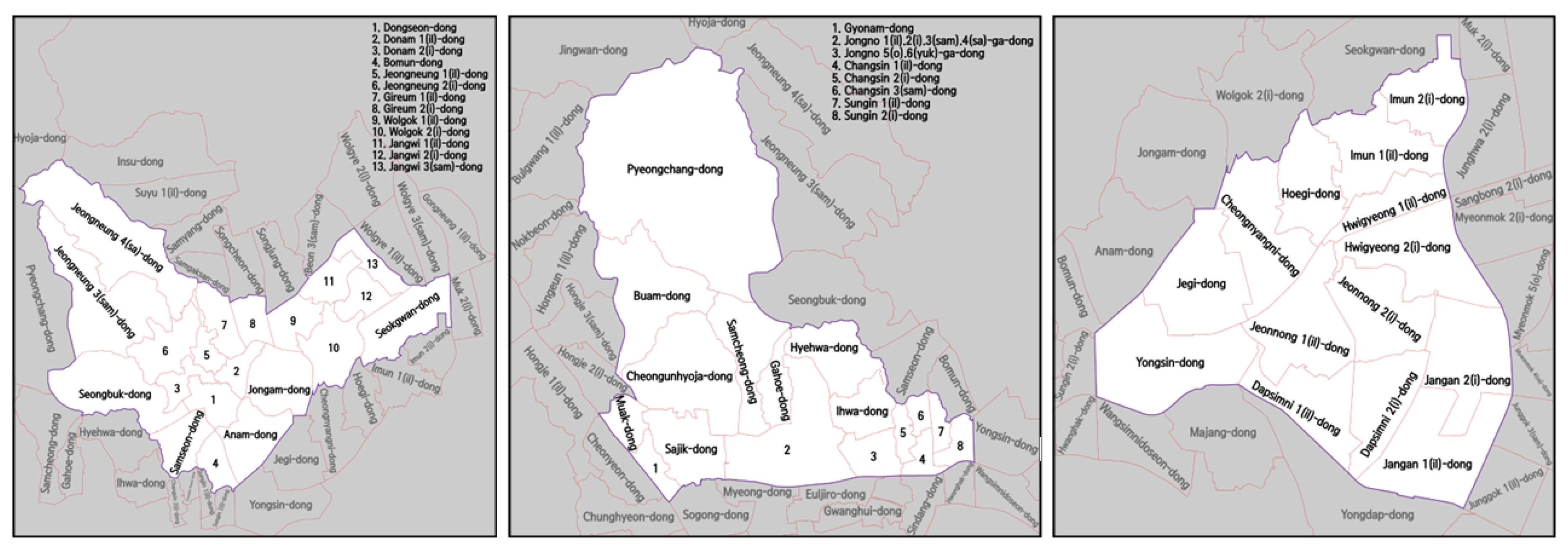
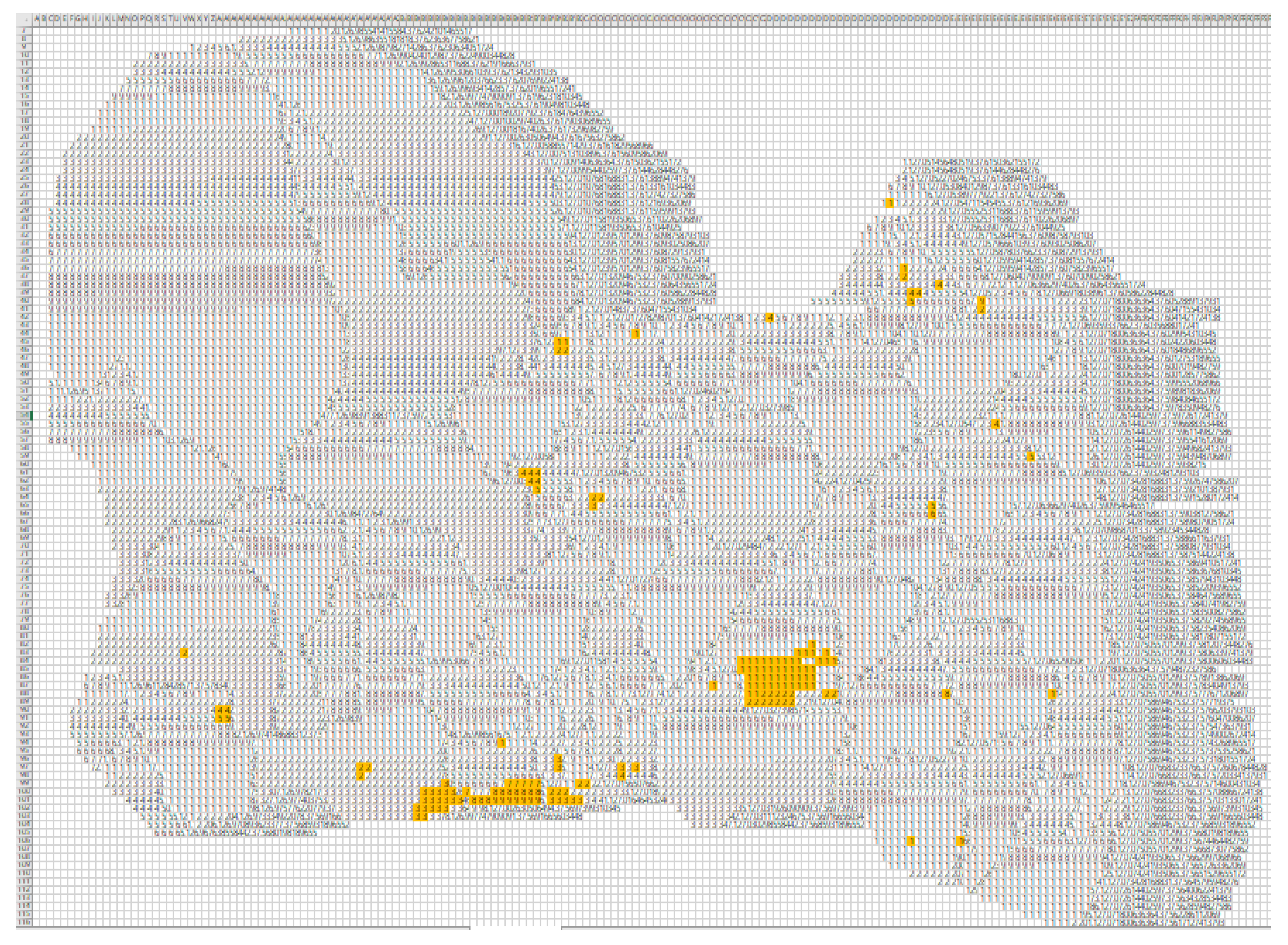
The sub-terminal delivers to three different administrative districts (gu), A, B, and C, as mentioned. The districts can further be divided into 51 smaller administrative units (dong), as shown in Figure 2. The population density of the 51 administrative units was used to probabilistically generate demand. A total of 10,255 cells were created on a spreadsheet to cover the districts, as shown in Figure 3, each cell belonging to one of the 51 units. Once the unit (dong) is chosen by population density, a cell is chosen uniformly within it.
The sub-terminal produces 5250 boxes to be delivered. However, to correlate with the vehicle capacity assumption, 1050 stopping locations, which is one fifth of the demand, are generated. On average, the vehicles will deliver to 1050 stopping locations, of which each location has 5 boxes to be delivered. Among the 1050 stopping locations, traditional markets and apartment complexes account for 5 and 10%, respectively, as shown in Table 1. A total of 1050 stopping locations, including 53 evade market areas, 105 evade apartment complexes, and 892 non-evade areas, were generated.
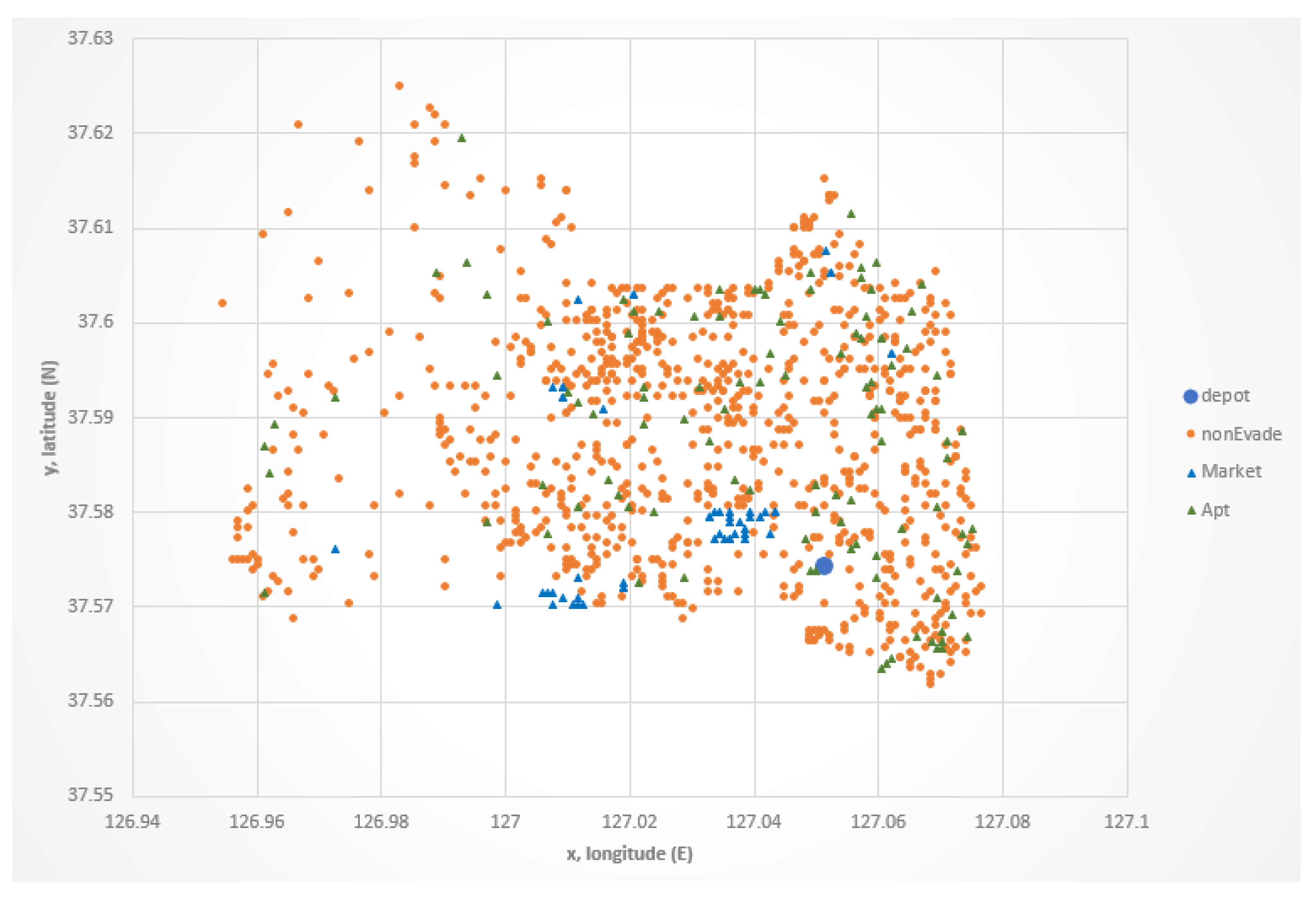
The generation of demands for traditional markets and apartment complexes was carried out as follows. Shown as yellow cells in Figure 3, geographic information for 51 traditional markets in the three districts is used to mark the cells as evade areas. Fifty-three (5% of 1050) yellow cells are randomly chosen to be evade traditional market stopping points. The decisions made by apartment complexes to allow or disallow the entrance of delivery trucks are autonomous to their communities. Their decisions can change at any time. As such, rather than rely on a snap-shot of the current situation, we randomly chose 105 (10% of 1050) non-yellow cells to be evade apartment complex stopping points. Figure 4 shows an example of the generated stopping points. The blue triangles indicate market areas, and the green triangles indicate apartment complexes.
4.1.6. Objective Function
Exact cost information for the company is too sensitive to be revealed. The fuel cost (per km) for the cargo-bike being one unit, we converted all costs into an equivalent unit and approximated the values. Table 2 summarizes the cost information. Truck payments are a daily installment for a purchased vehicle for a five-year period. License plates for trucks must be purchased for business usage. The price for the license plate, insurance premiums, and maintenance costs are also converted into a daily basis. Daily cost items in Table 2 are the fixed costs for each problem set. They are fixed as long as the number of trucks and bikes are determined. On the other hand, labor and fuel costs are variable. With different routings, the total labor and fuel costs change.
The objective function value that needs to be minimized can be expressed as fixed costs plus variable costs. Fixed costs are the daily costs presented in Table 2 multiplied by the number of trucks and bikes. Variable costs are labor costs multiplied by the total time spent, traveling, and delivering, plus fuel costs multiplied by the total distance traveled by the trucks and bikes. The objective function is as follows, and the notations are provided in Table 3 below.
where
4.2. Simulated Annealing (SA)
VRPs are known to be NP-hard [45]. Exact algorithms are adequate for only small problem instances of fewer than 25 customers [46]. A variety of heuristic and meta-heuristic approaches have been applied to the HFVRP, including the iterative local search (ILS) [47,48] and tabu search (TS) [49,50,51]. Again, comprehensive surveys can be found in the literature [2,3]. Simulated annealing (SA), a meta-heuristic method, was used to solve the problems in this paper. The use of SA has been vigorous in the field of VRP research. First introduced by Kirkpatrick et al. [52], SA is a random search algorithm analogous to the annealing process used for metal. In the physical annealing process, a metallic object is heated and slowly cooled. In most cases, the cooling process is sufficiently slow to determine the thermal equilibrium. The higher the temperature, the faster atoms vibrate, enabling them to more easily break linkages and rearrange structures. When objects cool down, atoms eventually create tight bonds or crystalize, and as such, rearrangement trials are repeated countless times to reach equilibrium, i.e., the state of minimal energy. SA mimics this process to find the minimal, or often times maximal, objective function value. The algorithm has proven its value with various optimization problems, including VRP variations. Chiang and Russell [53] applied SA for a time window constrained VRP (TWVRP). Kuo [54] considered a VRP with time-dependent travel speed and proposed an SA-based algorithm to determine the vehicle routing with minimum fuel consumption. This study, on the other hand, aimed to analyze the feasibility and the benefit of the truck–bike mixture model rather than introduce a new methodology to solve an HFVRP.
The algorithm starts with an initial solution, , and initial temperature, . The current temperature, , is updated to after a certain number of perturbation trials. Parameter is a decrement cooling factor usually set between 0.7 and 1. Unlike heuristic algorithms that usually get stuck in a local but not global optimum, SA probabilistically escapes local optima by allowing uphill movements with some probability ), where is the degenerated amount of the objective function value. The probability of accepting a deteriorating configuration comes from Boltzmann’s factor, which indicates the probability of a state of energy, E. The formula implies that if is the same, a higher temperature produces a higher chance of accepting uphill movements, and that if T is the same, a smaller produces a higher chance. This is analogous to the strength of atomic bonds that weakens with higher kinetic energy at higher temperatures. A pseudo code is provided in Algorithm 1.
| Algorithm 1 SA Structure |
| Initialization while > do while IterCount ≤ IterCountMax newSol = SwapTwoNodes(nowSol) if (OFV(newSol) < OFV(bestSol)) bestSol = newSol, IterCount = 0 else IterCount++ if (OFV(newSol) < OFV(nowSol)) = 1.0 else = ()/ if ( > Rand [0, 1]) nowSol = newSol else newSol = nowSol end IterCount = 0 newSol = bestSol nowSol = bestSol = * end |
4.3. Emmisions Calculation
Vehicle carbon emissions stem from a variety of factors, and providing exact calculations is almost impossible. Each country chooses its own calculation method according to its own particular conditions. Mobile combustion is the combustion of fossil fuels that occurs from vehicles such as trucks, buses, and trains, resulting in the emissions of , and so on. Mobile combustion includes the burning of diesel, gasoline, or LPG, and greenhouse gas emissions are calculated by fuel use.
The 2006 IPCC guidelines for national greenhouse gas inventories [55,56] advised governing bodies and researchers to determine calculating methods by considering greenhouse gas inventory constructs, the importance of emission sources in national statistics, and the presence of available data for calculation. It advised using the Tier 3 method when the vehicle kilometers traveled (VKT) by fuel and technology type were available and when country-specific technology-based emission factors were available. When VKT data were available but country-specific emission factors were not, the guidelines advised the use of the Tier 2 (Advanced) method, which uses default, instead of country-specific, factors. Lastly, when neither could be obtained, it advocated the use of the Tier 1 (Simple) method, which calculates greenhouse gas emissions from the total fuel use of road transportation. The present study used the Tier 1 method to calculate greenhouse gas emissions. The emission factors also adhere to the 2006 IPPC suggestions. The guidelines provide a calculation method for CO2 emissions, and another for CH4 and N2O. The estimation of CH4 and N2O is difficult because it depends significantly on emission controls in the fleet or operating characteristics. This paper only estimated carbon emissions by calculating CO2 emissions. Accordingly, calculating CO2 emissions by fuel use produces the following. (Table 4 explains the parameters for the calculation).
All of the carbon in the fuel, including the carbon emitted as CO2, CH4, CO, NMVOC (non-methane volatile organic compound), and PM, is considered in the emission factor [55]. The calculation results show that 1 liter of diesel usage emits 2.57 kg CO2. The 1-ton trucks’ fuel efficiency while delivering is 7.5 km per liter, which produces a value of 0.343 kg CO2 emissions per kilometer. For electricity, 1 kWh of usage emits 0.42 kg CO2. The e-bikes can travel a total of 50 km using 1 kWh of electricity, which equates to 0.0084 kg CO2 emissions per kilometer.
5. Computational Results and Comparison
5.1. Number of Trucks and Bikes
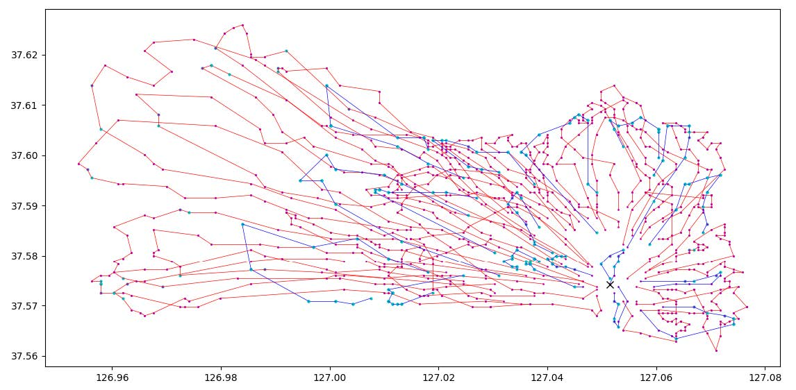
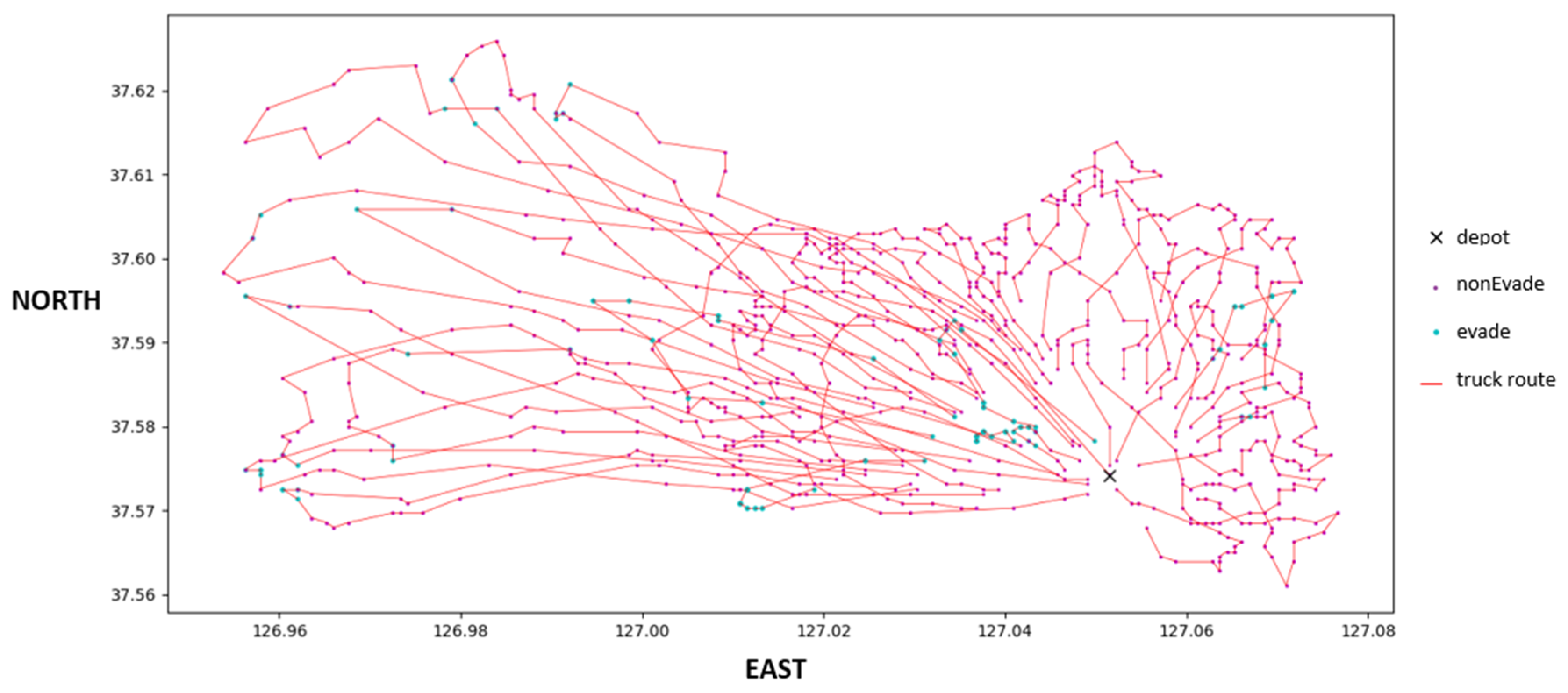
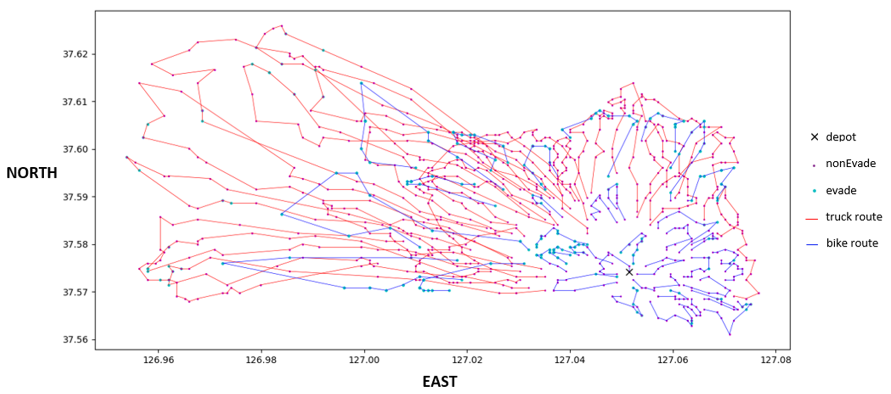
As mentioned in Section 4.1.2, trucks are replaced in two-truck intervals to determine the ratio in which costs are minimized. Please note that only an even number of trucks are replaced because 1.5 bikes are required to replace one truck, and thus, an odd replacement number would always produce redundancies. The experiment was carried out on Java with an Intel(R) Core (TM) i5-2500U CPU @ 2.20 GHz. The simulated annealing initial temperature, , and final temperature, , were set to 1000 and 0.1, respectively. The cooling rate was set to 0.95, and for each temperature, (number of truck routes + bike routes) 50,000 iterations were made to search for a solution. Demand was generated five times. For each demand and replacement number, 30 replications were made and averaged. Some solution examples are provided in Figure 5, Figure 6 and Figure 7. In the figures, the X and Y axes are the geographic coordinates of the stopping locations, e.g., 127.00 East and 37.60 North. The blue and red dots indicate evade and non-evade areas, respectively. The red lines are truck routes, and the blue lines are e-bike routes.
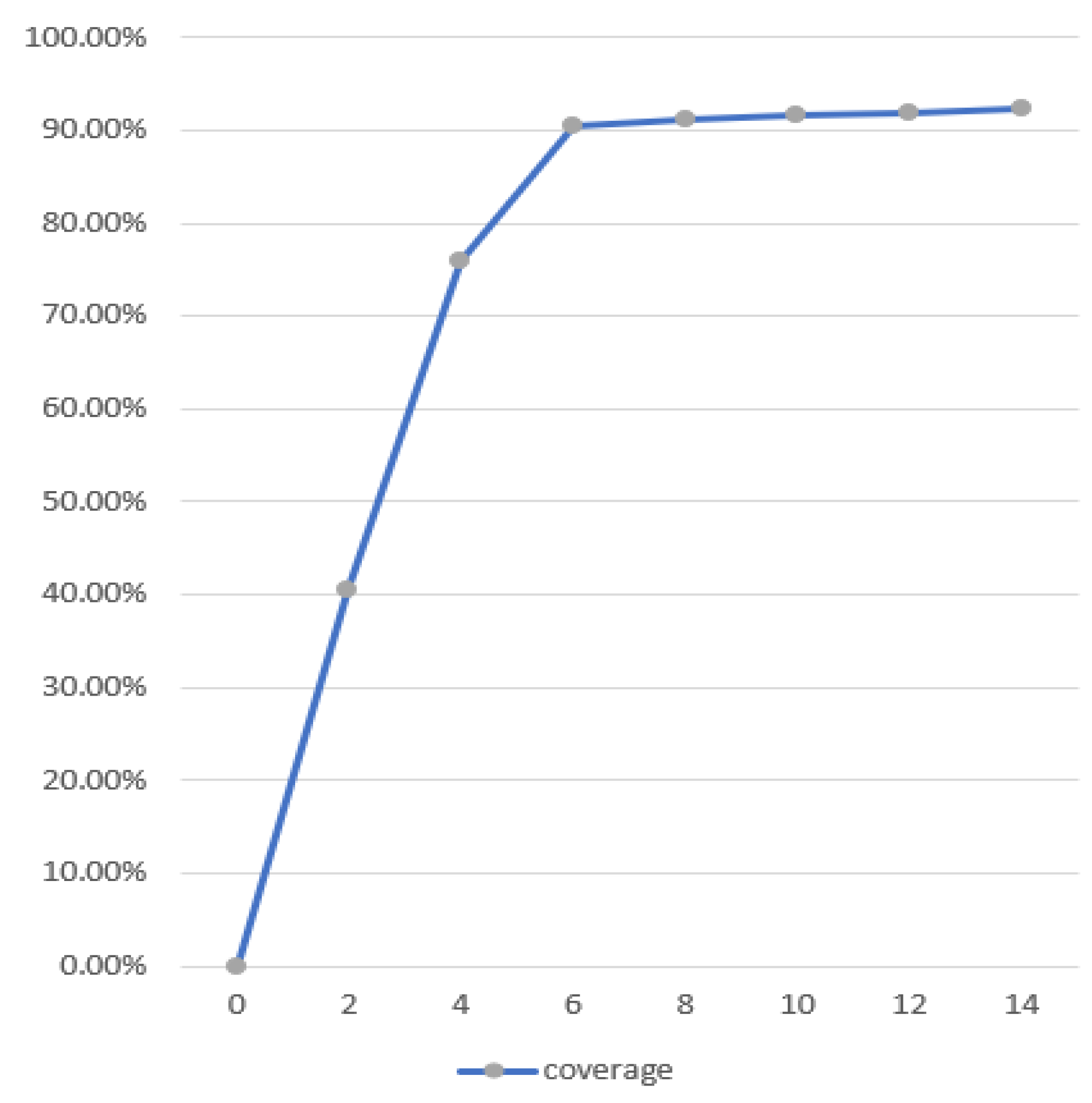
Table 5 summarizes the results. Figure 8 presents four lines indicating fixed costs, fuel costs, labor costs, and total costs. The latter is the sum of the fixed and variable costs (fuel and labor costs). We concluded that costs are minimized when six trucks are replaced with nine bikes. The benefit of replacement comes from (i) the reduced fixed costs, (ii) the reduced fuel costs, and (iii) the reduced labor costs. The most dominant among them is the reduced labor costs. As bikes take over evade areas, labor costs decrease accordingly. The Bike (%) in Table 5 and Figure 9 shows the percentage of evade areas covered by bikes. Bike coverage increases from zero to 14 replacements, but after six replacements, the increment becomes insignificant. More bike replacements after six do not really increase bike coverage. This increases travel time (labor costs), which is more significant than the decreased fuel costs.
5.2. Scenarios and CO2 Emmisions
The real world is not static but rather dynamic. Verifying only the averaged situation, which has a 15% evade rate and a demand of 5250 boxes, might result in a generalization fallacy. To see the true effectiveness of the mixture model, we need to embrace some of the sensitivities of the world. We did this by exploring several scenarios with two axes, the first being the evade rate. The average evade rate is about 15%, but this can change daily. We set three gradations on the axis—10, 15, and 20%. The other axis is the demand, the number of boxes to be delivered, naturally translating into the number of stopping points. Demand for the day always changes, so we applied five gradations on the axis. The average is 0%, and the gradations were set at –20%, –10%, 0%, +10%, and +20%. With these two criteria, we had 15 possible scenarios and can see the varying cost effects of the mixture model. Demand was generated five times for each scenario. For each generated demand, 10 replications were made and averaged.
Figure 10 and Table 6 summarize the cost reduction results. The dotted and solid lines in Figure 10 indicate the truck-only and the truck–bike mixture model, respectively. For the averaged scenario where the evade rate is 15% and the demand is +0%, a 14.1% cost reduction was observed. The cost reduction rate varied from one scenario to another. A minimum of 5.7% and maximum of 26.9% in cost reduction was observed.
In addition, carbon emission reductions are also of great interest in this study. Assuming 310 operating days a year, yearly carbon emissions were calculated using the method explained in Section 4.3. The differences between the two models on the scenarios are shown in Table 7. We see an approximate 10% reduction in carbon emissions. However, there were no observed tendencies correlating to changes in the evade rate or demand quantity. This can be explained in the way that fuel costs affect total costs. As can be seen in Figure 8, fuel costs have the smallest effect on total costs. On the other hand, labor costs have the greatest impact. When routes are being constructed to minimize costs, fuel is not the main concern. In other words, reducing the distance traveled by trucks and increasing the distance traveled by bikes results in a small decrease in fuel costs but much greater increase in labor costs. We therefore concluded that it is reasonable for carbon reductions to not have direct correlations across different scenarios.
6. Discussion and Conclusions
In South Korea, delivery trucks are unable to access certain off-limits (evade) areas, and this results in additional time costs. Numerous studies, both domestically in Korea and abroad, have explored the notion of replacing delivery trucks with other transportation modes, one possibility being electric cargo-bikes. The present study has explored this latter possibility and verified a number of potential benefits. In particular, we considered employing the one of the most popular e-bike models, and we then relied on the existing literature to build our assumptions. The VRP and HFVRP were solved using the simulated annealing algorithm for the truck-only and truck–bike mixture models, respectively. The results were used to verify the economic viability of the proposed model and analyze the effects in terms of reducing carbon emissions.
The study used data provided by one of the three major courier service companies in South Korea. One of the company’s depots, or terminals, serves three administrative districts, delivering 5250 boxes daily. We empirically determined the appropriate ratio of trucks to bikes by solving the HFVRP while replacing trucks with bikes from two to many. In this case, the ratio of 29 to nine was found to be optimal. The results showed that after replacing six trucks, further replacements would yield inefficiencies.
Using the 29-to-nine ratio, but also embracing a healthy dose of reality, we established 15 scenarios and observed the varying effects. We compared the operating costs and carbon emissions of the truck-only and truck–bike mixture models. The experimental results showed that cost reductions were expected to be 14.1% for the average scenario. A total of 5.7% and 26.9% cost reductions were seen, respectively, for the scenario where the demand quantity and evade rate were the lowest, and for the antipodal scenario. Higher evade rates and higher demand yielded higher cost reductions. From a sustainability standpoint, carbon emission reductions were expected to be around 10%, with no clear tendencies regarding changes in the demand quantity or evade rate. This lack of tendencies resulted from the insignificant impact of fuel costs on the total operating costs.
The major assumptions used in this study (e.g., assumptions regarding travel speed or delivery time) will vary in reality. Likewise, the appropriate truck-to-bike ratio was determined for this case only and is subject to variations based on circumstances. However, if the evade areas are still present, we believe that in most cases, our approach will produce a convex–downward cost curve when replacing trucks with bikes one by one.
The experiment revealed that labor costs dominated the total costs. Like any other last mile logistics operations, managerial issues revolved around the labor costs. The location of the sub-terminal had to be determined taking various factors into account, including evade areas and their cost. Taking evade areas into consideration, the optimal location might shift. Further, having the right capacity at the sub-terminal, where redundancies and overtime would strike a balance, would be critical in reducing labor costs. The implementation of advanced IT systems to support vehicle routing or resource management could also lower costs. Moreover, labor costs might be further reduced if the government aided silver (senior) citizen workers for deliveries.
Recently in South Korea, much attention has been placed on arguments between courier service companies and certain apartment complex representatives who have refused to permit delivery trucks to enter the property. Compromises could be reached if bikes were used for those areas. Particulate matter (PM), or fine dust, is another serious issue. The truck–bike mixture model naturally reduces PM emissions as well as carbon emissions. The truck-bike mixture would also encourage brand loyalty from environmentally sensitive customers. Finally, the use of cargo-bikes would also help to reduce traffic congestion and other traffic issues such as blockages that occur when multiple delivery trucks are forced to park outside of apartment complexes and markets.
An additional concern is the emission of non-carbon pollutants, such as SO2 and PM. The proposed model naturally reduces PM emissions, but specific measures and the calculation of emissions could be meaningful and are an intriguing future research direction.
Author Contributions
Conceptualization, J.C.; Methodology, K.L.; Software, K.L.; Validation, K.L., J.C. and J.K.; Formal Analysis, K.L.; Resources, J.K.; Data Curation, K.L.; Writing—Original Draft Preparation, K.L.; Writing—Review and Editing, J.C.; Visualization, K.L.; Supervision, J.C.; Project Administration, J.C.
Funding
This work was partially supported by Jungseok Logistics Foundation Grant.
Acknowledgments
Thanks to C. Kim and Y. Cho in Hanjin Transportation Co., LTD. for their data supports.
Conflicts of Interest
The authors declare no conflict of interest.
References
- Greenhouse Gas Inventory & Research Center of Korea (GIR). 2017 National Greenhouse Gas Inventory Report; Greenhouse Gas Inventory & Research Center: Seoul, Korea, 2017.
- Eksioglu, B.; Vural, A.V.; Reisman, A. The vehicle routing problem: A taxonomic review. Comput. Ind. Eng. 2009, 57, 1472–1483. [Google Scholar] [CrossRef]
- Braekers, K.; Ramaekers, K.; Van Nieuwenhuyse, I. The vehicle routing problem: State of the art classification and review. Comput. Ind. Eng. 2016, 99, 300–313. [Google Scholar] [CrossRef]
- Park, Y.; Chae, J. A review of the solution approaches used in recent G-VRP (Green Vehicle Routing Problem). Int. J. Adv. Logist. 2014, 3, 27–37. [Google Scholar] [CrossRef]
- Ranieri, L.; Digiesi, S.; Silvestri, B.; Roccotelli, M. A review of last mile logistics innovations in an externalities cost reduction vision. Sustainability 2018, 10, 782. [Google Scholar] [CrossRef]
- Bányai, T. Real-time decision making in first mile and last mile logistics: How smart scheduling affects energy efficiency of hyperconnected supply chain solutions. Energies 2018, 11, 1833. [Google Scholar] [CrossRef]
- Giaglis, G.M.; Minis, I.; Tatarakis, A.; Zeimpekis, V. Minimizing logistics risk through real-time vehicle routing and mobile technologies: Research to date and future trends. Int. J. Phys. Distrib. Logist. Manag. 2004, 34, 749–764. [Google Scholar] [CrossRef]
- Taillard, E.D. A heuristic column generation method for the heterogeneous fleet VRP. RAIRO Oper. Res. 1999, 33, 1–14. [Google Scholar] [CrossRef] [Green Version]
- Hoff, A.; Andersson, H.; Christiansen, M.; Hasle, G.; Løkketangen, A. Industrial aspects and literature survey: Fleet composition and routing. Comput. Oper. Res. 2010, 37, 2041–2061. [Google Scholar] [CrossRef] [Green Version]
- Korean Ministry of Environment. Post-2020 Greenhouse Gas Emissions Reduction Targets and Implementation Plans; Korean Ministry of Environment: Sejong, Korea, 2015.
- Korean Ministry of Land, Infrastructure, and Transport. National Transportation Statistics 2015; Korean Ministry of Land, Infrastructure, and Transport: Sejong, Korea, 2015.
- Poudenx, P. The effect of transportation policies on energy consumption and greenhouse gas emission from urban passenger transportation. Transp. Res. Part A Policy Pract. 2008, 42, 901–909. [Google Scholar] [CrossRef]
- Schwanen, T.; Banister, D.; Anable, J. Scientific research about climate change mitigation in transport: A critical review. Transp. Res. Part A Policy Pract. 2011, 45, 993–1006. [Google Scholar] [CrossRef] [Green Version]
- Yang, C.; McCollum, D.; McCarthy, R.; Leighty, W. Meeting an 80% reduction in greenhouse gas emissions from transportation by 2050: A case study in California. Transp. Res. Part D Transp. Environ. 2009, 14, 147–156. [Google Scholar] [CrossRef] [Green Version]
- Greene, D.L.; Plotkin, S. Reducing Greenhouse Gas Emission from US Transportation. Available online: https://rosap.ntl.bts.gov/view/dot/23588 (accessed on 20 February 2019).
- Stanley, J.K.; Hensher, D.A.; Loader, C. Road transport and climate change: Stepping off the greenhouse gas. Transp. Res. Part A Policy Pract. 2011, 45, 1020–1030. [Google Scholar] [CrossRef]
- Hickman, R.; Ashiru, O.; Banister, D. Transport and climate change: Simulating the options for carbon reduction in London. Transp. Policy 2010, 17, 110–125. [Google Scholar] [CrossRef]
- Timilsina, G.R.; Shrestha, A. Transport sector CO2 emissions growth in Asia: Underlying factors and policy options. Energy Policy 2009, 37, 4523–4539. [Google Scholar] [CrossRef]
- Ang-Olson, J.; Schroeer, W. Energy efficiency strategies for freight trucking potential impact on fuel use and greenhouse gas emissions. Transp. Res. Rec. 2002, 11–18. [Google Scholar] [CrossRef]
- Kamakaté, F.; Schipper, L. Trends in truck freight energy use and carbon emissions in selected OECD countries from 1973 to 2005. Energy Policy 2009, 37, 3743–3751. [Google Scholar] [CrossRef]
- Eom, J.; Schipper, L.; Thompson, L. We keep on truckin’: Trends in freight energy use and carbon emissions in 11 IEA countries. Energy Policy 2012, 45, 327–341. [Google Scholar] [CrossRef]
- Li, H.; Lu, Y.; Zhang, J.; Wang, T. Trends in road freight transportation carbon dioxide emissions and policies in China. Energy Policy 2013, 57, 99–106. [Google Scholar] [CrossRef]
- Zanni, A.M.; Bristow, A.L. Emissions of CO2 from road freight transport in London: Trends and policies for long run reductions. Energy Policy 2010, 38, 1774–1786. [Google Scholar] [CrossRef]
- Léonardi, J.; Baumgartner, M. CO2 efficiency in road freight transportation: Status quo, measures and potential. Transp. Res. Part D Transp. Environ. 2004, 9, 451–464. [Google Scholar] [CrossRef]
- Lee, D.Y.; Thomas, V.M.; Brown, M.A. Electric urban delivery trucks: Energy use, greenhouse gas emissions, and cost-effectiveness. Environ. Sci. Technol. 2013, 47, 8022–8030. [Google Scholar] [CrossRef] [PubMed]
- Barnitt, R. FedEx Express Gasoline Hybrid Electric Delivery Truck Evaluation: 12-Month Report, Technical Report; NREL: Golden, CO, USA, 2011. [Google Scholar]
- Kim, N.S.; Van Wee, B. Toward a better methodology for assessing CO2 emissions for intermodal and truck-only freight systems: A European case study. Int. J. Sustain. Transp. 2014, 8, 177–201. [Google Scholar] [CrossRef]
- Kim, N.S.; Van Wee, B. Assessment of CO2 emissions for truck-only and rail-based intermodal freight systems in Europe. Transp. Plan. Technol. 2009, 32, 313–333. [Google Scholar] [CrossRef]
- Hong, Z.; Zhiliang, W.; Wei, L. Bicycle-based courier and delivery services in Beijing: Market analysis. Transp. Res. Rec. J. Transp. Res. Board 2006, 1954, 45–51. [Google Scholar] [CrossRef]
- Schier, M.; Offermann, B.; Weigl, J.D.; Maag, T.; Mayer, B.; Rudolph, C.; Gruber, J. Innovative two wheeler technologies for future mobility concepts. In Proceedings of the 11th Intertnational Conference on Ecological Vehicles and Renewable Energies (EVER 2016), Monte Carlo, Monaco, 6–8 April 2016. [Google Scholar] [CrossRef]
- Gruber, J.; Ehrler, V.; Lenz, B. Technical potential and user requirements for the implementation of electric cargo bikes in courier logistics services. In Proceedings of the 13th World Conference on Transport Research (WCTR), Rio de Janeiro, Brazil, 15–17 July 2013; pp. 1–16. [Google Scholar]
- Gruber, J.; Kihm, A.; Lenz, B. A new vehicle for urban freight? An ex-ante evaluation of electric cargo bikes in courier services. Res. Transp. Bus. Manag. 2014, 11, 53–62. [Google Scholar] [CrossRef] [Green Version]
- Choubassi, C.; Seedah, D.P.K.; Jiang, N.; Walton, C.M. Economic analysis of cargo cycles for urban mail delivery. Transp. Res. Rec. J. Transp. Res. Board 2016, 2547, 102–110. [Google Scholar] [CrossRef]
- Rudolph, C.; Gruber, J. Cargo cycles in commercial transport: Potentials, constraints, and recommendations. Res. Transp. Bus. Manag. 2017, 24, 26–36. [Google Scholar] [CrossRef]
- Tipagornwong, C.; Figliozzi, M. Analysis of competitiveness of freight tricycle delivery services in urban areas. Transp. Res. Rec. J. Transp. Res. Board 2014, 2410, 76–84. [Google Scholar] [CrossRef]
- Cherry, C.R.; Weinert, J.X.; Xinmiao, Y. Comparative environmental impacts of electric bikes in China. Transp. Res. Part D Transp. Environ. 2009, 14, 281–290. [Google Scholar] [CrossRef] [Green Version]
- Cherry, C.R. Electric Two-Wheelers in China: Analysis of Environmental, Safety, and Mobility Impacts; University of California: Berkeley, CA, USA, 2007. [Google Scholar]
- Cherry, C.; Weinert, J.; Ma, C. The Environmental Impacts of Electric Bikes in Chinese Cities; US Berkley Center for Future Urban Transport: Berkeley, CA, USA, 2007. [Google Scholar]
- Cherry, C. Electric Bike Use in China and Their Impacts on the Environment, Safety, Mobility and Accessibility; UC Berkeley Center for Future Urban Transport, A Volvo Center of Excellence: Berkley, CA, USA, 2007. [Google Scholar]
- Lenz, B.; Riehle, E. Bikes for Urban Freight? Transp. Res. Rec. J. Transp. Res. Board 2013, 2379, 39–45. [Google Scholar] [CrossRef]
- Wrighton, S.; Reiter, K. CycleLogistics—Moving Europe forward! Transp. Res. Proced. 2016, 12, 950–958. [Google Scholar] [CrossRef]
- Nocerino, R.; Colorni, A.; Lia, F.; Luè, A. E-bikes and E-scooters for smart logistics: Environmental and economic sustainability in Pro-E-bike Italian pilots. Transp. Res. Proced. 2016, 14, 2362–2371. [Google Scholar] [CrossRef]
- Lia, F.; Nocerino, R.; Bresciani, C.; Colorni, A.; Luè, A. Promotion of E-bikes for delivery of goods in European urban areas: An Italian case study. Transp. Res. Proced. 2014, 14, 2362–2371. [Google Scholar]
- Conway, A.; Cheng, J.; Kamga, C.; Wan, D. Cargo cycles for local delivery in New York City: Performance and impacts. Res. Transp. Bus. Manag. 2017, 24, 90–100. [Google Scholar] [CrossRef]
- Lenstra, J.K.; Rinnooy-Kan, A.H.G. Complexity of vehicle routing and scheduling problems. Networks 1979, 11, 221–227. [Google Scholar] [CrossRef]
- Fisher, L. Optimal solution of vehicle routing problems K-trees. Oper. Res. 2013, 42, 626–642. [Google Scholar] [CrossRef]
- Subramanian, A.; Huachi, P.; Penna, V.; Uchoa, E.; Satoru, L. Discrete optimization. A hybrid algorithm for the heterogeneous fleet vehicle routing problem. Eur. J. Oper. Res. 2012, 221, 285–295. [Google Scholar] [CrossRef]
- Huachi, P.; Penna, V.; Subramanian, A. An iterated local search heuristic for the heterogeneous fleet vehicle routing problem. J. Heuristics 2013, 19, 201–232. [Google Scholar] [CrossRef]
- Gendreau, M.; Laporte, G.; Musaraganyi, C.; Taillard, D.D. A tabu search heuristic for the heterogeneous fleet vehicle routing problem. Comput. Oper. Res. 1999, 26, 1153–1173. [Google Scholar] [CrossRef]
- Prastacos, D.C. A reactive variable neighborhood tabu search for the heterogeneous fleet vehicle routing problem with time windows. J. Heuristics 2008, 14, 425–455. [Google Scholar] [CrossRef]
- Brandao, J. A tabu search algorithm for the heterogeneous fixed fleet vehicle routing problem. Comput. Oper. Res. 2011, 38, 140–151. [Google Scholar] [CrossRef]
- Kirkpatrick, S.; Gelatt, C.D., Jr.; Vecchi, M.P. Optimization by simulated annealing. Science 1983, 220, 671–680. [Google Scholar] [CrossRef] [PubMed]
- Chiang, W.-C.; Russell, R.A. Simulated annealing metaheuristics for the vehicle routing problem with time windows. Ann. Oper. Res. 1996, 63, 3–27. [Google Scholar] [CrossRef]
- Kuo, Y. Using simulated annealing to minimize fuel consumption for the time-dependent vehicle routing problem. Comput. Ind. Eng. 2010, 59, 157–165. [Google Scholar] [CrossRef]
- Waldron, C.D.; Harnisch, J.; Lucon, O.; Mckibbon, R.S.; Saile, S.B.; Wagner, F.; Walsh, M.P.; Maurice, L.Q.; Hockstad, L.; Höhne, N.; et al. 2006 IPCC Guidelines for National Greenhouse Gas Inventories; IPCC: Geneva, Switzerland, 2006; Chapter 3, Mobile Combustion; Volume 2. [Google Scholar]
- Penman, J.; Gytarsky, M.; Hiraishi, T.; Irving, W.; Krug, T. 2006 IPCC Guidelines for National Greenhouse Gas Inventories, Overview; IPCC: Geneva, Switzerland, 2006; 12p. [Google Scholar]
Figure 1.
A brief map of Seoul and the three districts (red-shaded).

Figure 2.
Administrative units, A, B, and C in order.

Figure 3.
Cells created to map the three districts (Yellow cells are market areas).

Figure 4.
Example of generated demand.

Figure 5.
Solution example with 35 trucks.

Figure 6.
Solution example with 29 trucks and 9 bikes.

Figure 7.
Solution example with 23 trucks and 15 bikes.

Figure 8.
Result of replacing trucks with bikes.

Figure 9.
% of evade areas covered by bikes.

Figure 10.
Results of 15 scenarios on costs for the truck-only model and truck–bike mixture model.


Table 1.
Data and information for the sub-terminal.
| Number of Trucks | Average Cargo Quantities (Day, Box) | Amount of Fuel Usage (Day, L) | Number of Delivery Points | Apartment Complexes | Conventional Markets |
|---|---|---|---|---|---|
| 35 | 5253.5 | 385 L | 1000 | 10% | 5% |
Table 2.
Cost comparison of truck and electric bike.
| Vehicle | Car Payment (Day) | License Plate (Day) | Vehicle Insurance (Day) | Cargo Insurance (Day) | Maintenance (Day) | Labor (Hour) | Fuel Cost (km) | |
|---|---|---|---|---|---|---|---|---|
| Regular | Overtime | |||||||
| Truck | 2508 | 3343 | 1634 | 192 | 2034 | 6101 | 9152 | 114 |
| E-Bike | 1672 | 0 | 1089 | 128 | 1356 | 6101 | 9152 | 1 |
Table 3.
Parameters of truck and electric bicycle.
| Parameter | Notation |
|---|---|
| Daily car payment for truck , for bike | |
| Daily license plate for truck , for bike | |
| Daily vehicle insurance for truck , for bike | |
| Daily cargo insurance for truck , for bike | |
| Daily maintenance for truck , for bike | |
| Number of routes for trucks | |
| Number of routes for bikes | |
| Hourly regular labor cost | |
| Hourly overtime labor cost | |
| Standard working hours (daily), 9 hours in this case | |
| Fuel cost per km for truck , for bike | |
| Distance traveled by trucks | |
| Distance traveled by bikes | |
| Time spent by trucks | |
| Time spent by bikes |
Table 4.
Parameters for greenhouse gas emission calculation.
| Parameter | Notation |
|---|---|
| Greenhouse gas emission by fuel consumption | |
| Fuel consumption () | |
| Caloric value liquid (), gas () | |
| Conversion factor (1TJ = ) | |
| Greenhouse gas emission factor, in fuels suggested by the IPPC |
Table 5.
Result of replacing trucks with bikes on cost.
| Replace | 0 | 2 | 4 | 6 | 8 | 10 | 12 | 14 | 16 | 18 | 20 |
|---|---|---|---|---|---|---|---|---|---|---|---|
| Fixed cost | 557,025 | 546,066 | 535,107 | 524,148 | 513,189 | 502,230 | 491,271 | 480,312 | 469,353 | 458,394 | 447,435 |
| Variable cost | 3,694,092 | 3,310,938 | 3,142,052 | 3,100,874 | 3,115,666 | 3,137,310 | 3,162,776 | 3,190,980 | 3,224,267 | 3,259,886 | 3,301,762 |
| Total cost | 4,251,117 | 3,857,004 | 3,677,159 | 3,625,022 | 3,628,855 | 3,639,540 | 3,654,047 | 3,671,292 | 3,693,620 | 3,718,280 | 3,749,197 |
| Bike (%) | 0.00% | 50.59% | 75.95% | 90.51% | 90.51% | 90.61% | 90.61% | 90.63% | 90.65% | 90.65% | 90.72% |
Table 6.
Cost reduction from the truck-only model to the truck–bike mixture model.
| Evade Area Rate | 10% | 15% | 20% |
|---|---|---|---|
| Demand +20% | 17.1% | 23.2% | 26.9% |
| Demand +10% | 14.4% | 18.2% | 18.9% |
| Demand 0% | 7.7% | 14.1% | 21.1% |
| Demand −10% | 6.3% | 9.3% | 12.4% |
| Demand −20% | 5.7% | 8.6% | 10.8% |
Table 7.
Carbon reduction from the truck-only model to the truck–bike mixture model.
| Evade Area Rate | 10% | 15% | 20% |
|---|---|---|---|
| Demand +20% | 6535 kgCO2 (11.2%) | 6139 kgCO2 (10.6%) | 5221 kgCO2 (9.1%) |
| Demand +10% | 5922 kgCO2 (10.4%) | 6054 kgCO2 (10.7%) | 5161 kgCO2 (9.1%) |
| Demand 0% | 3587 kgCO2 (6.6%) | 6148 kgCO2 (11.0%) | 3882 kgCO2 (7.1%) |
| Demand −10% | 5404 kgCO2 (10.1%) | 6418 kgCO2 (11.9%) | 8097 kgCO2 (14.4%) |
| Demand −20% | 4968 kgCO2 (9.7%) | 5635 kgCO2 (10.9%) | 5574 kgCO2 (10.9%) |
© 2019 by the authors. Licensee MDPI, Basel, Switzerland. This article is an open access article distributed under the terms and conditions of the Creative Commons Attribution (CC BY) license (http://creativecommons.org/licenses/by/4.0/).
Share and Cite
MDPI and ACS Style
Lee, K.; Chae, J.; Kim, J. A Courier Service with Electric Bicycles in an Urban Area: The Case in Seoul. Sustainability 2019, 11, 1255. https://doi.org/10.3390/su11051255
AMA Style
Lee K, Chae J, Kim J. A Courier Service with Electric Bicycles in an Urban Area: The Case in Seoul. Sustainability. 2019; 11(5):1255. https://doi.org/10.3390/su11051255
Chicago/Turabian StyleLee, Keyju, Junjae Chae, and Jinwoo Kim. 2019. "A Courier Service with Electric Bicycles in an Urban Area: The Case in Seoul" Sustainability 11, no. 5: 1255. https://doi.org/10.3390/su11051255
Note that from the first issue of 2016, this journal uses article numbers instead of page numbers. See further details here.