Performance Analysis and Improvement of the Bike Sharing System Using Closed Queuing Networks with Blocking Mechanism

Abstract

The Bike Sharing System is a sustainable urban transport solution that consists of a fleet of bikes placed in various stations. Users will be satisfied if they find available bikes at their departure station and free docks at the destination. Despite the regulation operations of the system provider (i.e., redistribution of bikes by truck) deeper modifications (bike fleet size or station capacity) are often necessary to ensure a satisfactory service rate. In this paper, we model a sub-graph of a Bike Sharing System using the closed queuing network with a Repetitive-Service-Random-Destination blocking mechanism. This model is solved using the Maximum Entropy Method. This model faithfully reproduces the system dynamics considering the limited capacity of stations. We analyze the performance, particularly, via an overall performance indicator of the system. The various control and monitoring decisions (fleet-size, capacity of stations, incoming and outgoing flow of bikes) are applied to find out the best performance levels. The results demonstrate that the overall performance is robust enough regarding the fleet size changes but it degrades with the increase of the stations’ capacity. Finally, the arrival and departure flows control is an efficient and powerful operational leverage.

1. Introduction

Since its first implementation in Amsterdam in 1965 [1], the Bike Sharing Systems (BSS) has considerably evolved. Such systems offer a flexible mode of transportation and can help reduce congestion. These systems support the mitigation of climate change by putting forward the sustainabality of transportation.

There are mainly two types of BSS. The first one, studied in this paper, consists of the stations located throughout the city. Every station has a limited number of docking spaces. The user picks up a bike from a non-empty station, uses it and brings it to a destination station if a free dock is available. Otherwise, he/she goes to another station for docking. The major concern in such a system is to determine the appropriate number of bikes and docks per station [2,3] that could ensure the highest satisfaction rate. The second type of BSS is the newest generation of BSS. This system provides dockless bikes that do not require stations to sign in or sign out from the system. The bikes are placed everywhere and they are geographically tracked using a Global Positioning System [4].

Relevant strategies for bike redistribution, fleet-sizing, station docking capacity and geographic dispatching of stations are among the most studied operations in this field.

Three sets of operations can be carried out to increase the BSS performances:

• Monitoring. The monitoring operations are real-time or short time regulation activities aiming to empty docks in the saturated stations and feeding the empty ones by relocating the bikes using trucks [5,6]. Alternatively, the operator offers financial incentives to the users, who then relocate the bikes themselves [7,8,9].
• Controlling. Controlling means modifying the number of docks and bikes of the BSS. These actions are more expensive and often require transformations in the stations and in their control system [10,11].
• (Re)-Designing. Design consists in designing the initial bike network. Redesign consists in partially or totally redefining the system by adding new stations or removing useless stations. Redesigning implies making decisions on a wider scale about the station capacity and the fleet size [12,13].

The activities of Monitoring, Control and Re-design are performed by the BSS operator. A rational way to make the right and relevant decisions is to assess their consequences using a realistic BSS model before any real implementation. Such modeling has to deal with (i) stochastic parameters and (ii) scaling. Scaling means being able to model a BSS according to several levels of detail. It also means dealing with the size of the BSS.

Various modeling techniques have been developed and tested for relevance and predictability. Hereafter, we discuss the related works in the BSS monitoring-control-design to show what challenges still persist and to clarify our motivations. A BSS is a stochastic system. Parameters such as the inter-arrivals of the users or the trip times are random [14,15]. The stochastic models permit a transient and steady-state evaluation of such systems. Some research works use a discrete event simulation or some formal models based on the stochastic techniques. Here, the state of the art focuses on these works excluding the other techniques such as data mining [16,17,18] or mathematical programming [19,20,21].

The simulation works are used for BSS studies or more generally for Vehicle Sharing Systems, noted VSS [22,23,24,25,26,27,28]. The main approach is the following: first, the model’s components (users, bikes, stations) and their parameters are identified. Then, the dynamic behavior of each component is programmed using the possibilities offered by the simulation environment. Running a discrete event simulation is based on the sequential execution of the elementary events ordered in sample paths [29]. The elementary events can be, for instance, the arrival to or the departure from the bike stations. Numerous sample paths are generated to characterize the behavior patterns. The system state evolves after the occurrence or activation of the elementary events contained in those sample paths. At the end of the simulation, the pre-selected performance indicators and the behaviors of various components are studied based on the collected data. The goals of simulation studies are context-specific (vehicles usage rate or users’ waiting time) or generic (profit or service rate improvement). For instance, in [22], the authors use a simulation model for the relocation of vehicles (i.e., voluntary displacement of vehicles) to increase the system revenue and raise the level of the service defined as “the ratio of the average number of served users to the total number of users arriving at the station”.

Among the stochastic techniques, the Closed Queueing Network (CQN) fits well to the VSS studies because of the fixed number of jobs (i.e., vehicles). Between all types of CQN, the BCMP (Baskett, Chandy, Muntz & Palacios) [30] are the most often used for modeling the VSS. A BCMP-Queueing Network is an extension of the Jackson network. The BCMP is charecterized by a product form solution for the joint distribution of the jobs in the network in the steady-state. This formulation makes the evaluation of the state-probabilities much easier by allowing to study each bike station independently from the other even if they belong to a closed network. George and Xia [31] were the first to use the BCMP-Queueing Network model for VSS. In this model, a bike station is considered as a single server queuing system with a queue of bikes waiting for service. Service time is the time between the arrival of two users to pick up a bike. The travel between two bike stations is modeled by a queue with an infinite server. George and Xia [31] look for the optimal fleet size and propose a nonlinear optimization problem by defining the profit of the operator as a function of the fleet size. Authors prove that the stations should have the same availabilities to meet maximum user satisfaction and they solve the CQN problem with a system of 100 stations. Fanti et al. in [32] model an electrical VSS to evaluate the operator revenue. They extend the framework introduced by George and Xia [31] by adding multiple servers queues to illustrate the recharging process.

The limitation of these author’s works are due to the fact that they consider that the stations have an unlimited capacity. Some other works [33,34,35] model the system using aggregation manner assuming that all the stations of the VSS belong to only one cluster called a homogeneous system. This model presupposes that stations have the same static and dynamic parameters (i.e., station capacities, arrival rate of users, routing between the stations). These hypotheses are used to study large systems and assess the asymptotic performances. However, a real VSS contains highly dynamic stations (e.g., the stations close to the transportation hubs, which have more demand), as well stations with various capacities. To deal with these shortcomings, the models were extended to study the heterogeneous systems containing several stations clusters, see [34,36,37]. Authors used the mean field technique originating from statistical physics [38]. It provides the limiting steady-state queue length as it gets larger (number of stations and fleet size). This technique is an alternative for deriving a steady state when it is impossible to derive a closed form expression for a stationary state.

The asymptotic studies provide a relevant answer to scaling for the large size systems. Homogeneous and heterogeneous clusters handle the individual stations characteristics using aggregation and they take the limited capacity of stations into account by considering a re-orientation strategy. This means that when a dock demand is rejected by a full station, the bike user is led towards one of the possible stations of the network randomly chosen from the entire network. Randomly selecting a different station does not appropriately model the real behavior of users who would move towards the neighboring stations close to the full station where a dock demand is rejected.

Table 1. State of the art.

	Simulation-Based Techniques	Stochastic Approaches
Monitoring	[22,23,25,26,28]	[33,39]
Design/re-design	[24,27]	[31,33,34,35,36,37]
Main Advantages	Can deal with detailed model. Are flexible and allow to model every single station. Are easy to use for partial VSS.	Time efficient. Give insights about the performing system.
Main Drawbacks	There is no formal way to validate the model and to verify the results. Are time consuming and hard to implement for large systems. Hardly allow scaling.	Modeling basics and resolution are complex. Their resolution complexity imposes the use of approximate solutions.

gathers the advantages and drawbacks of these works. Generally, some lessons may be learnt from the resolution techniques. The discrete event simulation offers the possibility to model every individual station but suffers from the scaling capability and does not offer enough insights into the studied system dynamics. The stochastic models offer a powerful alternative and some of them deal with scaling using simplification hypotheses.

The present research work analyses the dynamic behavior of a BSS to support operators in their decision making. Changes on the fleet size, the capacity of a station, the incoming and the outgoing flow of bikes are introduced to find out the actions that improve the performance of the BSS as a whole or the performance of a station at a local level. We found that very often there are intervals (i.e., fleet size or station capacity) that guarantee high-level overall and local performances.

To reach this goal, we look for a more realistic model considering:

• the limited capacity of stations,
• the behavior of the users rejected by a full station.

We focus on a local study of a set of inter-connected stations within the entire network. The model does not deal with scaling but it is able to model a fine-tuned behavior of users.

The methodology used throughout this study is as follows. To improve the modeling capability, we introduce the blocking mechanism of full stations to the original queuing model proposed by George and Xia in [31]. The behavior of rejected consumers is modeled by a relevant routing matrix. Combined as such, the obtained model is solved and its performance indicators are computed. The resolution technique is initially set up by [40] by using the Entropy Maximization [41]. Finally, in an iterative approach, we carry out a sensitivity study of two major performance indicators, the bike and the dock availability, and the best performance parameters intervals are detected.

The remainder of this paper is organized as follows. We describe the closed queuing network for the BSS under a blocking mechanism in the next section. Section 3 exposes the resolution framework and technique. In Section 4, we compare the results of our model with the ones obtained by George and Xia [31]. Afterwards, we present a case study of a system of 20 stations, a sub-system of the BSS of Paris called Velib. Next, we carry out and discuss the results of several control studies, such as fleet sizing, capacity sizing and changes of arrival and departure flows of bikes in a station. Finally, in the last section, we give an overview of the advantages and limitations of the suggested model and highlight some future perspectives. The appendix contains the details of the resolution techniques implemented.

2. Queuing Model with RS-RD Blocking for BSS

2.1. Closed Queuing Model with Blocking

The BSS is modeled by a closed queuing network. It is composed of M queues treating a fix number of L bikes which are probabilistically routed between the queues. The probabilities are captured in a routing matrix ${\alpha }_{ij},i,j=1,\dots ,M$ with ${\alpha }_{ij}$ is the routing probability from a queue i to a queue j. The bike stations have a limited capacity. If a bike looks to enter a full waiting space of a queue, the blocking mechanism will impeach it. Several blocking mechanisms are studied in the literature such as the transfer blocking, blocking-before-service or repetitive blocking, see [42].

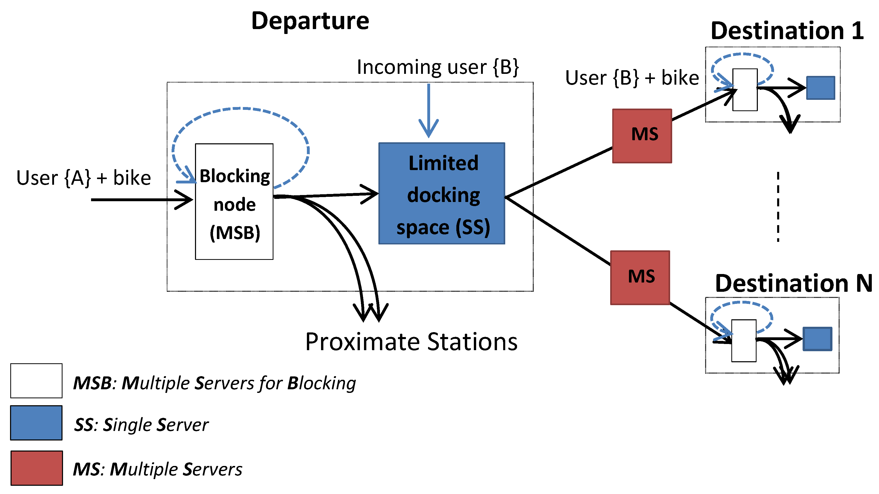
2.1.1. A Bike Station Model

A real bike station equipped with the blocking mechanism is modeled by a couple of queues noted $<MSB,SS>$. The queue $SS$ stands for a Single Server queue and models the real station. The $SS$ queue has a limited capacity that is equal to the docking capacity of the bike station. The $SS$ service time corresponds to the time between the arrival of two users coming to pick up a bike. After the departure of a user {B} with a bike (cf Figure 1), the server of $SS$ becomes available and another bike undergoes a service time waiting for a next user {B}.

Since there are limited capacity queues (i.e., $SS$), a blocking mechanism is assigned to manage the rejected bikes by a full station. We use the Repetitive Service-Random Destination, RS-RD, as the blocking mechanism. In this blocking mechanism, if a job tries to access a full queue j it is immediately returned to the last queue i (departure queue) where the job undergoes a new service time. Afterwards, the job is redirected to a downstream queue, depending on the routing probabilities from the queue i [42].

Accordingly, a multiple server queue $MSB$ is located upstream of every single $SS$. It contains L parallel servers (the fleet size of the BSS). The local process of arrival of bikes to a real bike station is defined as follows:

• Step 1. A bike heading towards the bike station i (user {A} + bike in Figure 1) comes first to its $MS{B}_i$.
• Step 2. A destination (i.e., principal $S{S}_i$ or secondary $S{S}_j,j\ne i$) is chosen according to the routing probabilities in the routing matrix ${\alpha }_{ij},i,j=1,\dots ,M$.

  -

  Step 2-a. If a secondary bike station $<MS{B}_j,S{S}_j>$ (a neighboring station) is chosen, the bike leaves the local process associated with the bike station i.

  -

  Step 2-b. Otherwise, the bike is routed to $S{S}_i$ (the principle destination), then

  *

  Step 2-b1. If, there is at least one free docking space, the bike is dropped. So, the service is successful.

  *

  Step 2-b2. If the $S{S}_i$ is full, the blocking mechanism RS-RD is applied. The bike loops back to $MS{B}_i$ (the dashed arrow in Figure 1). The process returns to the beginning (Go To Step 1).

A short service time in $MSB$ is recommended for two reasons. First, this duration should be short enough to not alter the trip duration between the departure and the destination stations. Second, when a bike is blocked several times in $MSB$, the sum of all iteratively applied service times represents the waiting time of the user before finding a free dock. The outgoing routing probabilities from $MSB$ should be set properly. This means that the routing to the principle $S{S}_i$ must have the highest probability (0.9 for example). The remaining probability is allocated to the close secondary $S{S}_j,j\ne i$ stations.

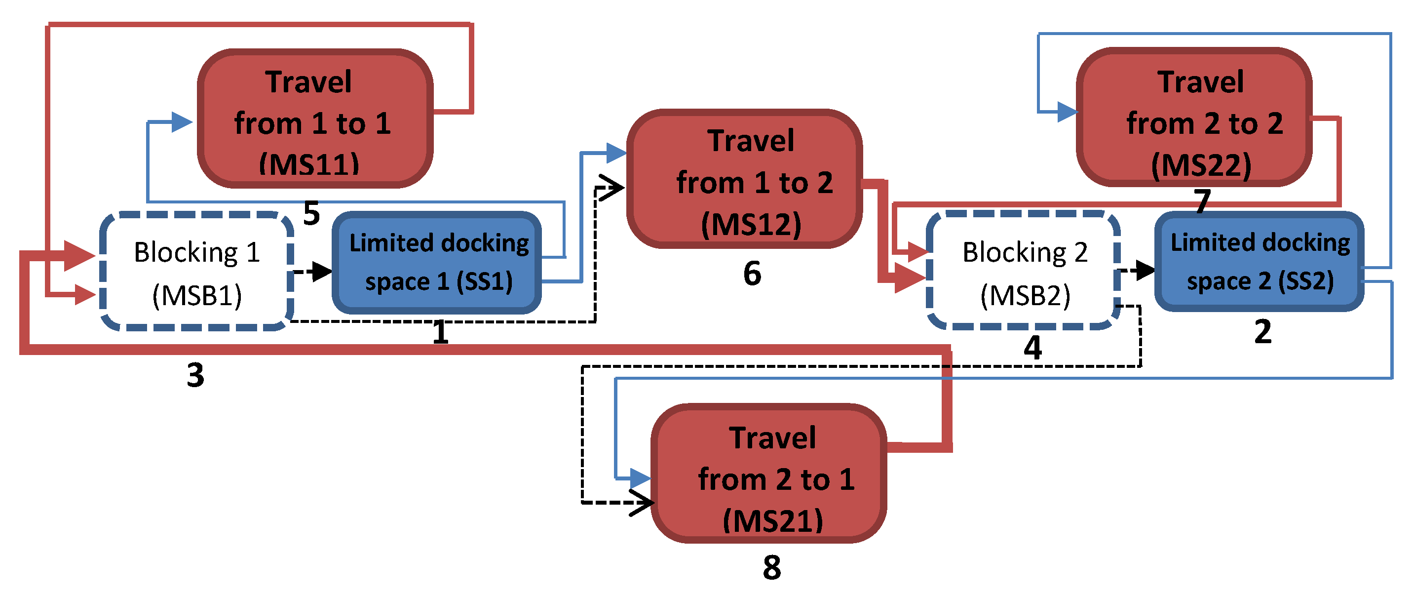
2.1.2. The Model of Trip between Two Stations

The trip between two bike stations is modeled by a Multiple Server (noted $MS$) containing L parallel servers (L is the fleet size). With this configuration, all the BSS bikes could be contained in this queue. The service time of the queue equals the travel time. Figure 1 shows how these queues are connected together.

2.1.3. The Explicit Model of Two Bike Stations

Figure 2 shows the explicit model of two interconnected bike stations 1 and 2. This figure expands the model of George and Xia [31] by introducing the blocking mechanism.

Nodes 1 and 2 in blue represent the two real bike stations ($SS$ nodes). Each $SS$ node is fed by the bikes coming from its virtual blocking node represented by the dotted lines stations ($MSB$ queues). The red queues model the four possibilities of travelling ($MS$ stations) between the two stations.

Hereafter, the routing matrix of the two station system (captured in Figure 2) is defined, considering the indexes in

Table 2. Indexes of the queues in the routing matrix.

Index	1	2	3	4	5	6	7	8
Queue	SS1	SS2	MSB1	MSB2	MS11	MS12	MS22	MS21

.

${\alpha }_{15},{\alpha }_{16},{\alpha }_{27}$ and ${\alpha }_{28}$ capture the probabilities of travelling from a station to another or the probabilities of round trips. The routing probabilities equal 1 when the departure queue corresponds to a travel ($MS$ type). ${\alpha }_{31},{\alpha }_{36},{\alpha }_{42}$ and ${\alpha }_{48}$ are the probabilities defined in the downstream of the blocking nodes ($MSB$ type).

Solving the closed queuing network model means finding out the equilibrium (i.e., steady state) marginal state probabilities (mainly the marginal state probabilities of $SS$ queues) and to deduce the required performance indicators describing the whole system. In the next section, we present the suitable resolution approach for this model. This approach is developed by Kouvatsos and Xenios [40].

3. Resolution of the Closed Network under RS-RD Blocking Using Entropy Maximization Method

3.1. State Space

The BSS is modeled by a closed network under RS-RD blocking mechanism. This network consists of M (First Come First Served) queues with general inter-arrival time and service-time distributions. These queues can either be with a limited capacity (i.e., N) single server (G/G/1/N) or multiple servers with an infinite capacity (G/G/L) where L represents the number of servers. For a given fleet size L, the state space of the network is represented by:

$$\begin{array}{c}\hfill S=\left\{(n_1,\dots ,n_M):\sum _{i=1}^M{n}_i=L,0\le n_i\le N_{vi},i=1,\dots ,M\right\}\end{array}$$

(1)

where $N_{vi}=min(N_i,L)$ is the capacity of the queue i of the network and $N_i$ the capacity of the single server queue i. The state vector $(n_1,n_2,\dots ,n_M)$ is noted from now on $\mathbf{n}$, and the equilibrium probability of the network to be in the state $\mathbf{n}$ is noted $p\left(\mathbf{n}\right)$. Let also $p_i\left(n_i\right)$ be the equilibrium marginal state probability of a queue i containing $n_i$ jobs. By solving this network we seek to calculate the probability of each state $p\left(\mathbf{n}\right)$ that allows to compute the performance indicators associated with the queues. Referring to [40,43], an approximate product form for this network is computed using the Entropy Maximization through an iterative approach. The product-form simplifies the resolution as the queues are considered separately and solved in isolation [44].

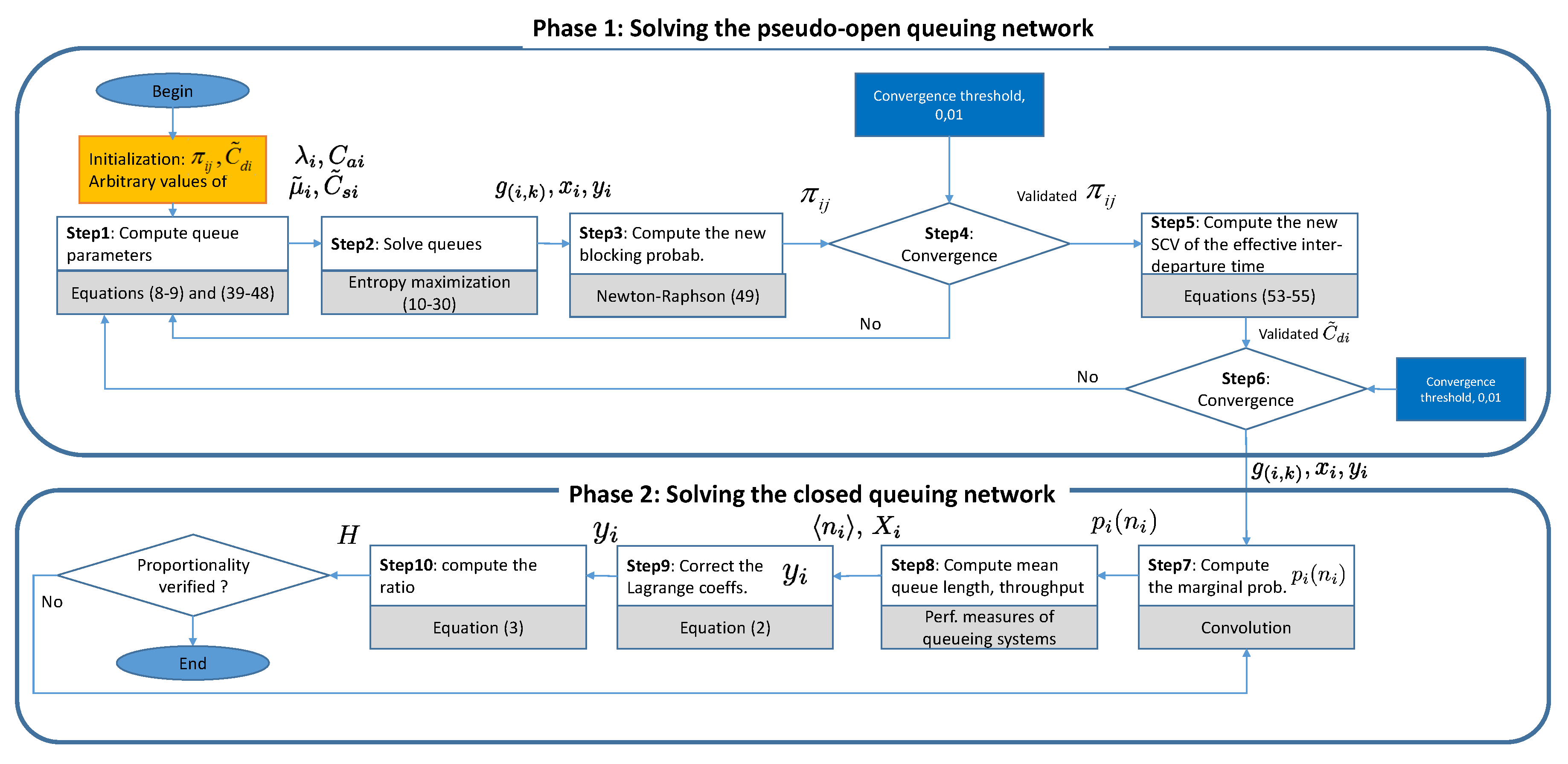
3.2. Procedure for Solving the Closed Network of the BSS Model

The resolution technique [40,43] works in an iterative manner. The analytical formulations and details are shortly provided in the Appendix B. The interested readers are warmly advised to refer to the original papers of Kouvatsos and Xenios. Hereafter, we give a simplified overview of the procedure, depicted in Figure 3.

The closed network is solved in two phases. In a first Phase, the pseudo-open network corresponding to the original closed network is solved. A pseudo-open network is a closed network represented as an open network with no external arrivals and no external departures [42]. Then, during the second Phase the states probability distribution $p\left(\mathbf{n}\right)$ of the original closed network is calculated.

Phase 1-Solving the Pseudo-Open Queuing Network

In an iterative manner, we look for the blocking probabilities ${\pi }_{ij}$ and the scv (squared coefficient of variation) of the effective inter-departure time ${\tilde{C}}_{di}$ of stations. The iterations loop required for ${\tilde{C}}_{di}$ [i.e., Steps 1–6] contains the iterations loop for ${\pi }_{ij}$ [i.e., Steps 1–4] after initialization.

Initialization—The iterations start by some initial arbitrary values of ${\pi }_{ij}$ and ${\tilde{C}}_{di}$.

Step 1—For every queue, the inter-arrival rate and its scv {${\lambda }_i,C_{ai}$} and the effective service time and its dispersion {${\tilde{\mu }}_i,{\tilde{C}}_{si}$} are computed.

Step 2—The queues $i,i=1,\dots ,M$ are individually solved:

• $SS$ queues as censored queues (i.e., those queues $SS$ where the arriving customers are turned away when the buffer is full), (GE(${\lambda }_i$,$C_{ai}$)/GE(${\tilde{\mu }}_i$,${\tilde{C}}_{si}$)/1/0;$N_i$), and
• $MSB$ and $MS$ queues as stable queues (i.e., those queues without capacity limitations) (GE(${\lambda }_i$,$C_{ai}$)/GE(${\tilde{\mu }}_i$,${\tilde{C}}_{si}$)/L).

The resolution technique is based on finding out the Lagrange multipliers maximizing the Entropy function (A3) subject to normalization (A4) and marginal constraints (A5)–(A7). These Lagrange coefficients are $g_{(i,k)}$, $x_i$ and $y_i$ for $i=1,\dots ,M$ and $k=1,\dots ,c_i$.

Step 3—The new values of the blocking probabilities ${\pi }_{ij}$ are calculated from the newly obtained values of $p_i\left(n_i\right)$ and ${\tilde{C}}_{si}$ in Step 2. The resolution looks for finding out the roots of (A42) in the Appendix B by using Newton-Raphson method.

Step 4—The evolution of the blocking probabilities ${\pi }_{ij}$ is then compared with a threshold value (let say 0.01) to conclude the convergence, otherwise return to Step 1.

Step 5—The new values of {${\tilde{C}}_{di}$} (A46) are then computed using the ${\pi }_{ij}$ after the convergence of Steps 1 to 4.

Step 6—The evolution of the effective inter-departure time {${\tilde{C}}_{di}$} is then compared with another threshold defined by the users to conclude the convergence. According to Kouvatsos [43] the convergence is always guaranteed.

Phase 2—Solving the Closed Queuing Network

The resolution of the pseudo-open queuing network gives an estimation of the Lagrange coefficients for the closed queuing network. These parameters are used to find out the state probability p(n) which maximizes the entropy (A26) of the original closed network. This is performed in the rest of the approach.

Step 7—The marginal probabilities $p_i\left(n_i\right)$, $i\in 0,\dots ,M$, for the original CQN are computed using a convolution method.

Step 8—At this step, it becomes possible to calculate the mean queue length $〈n_i〉$ and the throughput $X_i$ for $i=0,\dots ,M$.

Step 9—The Lagrange Coefficients obtained from the resolution of the pseudo-open network (noted by ${\tilde{y}}_i$), obtained in Step-2, are then revised by using the following formula, knowing now $〈n_i〉$ and $X_i$. These coefficients $y_i$ correspond to the constraint of the state probabilities of the full $SS$ queues (A7).

$$y_i={\tilde{y}}_i{\tilde{\lambda }}_{i}L{\left[X_i\sum _{j=1}^M\frac{{\lambda }_j〈n_j〉}{X_j}\right]}^{-1}$$

(2)

Step 10—Return to step 7 and adjust the throughput to satisfy the flow balance equations (A1) till obtaining the same ratio of the rate of the effective inter-arrival-time to the throughput (3) for all the queues.

$$H=\frac{{\tilde{\lambda }}_i}{X_i}i=1,\dots ,M$$

(3)

3.3. Performance Indicators of the BSS

This resolution technique allows to compute the following performance indicators for a real station i.

• Availability of bikes is the probability of finding at least one bike at $S{S}_i$.

  $$A{b}_i=1-p_i(n_i=0)$$

  (4)
• Availability of docks is the probability of finding at least one free dock at $S{S}_i$.

  $$A{d}_i=1-p_i(n_i=N_i)$$

  (5)
• Aggregate performance of a station is the weighted combination of both availabilities.

  $$Ap{s}_i=a_{i}A{b}_i+b_{i}A{d}_i$$

  (6)
• Overall performance of the network computes the normalized overall performance of all stations of the network.

  $$Gpn=\frac{1}{N_T}\sum _{i=1}^{N_T}{a}_{i}A{b}_i+b_{i}A{d}_i$$

  (7)

  with $a_i+b_i=1,i=1,\dots ,N_T$ where $N_T$ represents the number of bike stations.

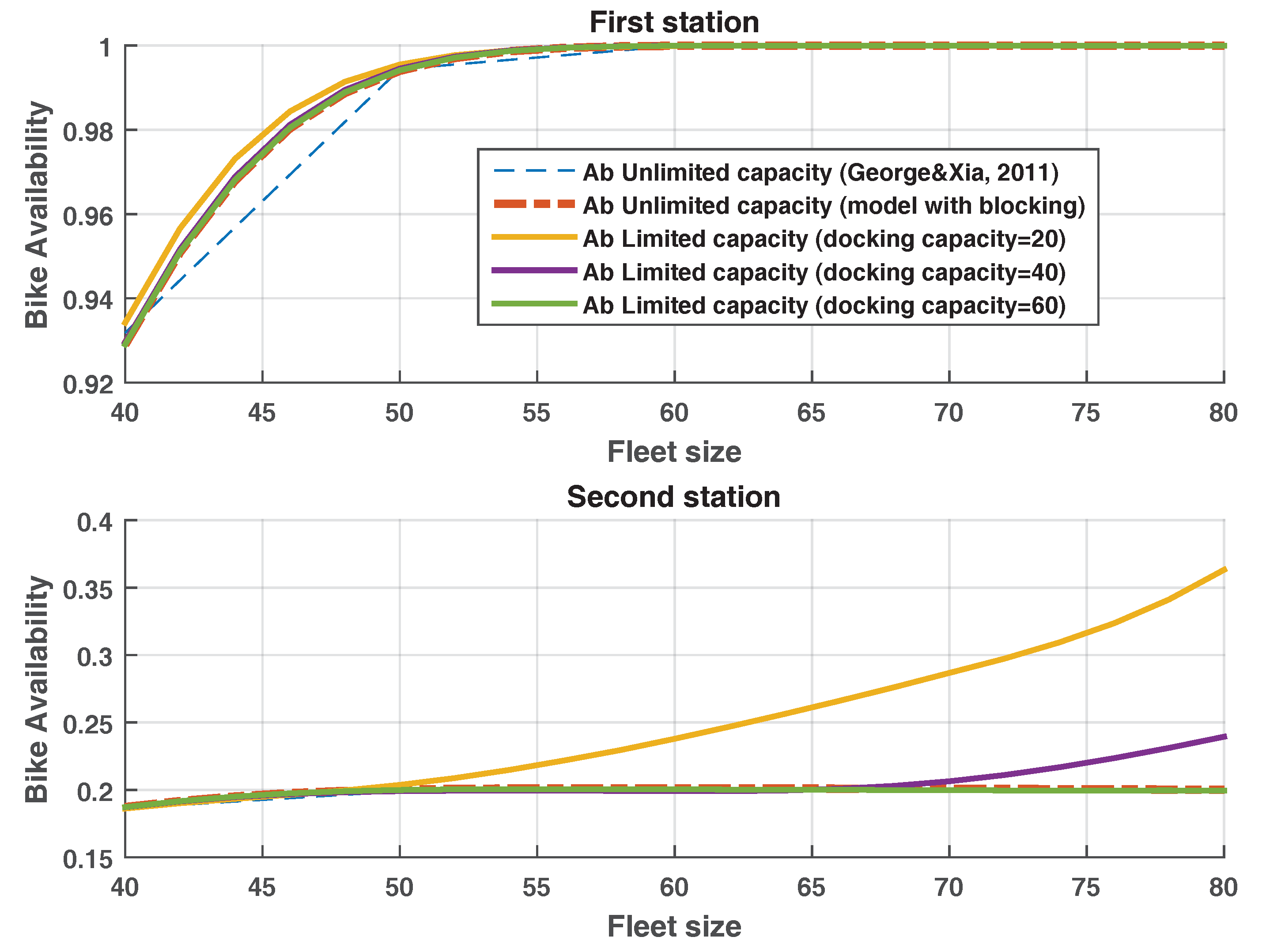
3.4. Comparison and Validity Testing

To validate the suggested model in this paper, the published model exposed by the authors in [31] is considered as a reference. The parameters of our model (namely, the bike stations capacity and the routing probabilities) are modified to represent the same unlimited capacity situation as for the one of reference model. We then execute the new model and compare the results with the reference model results. The conformance of the new model results and those ones obtained by the reference model is studied. As it can be seen hereafter, the results are almost the same. Finally, we introduce three limited capacity scenarios in our model to highlight the awaited reduction of the bike availability rates.

The studied case by [31] (p. 7) is defined by a network of two stations with unlimited capacity. The routing probabilities between these stations are gathered in the following matrix R.

$$R=\left[\begin{array}{cc}0.9& 0.1\\ 0.5& 0.5\end{array}\right].$$

The arrival rate of users to the stations is 15 users/hour and the mean trip duration is 2 h. We build and parametrize our model to reproduce the conditions of George and Xia’s model. Figure 4 shows the perfect superposition of these results and those of the original work of George and Xia; the reference model. This conformance shows the reliability of the suggested model with the blocking mechanism.

In order to show the impact of a limited capacity, and therefore the necessity of its consideration, three scenarios are solved and the bike availabilities are computed, see Figure 4. For each scenario, the two stations have the same capacity (20 docks, 40 docks and 60 docks).

For these three scenarios, the service duration of the $MSB$ queues is 1/120 h and the routing probability from one $MSB$ queue to $SS$ queue (the station) is 0.999 to force bikes to enter the bike station. The remaining probability allows to route the rejected bikes to the other station.

Relying on the evolution of the bike availability due to the limited capacity, two main observations can be made:

-

Introducing the limited capacity of the stations has a direct influence on the bike availability. Due to the routing probabilities in R, the first station is saturated. The bikes leaving the first station are routed mainly to the same station (i.e., 0.9) as shown in R. Moreover, this station receives bikes from the second station too (i.e., 0.5). This explains the high bike availability of the station 1 in all the three scenarios, which approximately, matches with the unlimited capacity scenario.

-

The difference between the scenarios, regarding the bike availability, is much more important for the second station than the first one. Due to the unbalanced routing probabilities, the second station receives fewer bikes than the first station. In the limited capacity scenarios, the more the fleet size is increased the more the second station is saturated compared to the unlimited capacity model. In fact, because of the limited capacity, the first saturated station would reject bikes as the fleet becomes bigger. Therefore, the blocking mechanism would redirect the bikes to the second station. As the docking capacity becomes bigger, the bike availability of the second station increases and tends to the value of the bike availability (Ab) in the unlimited capacity model.

It can be concluded that the model supporting the limited capacity stations with the blocking mechanism extends the unlimited capacity station model defined in [31] providing a more realistic bike availability; the original model of George and Xia gives an over-estimated bike availability.

4. Numerical Results for a Subset of 20 Stations of Paris Velib

4.1. Data Analysis and Hypothesis

The Velib system consists of almost 1700 stations and 23,000 bikes [45]. The resolution algorithm is time consuming for the whole network. The computation complexity of the algorithm is $O\left(k_1{(\mathsf{\Omega }+1)}^3\right)$ for Phase 1 and of $O\left(k_2{M}^2{L}^2\right)$ for Phase 2 [40], where $k_1$ is the number of iterations for steps 1–6, $k_2$ is the number of execution of the loop in steps 7–10 and $\mathsf{\Omega }$ is the cardinality of $\{{\pi }_{ij}:i,j=1,\dots ,M;i\ne j\}$ (i.e., $\mathsf{\Omega }=N_T$, $N_T$ is the number of stations of the BSS). Accordingly, it is decided to focus on a small geographic zone with a limited number of stations (20 stations). We considered 3 stations in “Ile de la Cite” at the very center of Paris. The other 17 stations are the most visited destination stations from these three stations. These stations are located in touristic zones and have a stable usage rate [46]. The data is collected for a period of 30 days, between the 5 of September and 15 of October 2016, excluding the weekends. This period is characterized by the homogeneity of the weather conditions. Data is collected from the Open database of the operator of Velib and treated to derive the parameters such as the rate, scv of the service time of the queues and the routing matrix.

We focus on the time points where bikes are picked up in one of these 20 stations and brought from other stations to these stations. The inter-arrival rate of users to stations is obtained from the inter-departure rate of bikes; the inter-arrival rate of users to a station equals the inter-departure of bikes when there is at least one bike at the station. We process the data by considering only the states where non-empty condition is met. We estimate the number of the users arriving to pick up the bikes at each station by an hour time slot for every day; in fact, we consider the duration of the inter-departure of bikes and we exclude the data collected just after an empty state of a station. For every time slot, the mean arrival rate and its dispersion are computed over all the days of the studied period. The duration of time that we focus on in this study is from 8 a.m. to 10 a.m. corresponding to the rush hours. This choice is mainly due to the similarity between the 8–9 a.m. and 9–10 a.m. time slot. Thus, the proposed model evaluates the steady-state performance of the system corresponding to the mean performance in this time-window.

The trip durations, their rates and the squared coefficient of variations are extracted from the raw data. This gives the necessary parameters of the $MS$ queues of the model. Regarding the routing probabilities between the stations (i.e., from the bike stations ($SS$) to the paths ($MS$)), the raw data for the whole year 2016 is cleaned by eliminating the weekends and the special events for the purpose of achieving more reliability. The routing probability from a departing station to a destination station equals to the ratio between the number of trips to this destination and the sum of all the trips departing from the origin station. By this way, the routing probabilities between the stations in the studied zone and from-and-to the exterior stations are also computed. After selecting the (sub)network, the aforementioned closed queuing model resolution technique (Section 3) is used even if the (sub)network cannot be considered as a real closed network. However, selecting the most visited stations from the three central stations greatly limits the side effects of the connection between the considered zones (the 20 stations) and the rest of the network. This issue is discussed in the conclusions and perspectives section of the paper.

Since there is no data information regarding the willingness of users to look for neighboring stations or to wait for an empty dock to lock a bike, the routing probabilities from an $MSB$ queue to a principal $SS$ queue are chosen arbitrary (i.e., between 0.8 and 0.9) and the remaining probabilities are assigned to the neighboring stations [3].

4.2. Experiments and Results

The resolution method of the model of 20 stations was programmed and implemented in Matlab. We study the effects of the fleet size, docking capacity, inter-arrival rate of users picking up bikes and flow of incoming bikes to a station on the system performance. The resolution algorithm, set by the collected input data, is made open access (goo.gl/AsynMX).

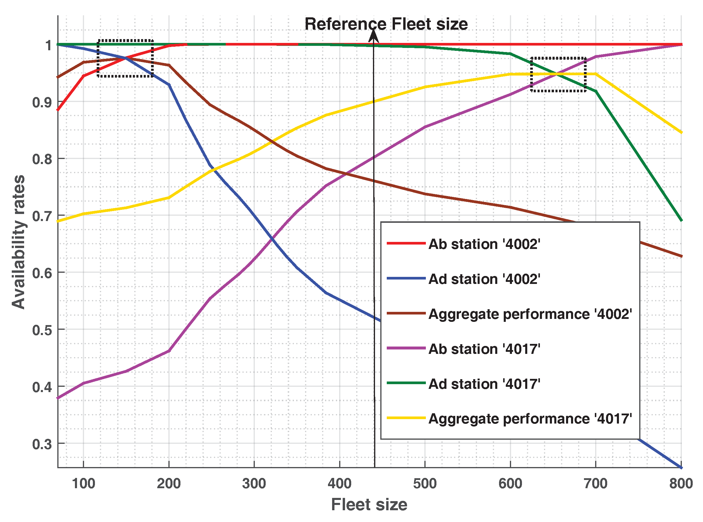
• Fleet-sizing: impact on dock and bike availability. The fleet sizing is accomplished through the change of the parameter L in the model. The stations are affected differently. Only the availability rates of two typical stations: 4002 and 4017 are presented in Figure 5.

It can be noticed that the bike availability ($Ab$, see (4)) of stations increases when the fleet size increases and tends towards 100%.

As a result of unlimited capacity, George and Xia [31] conclude that the availability does never reach 100% for the non-saturated stations. However, in our case, for the limited capacity BSS model, it is shown that even stations that do not attract bikes can be saturated for high fleet sizes. In fact, whenever the fleet size is big, the rejected bikes from the full stations are redirected to fill the empty stations.

On the contrary, the dock availability ($Ad$, see (5)) decreases from 100% as the fleet size increases. This opposite evolution of the two curves creates a crossing point. The crossing point appears in all the stations and reflects an interesting zone of performance, which is the best performance area: both availability indicators are higher than 0,95. This area is represented by a dashed rectangle in Figure 5. This behavior is observed in all bike stations omitted from this paper.

Figure 5 shows the aggregate performance of a station ($A_{ps}$, see (6)). Since it is interesting to consider bikes and docks availability, it is decided to give the same importance to both indicators. In a real situation, the system operator could attribute different coefficients according to the dynamic situation of stations (e.g., a bike station close to a transport hub).

Stations reach the performance area for a different fleet size; the optimal fleet size for the station 4002 is 150 while for the station 4017 is 650 bikes. Therefore, when we involve all the stations, it is necessary to compute the fleet size taking account of all the stations. Figure 6 shows the evolution of the overall network performance indicator ($G_{pn}$, see (7)) as a function of the fleet size where the two availabilities have equal importance, i.e., $(a_i=b_i=0.5,i=1,\dots ,N_T,N_T=20)$. The system operator can be interested in evaluating the overall availability to make decisions for the whole network.

Interestingly, the overall performance curve shows a flat performance area between 380 and 520 bikes. This means that the whole (sub)network has a very robust behavior regarding the fleet size; the overall performance is about 88% for a fleet size varying between these two extreme values. The analysis can be completed by considering a “reference fleet size”. This reference fleet size is 440 bikes corresponding to the middle of this large span of fleet size. In [47], the authors reveal that in most of the bike sharing systems (Montreal, London, etc.), the operators use an experimental ratio of docking capacity to a fleet size of 2–2.5. If we apply this rule in our case we will find out that the fleet size should be between 248 and 310 bikes, since the total capacity of the 20 stations is 621 docks. Accordingly, by following this rules, operators are leveraging the docking availability at the expense of the availability of bikes. In our case, we have given the same importance to both availability indicators.

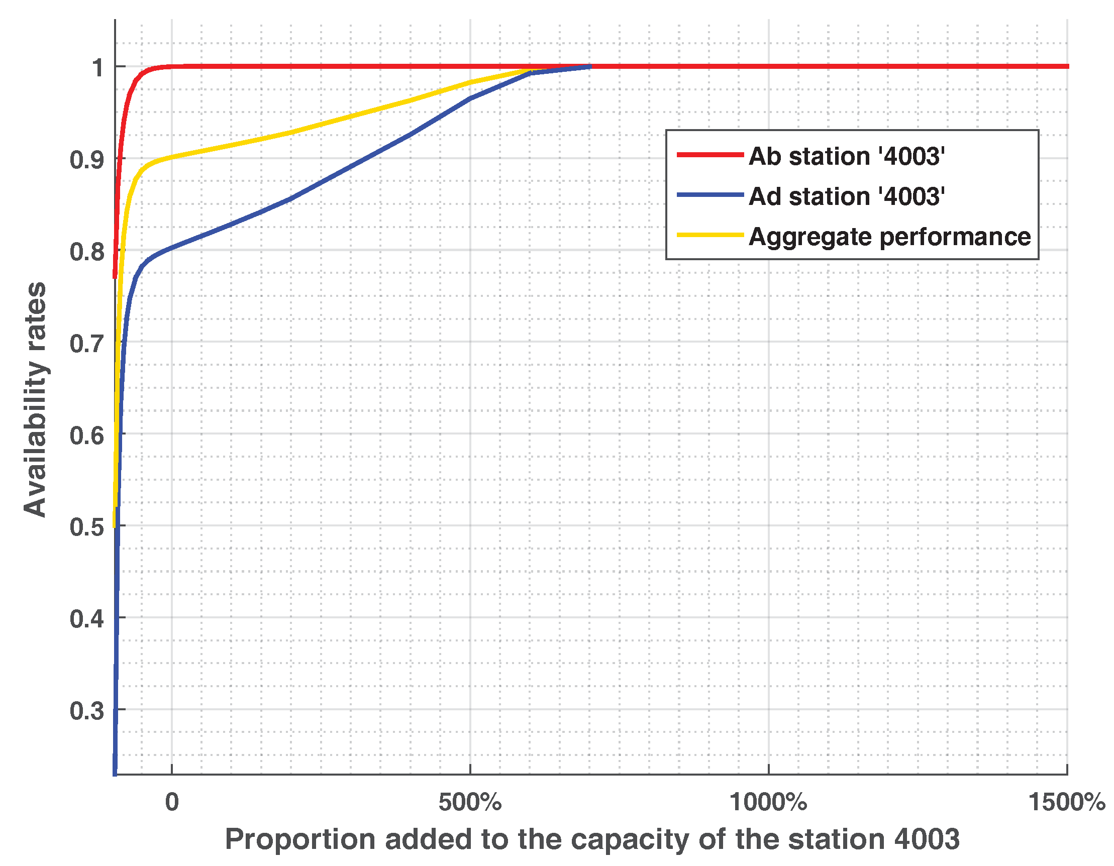
• Docking capacity. To visualize the effect of the docking capacity, the number of docks of the station 4003 is modified by adding or removing a proportion of its actual capacity (20 docks) as shown in Figure 7.

When the capacity increases, the availability of bikes remains constant. The chance of finding a free dock increases. So, to overcome the shortage of docks, the capacity of the station should be enlarged. Nevertheless, the 100% aggregate performance may be reached by 140 more docks (700% of capacity increase). It is not realistic to target this ultimate level of performance for evident reasons (cost, place, etc.).

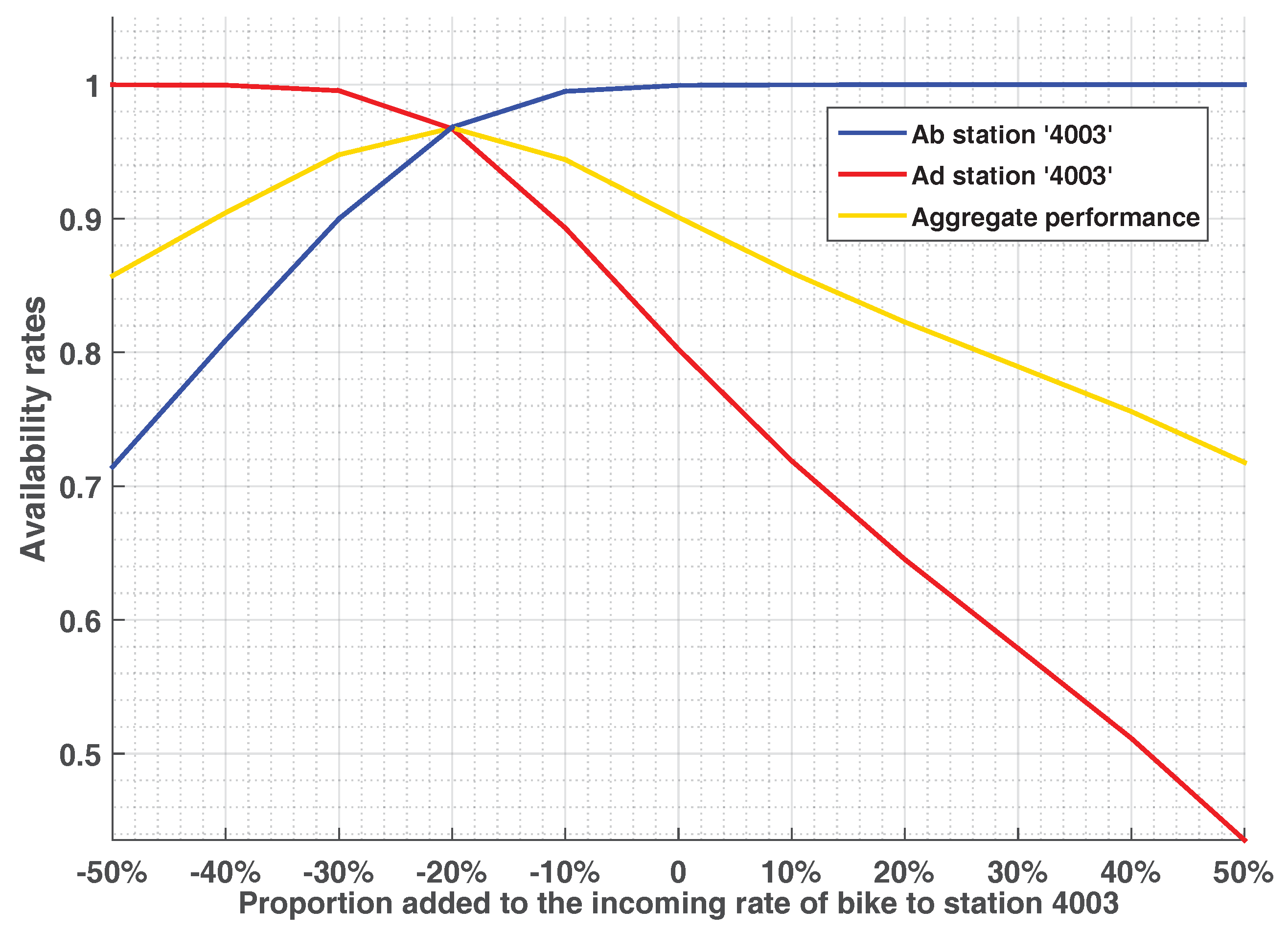
• Incoming flow variation. It is possible to modify the incoming flow of bikes to stations by an economic incentive for instance [9]. In this experiment, we would like to find out how the performance of the station 4003 evolves as a function of the incoming flow. This effect is represented in Figure 8.

For the initial incoming flow rate, the availability of bikes is 100% but the chance of finding a free dock is lower, i.e., 80%. We would like to know whether any change in the incoming flow could increase the dock availability without a serious deterioration of the bikes availability. By focusing on the aggregate performance of the station (same importance of bike and dock availabilities) in Figure 8, it can be seen that the maximum rate is achieved at the incoming flow of −20% and this ensures very good bike and dock availabilities (about 96%). This result is coherent because this station has a tendency to be full. So, it is reasonable to reduce its incoming flow of bikes (here by 20%) to make it “less” full while allowing a good bike availability.

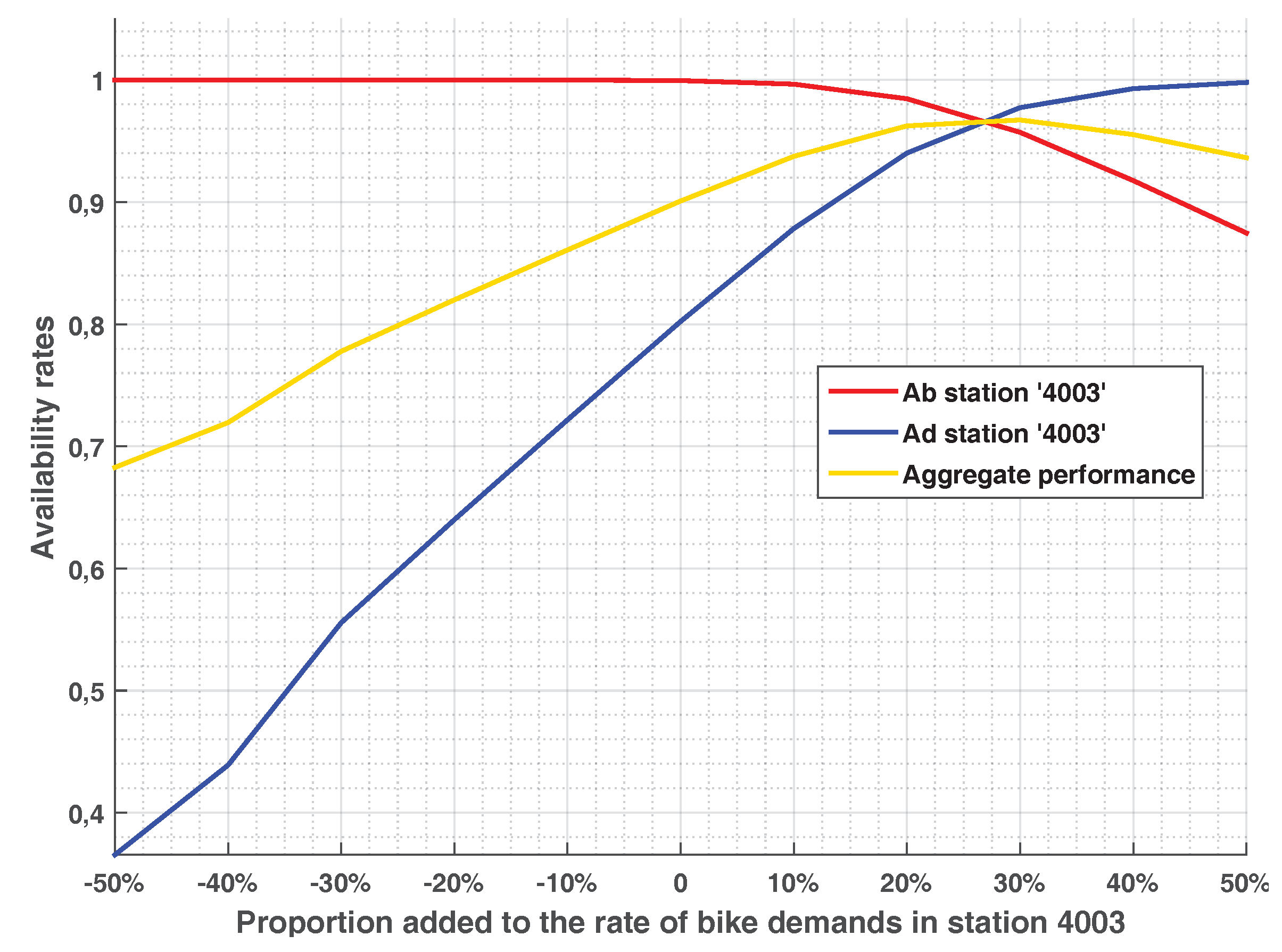
• Demands for bikes variation. It is also possible to increase the demand of bikes (to drain the bikes from saturated or almost saturated stations) by starting some economic incentives. We would like to know whether a BSS operator may launch such incentives to improve the performance of stations.

Figure 9 shows these experiments where the bike and dock availabilities and the aggregate performance of the station are computed as a function of the variation of the arrival rate of users to the station 4003. For the initial value of the arrival rate, the dock and bike availabilities are 80% and close to 100%, respectively. The highest aggregate performance is obtained following an increase of 27% of the arrival rate where both availabilities are about 97%. This result is consistent because the station 4003 tends to be full. Accordingly, increasing the demand rate increases the dock availability (Ad) but slightly decreases the bike availability (Ab).

4.3. Discussion of the Obtained Results

By monitoring or controlling the BSS, the system manager seeks to reach the best performances for the stations and the entire system. This would be achieved for the whole day and particularly for the peak hours. In these experiments, we have focused on the performance of a (sub)network during the morning rush hours, from 8am to 10am.

Our experiments show that modifying the used parameters will modify the bike and dock availabilities which evolve in opposite direction. So, trade-offs between both availabilities should be found. In this respect, the aggregate performance of a station seems to be a good indicator on which the operator can rely. It is simple and can reflect the local target for every studied station taking into account of the station’s specificities by weighting appropriately both availabilities.

Control-oriented decisions: Robustness of the overall performance of the network regarding the fleet size. Practically, the BSS operator does control actions by adding the number of bikes and/or docks to increase the users satisfaction. While studying the fleet size, it is noticed that every station has a different optimal fleet size regarding its aggregated performance (6). This clearly suggests that finding out the optimal fleet size for the whole (sub)network should go through trade-offs among the stations on the ground that some stations could be more critical than others. In our case study, the stations are located at the touristic sites and are considered as critical. In other cases, it depends on the users satisfaction to be achieved regarding the station geographical position (i.e., stations close to the working area or transport hubs, etc.). In a top-down analysis, the operator may first find out the “best” fleet size which maximizes the overall performance (7) of the whole (sub)network. We have noticed that this overall performance is not very sensitive to the fleet size for a large size span (between 380 and 500 bikes). The overall performance is quite robust regarding this parameter. It is therefore possible to adjust the fleet size by considering the size that increases the performances of the critical stations in a second step.

Control-oriented decisions: The overall performance not highly sensitive to capacity. As the second control action, we evaluate the capacity change of a station. It was observed that the increase of the capacity of a station which tends to be saturated, improves the availability of docks locally in the station. The aggregate performance (6) evolves slowly by a drastic increase of the station capacity (700% for station 4003). However, the overall performance of the network (7) declines due to the deterioration of the availability of bikes in the other stations. In other words, the stations with an increased capacity absorb these rejected bikes which are not distributed to the other stations. Other experiences of capacity change were performed on the station (4017) which tends to be empty (not presented in this paper). When reducing the station capacity by small amounts, there is no major impact. But when reducing greatly the number of docks, the bike and dock availabilities decrease to a great extent. Therefore, suppressing the remaining docks also suppresses also the few remaining bikes. These bikes are then redirected to the other stations but do not affect the other stations performance due to their negligible number. We conclude then that the capacity change could not be effective to enhance the overall performance.

Effect of monitoring decisions: The overall performance robust to the departure and arrival of bikes to stations. In terms of monitoring operations, there are instantaneous corrective measures that can be considered by the operator to gain better performances. Acting locally on a station by changing its attractiveness seems to be very interesting. The curves in Figure 8 and Figure 9 show that locally, modifications of the arrival and departure rates of bikes to stations directly impact their aggregate performance (6). However, the overall performance (7) remains again relatively robust around the best rates. This is due to the fact that this change does not have any significant influence on the other stations. This shows that the monitoring operation can be performed on a specific station. The monitoring actions are performed now by redistribution of bikes by truck, but our experiments show that the effect of economic incentives are more effective. Decreasing the service price during the rush hours can lower the occurance of extreme cases: empty or full states of the stations.

5. Conclusions and Perspectives

The conclusions of this research can be listed as follows:

Modeling and resolution. In this work, a closed queuing network supporting a blocking mechanism was used to model and assess the performance of a BSS. Accordingly, a resolution approach based on the Entropy maximization was applied. The originality of this work resides in its ability to model in a more realistic way the dynamics of stations and the network. We started from the initial model developed by George and Xia [31]. In their model, the capacity of stations was unlimited. We limited it to make it fit real world constraints, then calculated the dock availability. It was observed that the limited capacity of a station directly affects the bike availability and the unlimited capacities lead to error-prone decisions.

Methodological issues. The performance of a BSS is determined by the bikes and docks availability. The aggregate performance of a station is a compound of those two indicators (bike and dock availability). The aggregate performance reflects the specificities of each station. These performance indicators are used for monitoring, controlling and (re-)designing decisions. If we focus on the first two decisions, we conclude that monitoring decisions aim at improving the system performance on a short-term basis by proposing incentives to the users. In our case, this aspect was indirectly studied by adjusting the bikes arrival and departure (demand). Control decisions are more expensive and tend to guarantee more sustainable performances. They deal with the fleet and capacity sizing.

Experiments and discussions. As the resolution is complex and time-consuming, it was decided to model a (sub)network of the Paris BSS composed of 20 stations. Following a strict experimentation protocol, real data was gathered, pre-treated, and used for experiments. Two sets of experiments on monitoring and control decision were conducted. The results allowed to draw the following conclusions:

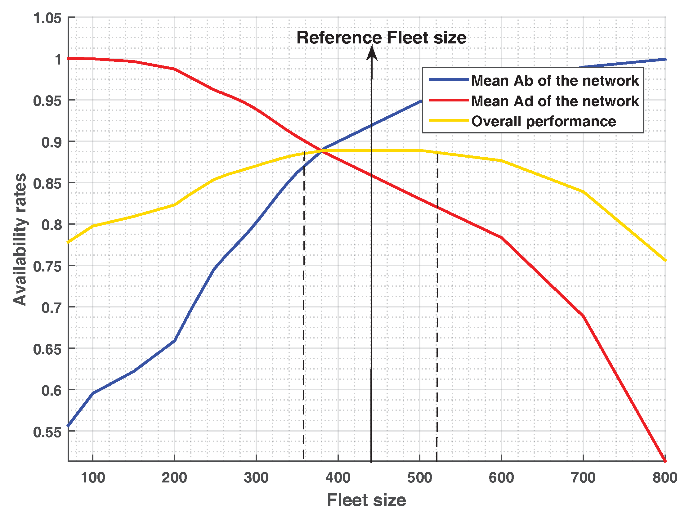
• Control decisions: fleet-sizing. Fleet-sizing has a positive influence on the bike availability but degrades the dock availability if the fleet is too large. Locally, every station has an optimal fleet size that maximizes its aggregate performance. From the point of view of the network, the overall performance is quite robust for a relatively “large” fleet size span.
• Control decisions: capacity-sizing. The overall performance of the network deteriorates if the capacity is changed. The system manager should not consider this option to improve the performances.
• Changes in the arrival and departure flows of bikes. Locally, the modification of the bikes arrival to and departure from a station is very effective with a concrete impact on the aggregate performance of the station. The stations can be targeted for improvement without being concerned with impacts on other stations. These changes can be the effects of the monitoring decisions. These monitoring decisions may be cheaper than the techniques that operators are using now (bikes displacements by trucks). However, their effectiveness requires a deeper economical study.

Despite these practical recommendations related to the BSS monitoring and control decisions, there are some shortcomings that should be improved in the future. As the resolution of the model is tedious and time consuming, a (sub)network of the real BSS was chosen for the experiments. Isolating such a (sub)network requires further research to evaluate the side effects of the exchanges between the (sub)network stations and the stations outside the (sub)network. However, there is hopefully no need to take the whole network into account while focusing on a (sub)network. As matter of fact, statistics show that nearly none of the trips recorded in Paris lasted longer than 30 min from a given station [3].

Another alternative that authors actually consider in order to tackle the complexity of the model, is reducing the number of stations in a (sub)network through the introduction of virtual stations.

We note that re-design operations can also be evaluated using this model. Opening a new station or closing an old one may improve the system efficiency. The financial dimension, i.e., cost versus investment, should be taken into consideration in the decision making process.

Finally, control and design operations of a hybrid BSS (i.e., containing mechanical and electrical bikes) can be evaluated using a network of multiclass jobs.

References

1. Shaheen, S.A. Introduction Shared-Use Vehicle Services for Sustainable Transportation: Carsharing, Bikesharing, and Personal Vehicle Sharing across the Globe. Int. J. Sustain. Transp. 2013, 7, 1–4. [Google Scholar] [CrossRef]
2. Laporte, G.; Meunier, F.; Wolfler Calvo, R. Shared mobility systems. 4or 2015, 13, 341–360. [Google Scholar] [CrossRef]
3. Nair, R.; Miller-Hooks, E.; Hampshire, R.C.; Bušić, A. Large-Scale Vehicle Sharing Systems: Analysis of Vélib’. Int. J. Sustain. Transp. 2013, 7, 85–106. [Google Scholar] [CrossRef]
4. Shi, J.G.; Si, H.; Wu, G.; Su, Y.; Lan, J. Critical factors to achieve dockless bike-sharing sustainability in China: A stakeholder-oriented network perspective. Sustainability 2018, 10, 2090. [Google Scholar] [CrossRef]
5. Kadri, A.A.; Kacem, I.; Labadi, K. A branch-and-bound algorithm for solving the static rebalancing problem in bicycle-sharing systems. Comput. Ind. Eng. 2016, 95, 41–52. [Google Scholar] [CrossRef]
6. Ho, S.C.; Szeto, W.Y. GRASP with path relinking for the selective pickup and delivery problem. Expert Syst. Appl. 2016, 51, 14–25. [Google Scholar] [CrossRef]
7. Preisler, T.; Dethlefs, T.; Renz, W. Self-Organizing Redistribution of Bicycles in a Bike-Sharing System based on Decentralized Control. In Proceedings of the Federated Conference on Computer Science and Information Systems, Gdansk, Poland, 11–14 September 2016; Volume 8, pp. 1471–1480. [Google Scholar] [CrossRef]
8. Lin, J.J.; Wang, N.L.; Feng, C.M. Public bike system pricing and usage in Taipei. Int. J. Sustain. Transp. 2017, 11, 633–641. [Google Scholar] [CrossRef]
9. Li, L.; Shan, M. Bidirectional incentive model for bicycle redistribution of a bicycle sharing system during rush hour. Sustainability 2016, 8, 1299. [Google Scholar] [CrossRef]
10. Nair, R.; Miller-Hooks, E. Equilibrium network design of shared-vehicle systems. Eur. J. Oper. Res. 2014, 235, 47–61. [Google Scholar] [CrossRef]
11. Lin, C.C.; Chen, X.R.; Chang, J.W.; Jiang, X.Y.; Lo, S.C. Replenishment Strategies for the YouBike System in Taipei. In Proceedings of the Institute of Industrial Engineers Asian Conference 2013; Lin, Y.K., Tsao, Y.C., Lin, S.W., Eds.; Springer: Berlin, Germany, 2013; pp. 389–396. [Google Scholar]
12. Garcia-Gutierrez, J.; Romero-Torres, J.; Gaytan-Iniestra, J. Dimensioning of a Bike Sharing System (BSS): A Study Case in Nezahualcoyotl, Mexico. Procedia 2014, 162, 253–262. [Google Scholar] [CrossRef]
13. Mizuno, S.; Iwamoto, S.; Seki, M.; Yamaki, N. Proposal for optimal placement platform of bikes using queueing networks. SpringerPlus 2016, 5, 2071. [Google Scholar] [CrossRef] [PubMed]
14. Gast, N.; Massonet, G.; Reijsbergen, D.; Tribastone, M. Probabilistic Forecasts of Bike-Sharing Systems for Journey Planning. In Proceedings of the 24th ACM International on Conference on Information and Knowledge Management (CIKM 2015), Melbourne, Australia, 19–23 October 2015; pp. 703–712. [Google Scholar] [CrossRef] [Green Version]
15. Montoliu, R. Discovering mobility patterns on bicycle-based public transportation system by using probabilistic topic models. Adv. Intell. Soft Comput. 2012, 153, 145–153. [Google Scholar]
16. Bordagaray, M.; Dell’Olio, L.; Fonzone, A.; Ibeas, Á. Capturing the conditions that introduce systematic variation in bike-sharing travel behavior using data mining techniques. Transp. Res. Part C Emerg. Technol. 2016, 71, 231–248. [Google Scholar] [CrossRef]
17. Jiménez, P.; Nogal, M.; Caulfield, B.; Pilla, F. Perceptually important points of mobility patterns to characterise bike sharing systems: The Dublin case. J. Transp. Geogr. 2016, 54, 228–239. [Google Scholar] [CrossRef]
18. Du, M.; Cheng, L. Better understanding the characteristics and influential factors of different travel patterns in free-floating bike sharing: Evidence from Nanjing, China. Sustainability 2018, 10, 1244. [Google Scholar] [CrossRef]
19. Hu, S.R.; Liu, C.T. An optimal location model for a bicycle sharing program with truck dispatching consideration. In Proceedings of the 2014 17th IEEE International Conference on Intelligent Transportation Systems (ITSC 2014), Qingdao, China, 8–11 October 2014; pp. 1775–1780. [Google Scholar] [CrossRef]
20. Li, L.; Shan, M.; Li, Y.; Liang, S. A Dynamic Programming Model for Operation Decision-Making in Bicycle Sharing Systems under a Sustainable Development Perspective. Sustainability 2017, 9, 895. [Google Scholar] [CrossRef]
21. Pal, A.; Zhang, Y. Free-floating bike sharing: solving real-life large-scale static rebalancing problems. Transp. Res. Part C 2017, 80, 92–116. [Google Scholar] [CrossRef]
22. Clemente, M.; Fanti, M.P.; Iacobellis, G.; Ukovich, W. A discrete-event simulation approach for the management of a car sharing service. In Proceedings of the 2013 IEEE International Conference on Systems, Man, and Cybernetics (SMC 2013), Manchester, UK, 13–16 October 2013; pp. 403–408. [Google Scholar] [CrossRef]
23. Clemente, M.; Fanti, M.P.; Mangini, A.M.; Ukovich, W. The Vehicle Relocation Problem in Car Sharing Systems: Modeling and Simulation in a Petri Net Framework. In Proceedings of the International Conference on Applications and Theory of Petri Nets and Concurrency, Milan, Italy, 24–28 June 2013; Springer: Berlin/Heidelberg, Germany, 2013; pp. 250–269. [Google Scholar]
24. Fanti, M.; Mangini, A.; Pedroncelli, G.; Ukovich, W. A Petri Net model for fleet sizing of Electric Car Sharing Systems. In Proceedings of the 2016 13th International Workshop on Discrete Event Systems (WODES), Xi’an, China, 30 May–1 June 2016; pp. 51–56. [Google Scholar] [CrossRef]
25. Labadi, K.; Benarbia, T.; Barbot, J.P.; Hamaci, S.; Omari, A. Stochastic Petri Net Modeling, Simulation and Analysis of Public Bicycle Sharing Systems. IEEE Trans. Autom. Sci. Eng. 2015, 12, 1380–1395. [Google Scholar] [CrossRef]
26. Febbraro, A.; Sacco, N.; Saeednia, M. One-Way Carsharing Solving the Relocation Problem. Transp. Res. Rec. 2012, 2319, 113–120. [Google Scholar] [CrossRef]
27. Kaspi, M.; Raviv, T.; Tzur, M. Parking reservation policies in one-way vehicle sharing systems. Transp. Res. Part B 2014, 62, 35–50. [Google Scholar] [CrossRef]
28. Barth, M.; Todd, M. Simulation model performance analysis of a multiple station shared vehicle system. Transp. Res. Part C 1999, 7, 237–259. [Google Scholar] [CrossRef]
29. Fishman, G.S. Discrete-Event Simulation Modeling, Programming, and Analysis, 1st ed.; Springer: New York, NY, USA, 2001. [Google Scholar]
30. Baskett, F.; Chandy, K.; Muntz, R.; Palacios-Gomez, F. Open, closed, and mixed networks of queues with different classes of customers. J. Assoc. Comput. Mach. 1975, 22, 248–260. [Google Scholar] [CrossRef]
31. George, D.K.; Xia, C.H. Fleet-sizing and service availability for a vehicle rental system via closed queueing networks. Eur. J. Oper. Res. 2011, 211, 198–207. [Google Scholar] [CrossRef]
32. Fanti, M.P.; Mangini, A.M.; Pedroncelli, G.; Ukovich, W. Fleet sizing for electric car sharing system via closed queueing networks. In Proceedings of the 2014 IEEE International Conference on Systems, Man and Cybernetics (SMC), San Diego, CA, USA, 5–8 October 2014; pp. 1324–1329. [Google Scholar] [CrossRef]
33. Fricker, C.; Gast, N. Incentives and redistribution in homogeneous bike-sharing systems with stations of finite capacity. EURO J. Transp. Logist. 2014, 5, 261–291. [Google Scholar] [CrossRef] [Green Version]
34. ter Beek, M.H.; Gnesi, S.; Latella, D.; Massink, M. Towards Automatic Decision Support for Bike-Sharing System Design. In Proceedings of the International Conference on Software Engineering and Formal Methods, York, UK, 7–8 September 2015; Bianculli, D., Calinescu, R., Rumpe, B., Eds.; Springer: Berlin/Heidelberg, Germany, 2015; Volume 9509, pp. 266–280. [Google Scholar] [CrossRef]
35. Fricker, C.; Bourdais, C. A Stochastic Model for Car-Sharing Systems. arXiv, 2015; arXiv:1504.03844. [Google Scholar]
36. Fricker, C.; Gast, N.; Mohamed, H. Mean field analysis for inhomogeneous bike sharing systems. In Proceedings of the DMTCS 2012, Montreal, QC, Canada, 18–22 June 2012; pp. 365–376. [Google Scholar]
37. Fricker, C.; Servel, N. Two-choice regulation in heterogeneous closed networks. Queueing Syst. 2016, 82, 173–197. [Google Scholar] [CrossRef]
38. Opper, M.; Saad, D. Advanced Mean Field Methods: Theory and Practice; The MIT Press: London, UK, 2001; p. 300. [Google Scholar]
39. George, D. Stochastic Modeling and Decentralized Control Policies for Large-Scale Vehicle Sharing Systems via Closed Queueing Networks. Ph.D. Thesis, The Ohio State University, Columbus, OH, USA, 2012. [Google Scholar]
40. Kouvatsos, D.D.; Xenios, N.P. MEM for Arbitrary Queueing Networks with Multiple General Servers and Repetitive-service Blocking. Perform. Eval. 1989, 10, 169–195. [Google Scholar] [CrossRef]
41. Jaynes, E.T. Information Theory and Statistical Mechanics. Phys. Rev. 1957, 106, 620. [Google Scholar] [CrossRef]
42. Bose, S.K. An Introduction to Queueing Systems, 1st ed.; Springer: New York, NY, USA, 2013; p. 287. [Google Scholar]
43. Kouvatsos, D.D. Entropy maximisation and queueing network models. Ann. Oper. Res. 1994, 48, 63–126. [Google Scholar] [CrossRef]
44. Bolch, G.; Greiner, S.; de Meer, H.; Trivedi, K. Queueing Networks and Markov Chains, 2nd ed.; John Wiley & Sons: New York, NY, USA, 2006; p. 878. [Google Scholar]
45. Steffan, D. Vélib’ La Ville est Plus Belle à Vélo; Mairie de Paris: Paris, France, 2012.
46. Feng, Y.; Affonso, R.C.; Zolghadri, M. Analysis of bike sharing system by clustering: The Vélib’ case. IFAC-PapersOnLine 2017, 50, 12422–12427. [Google Scholar] [CrossRef]
47. Institute for Transportation & Development Policy. The Bike-Sharing Planning Guide; Institute for Transportation & Development Policy: New York, NY, USA, 2013. [Google Scholar]
48. Reiser, M.; Kobayashi, H. Queuing Networks with Multiple Closed Chains: Theory and Computational Algorithms. Queuing Netw. 1975, 19, 283–294. [Google Scholar] [CrossRef]
Figure 1. The structure of the queuing network model.
Sustainability 10 04663 g001
Figure 2. Closed network for two stations BSS, extension of the original model of George and Xia [31].
Sustainability 10 04663 g002
Figure 3. Steps of the resolution approach of the CQN with RS-RD blocking.
Sustainability 10 04663 g003
Figure 4. Comparison of the results in the limited capacity model (parametrized to unlimited, limited to 20, 40 and 60) with the ones in the unlimited capacity model of George and Xia.
Sustainability 10 04663 g004
Figure 5. Availabilities as function of the fleet size.
Sustainability 10 04663 g005
Figure 6. The network performance.
Sustainability 10 04663 g006
Figure 7. The effect of the capacity change.
Sustainability 10 04663 g007
Figure 8. The effect of the incoming flow of bike change.
Sustainability 10 04663 g008
Figure 9. The effect of the demand for bikes change.
Sustainability 10 04663 g009