The What, Where, and Why of Airbnb Price Determinants

Abstract

Breakthrough changes in the rental market have occurred with the introduction of peer-to-peer accommodation services such as Airbnb. This phenomenon is attracting tourists who contribute to the sustainability of local trade and the economic development of the city. This research enriches the current debate on the range of factors that influence Airbnb accommodation prices. To that end, a method was developed to understand the relationship between Airbnb accommodation attributes and listing prices; and to consider variables related to the properties’ location and surrounding urban environment, considering the touristic characteristics of the four Spanish Mediterranean Arc cities selected as case study. A multivariable analysis technique is used for estimating a hedonic price model that adopts the ordinary least squares and the quantile regression methods. The findings obtained for the impact of location on listing prices are contrary to previous studies. In fact, accommodation prices increase incrementally by 1.3% per kilometer from the tourist area, which in all four cases are situated in the historic area of the city. However, at the same time, accommodation prices decrease incrementally as distance from the coastline increases. Lastly, results related to how the listings’ accommodation, host, and advertising characteristics impact Airbnb prices concur with previous studies.

1. Introduction

The creation, distribution, and shared consumption of goods and resources through community-based online services has been referred to as the “sharing economy” or “collaborative consumption” [1]. People share access to resources, such as transportation—ride shares; accommodation—short-term rentals; food—peer-to-peer dining; and skills—shared tasks [2,3]. The collaborative economy has entered the travel and hospitality industry, shaping successful companies that offer peer-to-peer (P2P) services such as Airbnb, founded in 2008, which is one of today’s most relevant accommodation collaborative services with more than 5 million homes across more than 81,000 cities and 191 countries as of August 2018 [4]. Airbnb, along with other companies related to transportation, such as Uber and Lyft, have radically transformed the travel industry [2].

The preference of using P2P accommodation services such as Airbnb over hotels has attracted attention from a multidisciplinary research community. Some of the most common motivations for using collaborative consumption services like Airbnb involve the following factors: website trust [5]; facility attributes and host’s personal photos [6]; adventurous and unique experiences with local communities [7,8,9]; individuality and authenticity of the accommodation facilities and the “ambience of private accommodation” [9]; and consumers’ reviews and opinions—WoM—Word of mouth [10,11,12]. These factors could be conceptually grouped into two motivations for using Airbnb: extrinsic and intrinsic [1]. On the one hand, extrinsic motivations relate to economic benefits and the reputation of the service. On the other hand, intrinsic motivations are concerned with the enjoyment of the activity itself and sustainability since participation in collaborative consumption is “generally expected to be highly ecologically sustainable” [1,13,14].

The conceptual approach of this article is based on extrinsic economic and intrinsic sustainability perspectives that have a direct impact on Airbnb prices, and which are highly relevant to the tourist cities selected as case study.

The economic benefit—better value for money—and the quality of accommodation at a lower cost are among the most relevant reasons for choosing Airbnb accommodation over hotels [9,15]. In fact, in most cities, hotels tend to be more expensive than the Airbnb offer [16]. As a result of cheaper accommodation, travel frequency, length of stay, and on-site activities have increased exponentially [2]. Moreover, this economic trend has led to other important implications for the city’s natural distribution of people presence patterns and socialization since “online exchanges mimic the close ties once formed through face-to-face exchanges in villages, but on a much larger and unconfined scale” [15]. For instance, the fact that most of Airbnb listings are outside the central locations in cities [17] results in a more balanced geographically sourced distribution of profit from tourists. If well managed, positive results related to urban sustainability can be derived such as social diversity—local and tourist interaction; reuse and activation of areas where there are vacant dwellings; and positive effects on an area’s livability as well as local economic growth [18].

While many studies have identified the variables linked to hotel prices [19,20,21], price determinants for Airbnb listings still have a long way to go. Very few authors have explored the topic, even though it would provide an insight on the current hospitality market situation of cities and would help to formulate suitable pricing strategies [22]. This would guarantee the economic sustainability of neighborhoods where these services are located. Nevertheless, it is no surprise that some of the common price determinants found in recent studies are linked to the previously mentioned user motivations. Zhang et al. [22] highlight four determinants: positive reviews [23]; rating visibilities—listings with more than three reviews [8,24]; facilities [25]; amenities and services; and, rental rules and host attributes [24]. As for the consideration of price determinants related to location, some studies have taken into account the distance of the listings to the nearest landmarks [25]; to the city center [18]; and to other central neighborhoods [26]. These three studies concur that the listings tend to be more expensive the closer they are to the city center or to key landmarks of the city. The latter consideration is found to be similar to the results obtained from analyzing hotel price determinants [24]. However, According to Wang, D. and Nicolau, J.L. [24], the impact of location on the price of Airbnb listings is yet unclear.

The aim of this research is to build on existing literature by developing a method that identifies the determinants of Airbnb accommodation prices. The main contribution of this work is the introduction of geographical and locative parameters as price determinants since they are likely to be factors that influence Airbnb prices, especially in the territorial context similar to that selected as the case study.

Thus, this study set out to test the following hypothesis: the determinants of Airbnb prices in the context of Spanish Mediterranean cities are strongly related to the location of the listings: the closer to the city center, the more expensive the accommodation.

The structure of this paper is as follows. Firstly, the case study is selected. Secondly, Airbnb datasets are reclassified, and the determinants related to location are defined. Thirdly, the method for calculating the relation between accommodation attributes and price is explained. Fourthly, the results are presented and, finally, they are discussed in the last section.

2. Case Study Cities

The case study cities selected are the four most populated in the Valencian Community. These are, in order of most populated: Valencia—790,201; Alicante—330,525; Elche—227,659; and Castellón de la Plana—170,990 [27]. They are representative cities within the context of the Spanish Mediterranean Arc since, as with many cases in this region of southern Europe, they have experienced an important territorial transformation in the last three decades in terms of urban morphology, configuration, and city size [28]. Furthermore, these cities are a representative sample of this territorial context in terms of their municipal population and dimension (

Table 1. Municipal population and area of the four case study cities.

Municipality	Population (INE 2016)	Area (Ha)
Valencia (Valencia province capital)	790,201	13,662.8
Alicante (Alicante province capital)	330,525	20,191.6
Castellón de la Plana (Castellón province capital)	170,990	10,911.0
Elche	227,659	32,720.2

). The cities Valencia, Alicante, and Castellón are provincial capitals, and Elche, along with Alicante, is a metropolitan urban area in the province of Alicante. The cities of Valencia and Castellón provinces gravitate towards their respective provincial capitals. By contrast, the cities of Alicante province have a polynuclear structure, where the main economic and civic activities are decentralized from the provincial capital.

According to the Spanish Ministry of Development [29], by 2017 the housing stock of the Valencian Community reached 3,182,158 homes, occupying the third place nationally, after Andalusia with 4,422,047 and Catalonia with 3,915,370 homes. The Ministry distinguishes two types of dwellings, those that serve as a main residence—MR and those that are second homes—SR. The latter are unoccupied for most of the year, thus considered “temporary idle capacity” [30].

Data from these two types of dwellings in the three provinces of the case study—Valencian Community—reveal that there are important differences among them in terms of the amount of housing stock (

Table 2. Estimate of housing stock in the three provinces considered for the case study. Source: Spanish Ministry of Development [29].

Province	Main Residence (MR)	Second Homes (SR)	Total
Alicante	733,260	560,795	1,294,055
Castellón	238,523	184,965	423,488
Valencia	1,065,625	398,990	1,464,615
Total	2,037,408	1,144,750	3,182,158

).

When the amount of MR and SR are compared (Table 2), a similar pattern is observed for the case of Alicante and Castellón provinces. In both cases, the number of SR is almost approaching the number of MR homes. This contrasts with the province of Valencia where the presence of MR homes is almost twice that of SR homes.

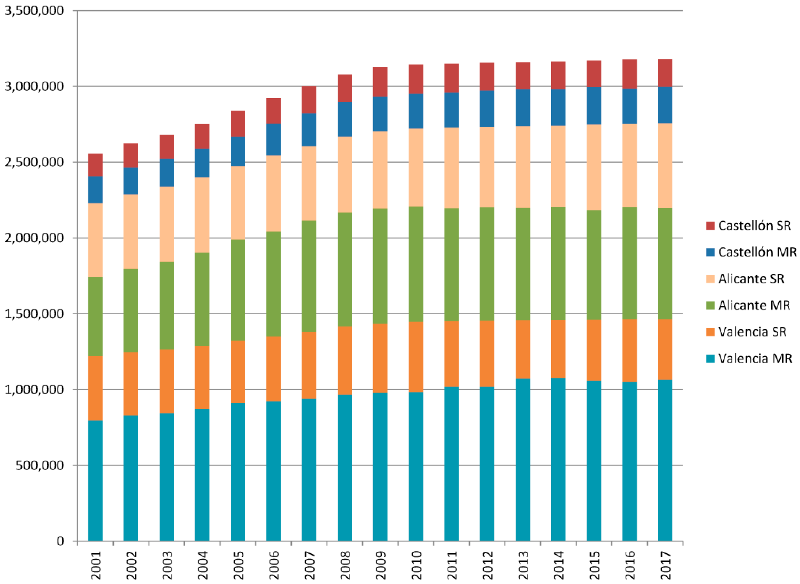
Furthermore, data from the three provinces have demonstrated that, prior to the 2007 crisis, there was an increase in the housing stock of both MR and SR (Figure 1). During the first post-crises decade, the decline of the construction industry resulted in a stabilization of the housing stock numbers to just over three million homes.

The present housing stock scenario in both the central and peripheral provinces of the Valencian Community has resulted in market incentives for a type of housing that is used by owners for a short period of time—in holiday periods, for example, or for short-term residential rentals. Thus, people use “their spare space as an investment” [15]. This has resulted in a greater tourist attraction for the Valencian Community, especially for the province of Alicante. Although it has 170,560 less houses than the province of Valencia (Table 2), the number of SR for most of the year exceeds 161,805 homes.

3. Data Reclassification and Definition of Location Determinants

3.1. Airbnb Data

Airbnb data for the four cities studied were obtained through a third-party provider that “gathers information publicly available on the Airbnb website” [31]. The data for this study was retrieved on the 2 March 2018.

Airbnb’s temporary accommodation listings include metadata related to: listing identification—ID; location—geographic coordinates and information on the country, city, and neighborhood; temporal information—listing creation date; listing characteristics—listing title, description, number of bedrooms, number of bathrooms; pricing data—average pricing rate, deposit, cancelation policy, cleaning fee; user listing evaluation—rating; photographs; maximum number of guests; listing categorization—listing type and property type; among others.

There are sub-categories within the listing type and property type that allow a better definition of the type of accommodation listed. For example, property type includes sub-categories such as apartment, bed and breakfast, boutique hotel, bungalow, camper, dorm, loft, etc.; and a listing type refers to whether the property is completely or partially rented.

In terms of the property type, sub-categories they are sometimes quite vague and inconsistent in their definition. For instance, the difference between property type sub-categories “bed and breakfast” and “entire bed and breakfast” is not evident and sometimes even after analyzing the listings no clarification is possible. Another example of this was found in datasets from Spanish cities which incorrectly included the sub-category “casa particular”—private residence in Spanish—as a property type. These cases occur because when individuals register their properties, they can assign them an existing category or create a new category that does not accurately reflect the type of accommodation. That is why user-generated information from Airbnb datasets is often not classified homogeneously.

Table 3. Proposed groupings and number of Airbnb listings per property type according to frequency.

	Property Type	Frequency	%
Multi-family building	Apartment	6620	33.81
	Entire apartment	6083	31.07
	Private room in apartment	2715	13.87
	Private room in house	399	2.04
	Condominium	396	2.02
	Entire loft	256	1.31
	Private room in bed and breakfast	145	0.74
	Loft	129	0.66
	Other	118	0.60
	Vacation home	93	0.48
	Private room	71	0.36
	Private room in condominium	62	0.32
	Shared room in apartment	38	0.19
	Serviced apartment	34	0.17
	Entire Floor	33	0.17
	Private room in bed & break	29	0.15
	Entire condominium	25	0.13
	Private room in vacation home	20	0.10
	Private room in serviced apartment	8	0.04
	Shared room in house	7	0.04
	Entire bed and breakfast	4	0.02
	Entire vacation home	4	0.02
	Entire serviced apartment	3	0.02
	Shared room in condominium	2	0.01
	Entire floor	1	0.01
	Shared room in guest suite	1	0.01
Single-family building	House	680	3.47
	Entire house	440	2.25
	Entire place	108	0.55
	Entire chalet	36	0.18
	Private room in bungalow	35	0.18
	Entire bungalow	34	0.17
	Entire villa	34	0.17
	Townhouse	28	0.14
	Entire townhouse	26	0.13
	Bungalow	25	0.13
	Chalet	25	0.13
	Villa	24	0.12
	Casa particular	18	0.09
	Private room in casa particular	17	0.09
	Private room in villa	14	0.07
	Private room in chalet	13	0.07
	Private room in townhouse	12	0.06
	Entire cabin	4	0.02
	Shared room in villa	1	0.01
Room	Bed & Breakfast	138	0.70
	Bed & Breakfast	106	0.54
	Private room in guest suite	101	0.52
	Guest suite	51	0.26
	Guesthouse	35	0.18
	Dorm	32	0.16
	Private room in guesthouse	30	0.15
	Hostel	25	0.13
	Private room in dorm	13	0.07
	Private room in hostel	9	0.05
	Private room in loft	7	0.04
	Cabin	6	0.03
	Entire guest suite	5	0.03
	Entire in-law	4	0.02
	Shared room in bed and brea	4	0.02
	Shared room in dorm	4	0.02
	Boutique hotel	1	0.01
	In-law	1	0.01
	Pension (Korea)	1	0.01
	Private room in cabin	1	0.01
	Private room in in-law	1	0.01
	Shared room	1	0.01
	Shared room in bed and breakfast	1	0.01
	Nature lodge	1	0.01
	Shared room in casa particular	1	0.01
Others	Boat	20	0.10
	Camper/RV	7	0.04
	Private room in boat	5	0.03
	Earth House	2	0.01
	Igloo	2	0.01
	Private room in cottage	2	0.01
	Earth house	1	0.01
	Entire boat	1	0.01
	Treehouse	1	0.01
	Total	19,578	100

shows the frequency of accommodation property types found in the case study cities datasets. There were 79 property types initially identified, some of which were duplicated due to typographical errors or slightly different spellings or use of capital letters when referring to the same place. For instance, the “earth house” appears twice “Earth House” and “Earth house”; and, property types “Private room in bed and breakfast” versus “Private room in bed & breakfast” refer to the same kind of accommodation. This matter represents a serious setback for research purposes; therefore, data validation and data pre-processing are required prior to conducting analysis and interpretation.

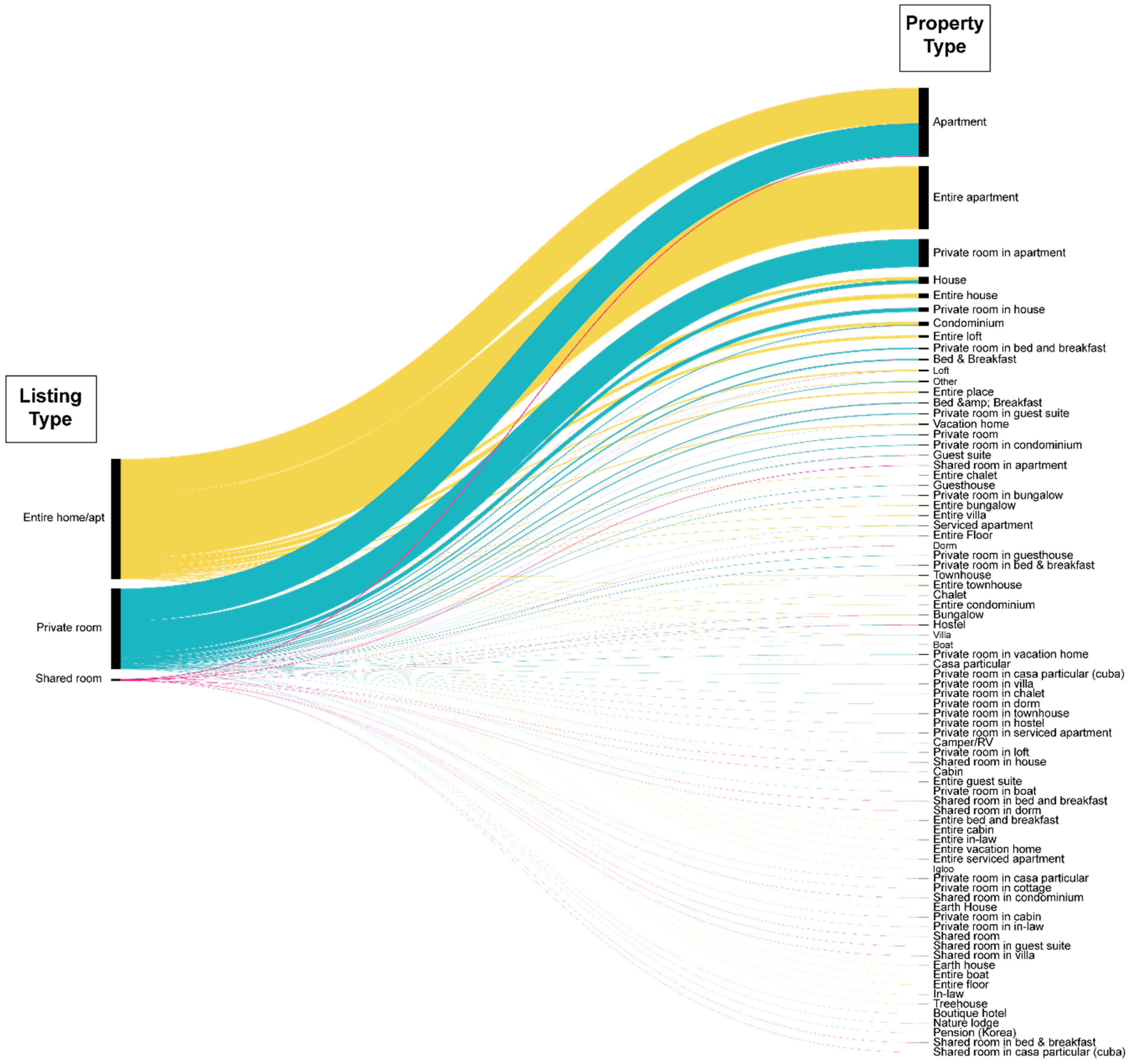
In contrast to the property type, the listing types sub-categories present three listing allocation possibilities: entire house or apartment; private room; or, shared room.

Several combinations can be obtained when analyzing Airbnb listing data, since accommodation listings could be assigned to 79 property types and three listing types (Figure 2).

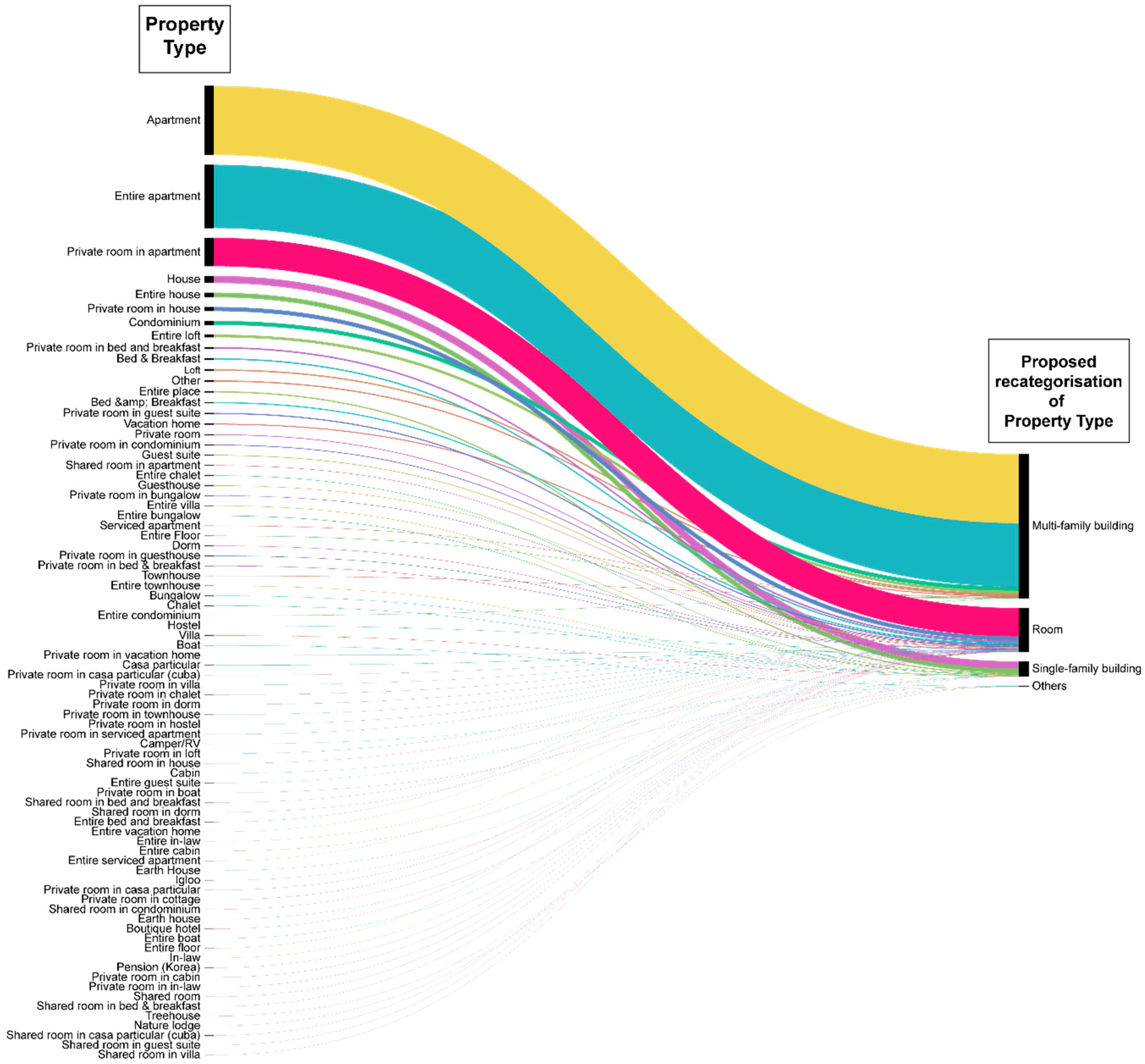
To synthesize the sub-categories on the right-hand side of Figure 2, and refine the datasets, a data re-categorization is proposed for the property types, resulting in four new groups factoring in the accommodations building typology that is more likely to directly affect the price of listings. The first two respond to the building typology of the listing: single-family buildings and multifamily buildings. The third group includes private rooms; and the fourth group, ‘other’, covers non-conventional accommodation listings.

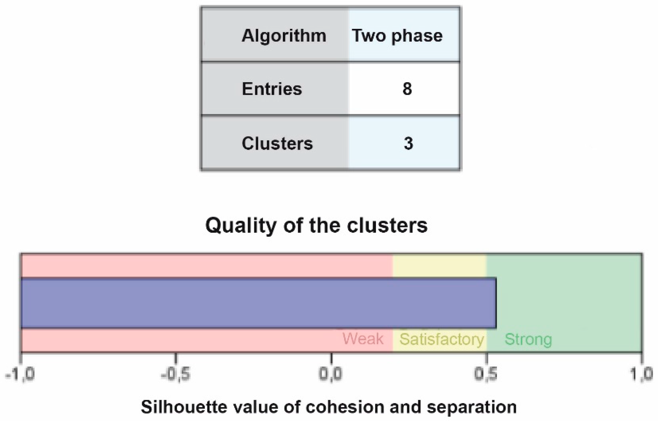
The TwoStep clustering algorithm method is adopted [32] using the SPSS Statistics based program. The clustering calculation of data was performed twice to ensure that the proposed grouping of Airbnb listings is valid. However, it is important to note that only three of the four groups were considered—single-family buildings, multifamily buildings and private rooms. Thus, the results obtained from the calculation comprise three clusters. The fourth group, ‘other’, did not offer a sufficiently high number of listings to be representative (see Table 3) and therefore was excluded from the analysis.

This method offers the benefit of creating clustering models with both, categorical and continuous variables, which is important for carrying out this research because, as shown in

Table 4. Variables considered for the classification.

Numerical Variables		Continuous Variables (Quantity)
	Property type—79 classes	Bathrooms—number
Listing type	Entire home/apartment (0 = N/A, 1 = yes)	Minimum stay—days
	Private room (0 = N/A, 1 = yes)	Daily price—USD
	Shared room (0= N/A, 1 = yes)	Bedrooms—number

N/A = Not Applicable.

, the available data permits the definition of these two types of variables.

For the clustering method, only three of the proposed categories were considered—single-family buildings, multifamily buildings, and private rooms. The fourth category ‘other’ did not offer a sufficiently high number of listings to be representative and therefore was excluded from the analysis.

A summary of the first TwoStep method analysis is presented in Figure 3. As can be observed, the purple bar suggests the validity of the proposed clustering since it falls within the strong portion of the diagram.

The results of the three clusters obtained are presented in

Table 5. Results of the calculations using the TwoStep clustering algorithm.

Airbnb Categories	Variables	Cluster 1	Relevance
Property type	Property_type	Yes, it is a private room in apartment (45.3%) *	1.00
Listing type	Entire_home/apartment	No, it is not an entire home/apartment (100%) *	1.00
	Private_room	Yes, it is a private room (100%) *	1.00
	Shared_room	No, it is not a shared room (100%) *	0.38
	Min_stay	2.03 days **	0.12
	Bathrooms	1.23 units **	0.43
	Daily_price	35.91 USD **	1.00
	Bedrooms	1.10 units **	1.00
		Cluster 2
Property type	Property_type	Yes, it is a house (22.1%) *	1.00
Listing type	Entire_ home/apartment	Yes, it is an entire home/apartment (94%) *	1.00
	Private_room	No, it is not a private room (98.4%) *	1.00
	Shared_room	No, it is not a shared room (95.6%) *	0.38
	Mini_stay	6.76 days **	0.12
	Bathrooms	1.86 units **	0.43
	Daily_price	127.31 USD **	1.00
	Bedrooms	2.30 units **	1.00
		Cluster 3
Property type	Property_type	Yes, it is an apartment (100%) *	1.00
Listing type	Entire_ home/apartment	Yes, it is an entire home/apartment (100%) *	1.00
	Private_room	No, it is not a private room (100%) *	1.00
	Shared_room	No, it is not a shared room (100%) *	0.38
	Min_stay	2.87 days **	0.12
	Bathrooms	1.33 units **	0.43
	Daily_price	95.36 USD **	1.00
	Bedrooms	2.13 units **	1.00

* The most frequent category of the numerical variables. ** The average value of the quantitative variables.

. This table shows that within the clusters obtained, the five most relevant variables are: property_type—property_type; the listing type—Entire home/apartment and Private_room; the daily price—Daily_price; and, the number of bedrooms—Bedrooms.

In the case of the first cluster, it is worth highlighting that in the property type, the subcategory private room in apartment emerges. As for the listing types, this cluster does not include an entire home/apartment or a shared room subcategory. On average, less relevant variables are the daily price and the number of bedrooms—35.91 USD and 1.10 bedrooms respectively. From these characteristics, the obtained cluster category corresponds to private rooms—rooms in a property that cannot be shared with other guests.

As for the second cluster obtained, the relevant property type variable corresponds to the entire home. Moreover, this cluster identifies listing types that refer to entire apartments and neither private rooms nor shared rooms (Table 5). The average daily price and number of bedrooms are the highest among the three clusters obtained—127.31 USD and 2.3 bedrooms, respectively. Taking these characteristics into account, this cluster is grouping entire homes whose building typology refers to single-family dwellings. Table 4 shows that of the three clusters, the second one has more bedrooms and bathrooms and the minimum stay requirement is higher.

The third cluster pinpoints listings that refer to the property type variable apartment as well as the listing type entire home/apartment but neither a shared room nor a private room. The daily price and minimum stay of these listings are less than for the second cluster—single family buildings, but more than the first one—private rooms. From these features it can be assumed that this cluster refers to accommodation in multi-family type buildings which, on average, have 2.13 bedrooms; 1.33 bathrooms and a minimum stay requirement of 2.87 days.

The order in which the variables appear in the matrix is randomly modified and the TwoStep clustering algorithm method is repeated to verify the previous results [32]. The results are analyzed and, as shown in

Table 6. Results of the second calculation using the TwoStep clustering algorithm.

Airbnb categories	Variables	Cluster 1	Relevance
Property type	Property_type	Yes, it is a private room in apartment (45.3%) *	1.00
Listing type	Entire_home/apartment	No, it is not an entire home/apartment (100%) *	1.00
	Private_room	Yes, it is a private room (100%) *	1.00
	Shared_room	No, it is not a shared room (100%) *	0.38
	Min_stay	2.03 days **	0.12
	Bathrooms	1.23 units **	0.43
	Daily_price	35.91 USD **	1.00
	Bedrooms	1.10 units **	1.00
		Cluster 2
Property type	Property_type	Yes, it is a house (22.2%) *	1.00
Listing type	Entire_ home/apartment	Yes, it is an entire home/apartment (93.9%) *	1.00
	Private_room	No, it is not a private room (98.4%) *	1.00
	Shared_room	No, it is not a shared room (95.6%) *	0.38
	Min_stay	6.78 days **	0.12
	Bathrooms	1.66 units **	0.43
	Daily_price	126.52 USD **	1.00
	Bedrooms	2.30 units **	1.00
		Cluster 3
Property type	Property_type	Yes, it is an apartment (100%) *	1.00
Listing type	Entire_ home/apartment	Yes, it is an entire home/apartment (100%) *	1.00
	Private_room	No, it is not a private room (100%) *	1.00
	Shared_room	No, it is not a shared room (100%) *	0.38
	Min_stay	2.87 days **	0.12
	Bathrooms	1.33 units **	0.43
	Daily_price	95.59 USD **	1.00
	Bedrooms	2.14 units **	1.00

* The most frequent category of the numerical variables. ** The average value of the quantitative variables.

, three clusters are defined with very similar characteristics to the ones previously obtained: private room listing type is most relevant in Cluster 1; single-family accommodation listings can be highlighted in the Cluster 2; and listings in multi-family building types are representative in Cluster 3.

The consistency of the variables assigned to the clusters—measurement of inter-rater reliability—is verified through a calculation of the Kappa index. The results obtained are shown in the following

Table 7. Results of the Kappa index calculation.

	Value of K	Asymptotic Standard Error a	Aprox. S b	Aprox. Sig.
Measure of agreement Kappa	0.999	0.000	152.580	0.000
No. of valid cases	13852

a. Null hypothesis is not assumed. b. The asymptotic standard error assumes the null hypothesis.

.

The resulting Kappa coefficient is 0.999. In order to give an interpretation to this coefficient, the tables used by Torres Gordillo and Perera Rodríguez [33], that were first authored by Fleiss, Levin, and Cho Paik [34] and Altman [35] are hereafter presented.

Table 8. Kappa Index interpretation table (Fleiss, 1981).

Value of K	Strength of Agreement
≤0.40	Poor
0.40–0.60	Fair
0.61–0.75	Good
≥0.75	Excellent

and

Table 9. Kappa Index interpretation table (Altman, 1991).

Value of K	Strength of Agreement
≤0.20	Poor
0.21–0.4	Fair
0.41–0.6	Moderate
0.61–0.8	Good
0.81–1.00	Very good

demonstrate that the obtained Kappa value falls within the excellent range, indicating that there is a very good degree of agreement between the obtained clusters and their respectively assigned variables.

Once the clustering criteria is validated, the initial 79 Airbnb group listings are reclassified into the three proposed new categories: single-family buildings; multi-family buildings; and, private rooms. As previously explained, a fourth category covers the non-conventional accommodation types that represent less than 0.5% of the listings.

The recategorization proposed allows a more simplified approach to understanding how the characteristics of the Airbnb properties in a city influence the pricing. Figure 4 and

Table 10. Proposed recategorization Airbnb property types.

Multi-Family Building			Single-Family Building			Room		Others
C	P	CP	C	P	CP	P	CP
Apartment Condominium Entire apartment Entire bed and breakfast Entire condominium Entire Floor Entire loft Entire serviced apartment Entire vacation home Loft Other Private room Private room in apartment Private room in bed and breakfast Private room in condominium Private room in house Private room in serviced apartment Private room in vacation home Serviced apartment Shared room in apartment Shared room in condominium Shared room in guest suite Shared room in house Vacation home			Bungalow Casa particular Chalet Entire bungalow Entire cabin Entire chalet Entire house Entire place Entire townhouse Entire villa House Private room in bungalow Private room in casa particular Private room in chalet Private room in townhouse Private room in villa Shared room in villa Townhouse Villa			Bed & Breakfast Bed & Breakfast Boutique hotel Cabin Dorm Entire guest suite Entire in-Law Guest suite Guesthouse Hostel In-Law Nature lodge Other Pension Private room in cabin Private room in dorm Private room in guest suite Private room in guesthouse Private room in hostel Private room in in-law Private room in loft Shared room Shared room in bed & breakfast Shared room in dorm Nature lodge Shared room in casa particular		Boat Camper/RV Earth House Entire boat Igloo Private room in boat Private room in cottage Treehouse

C: The entire property is rented. P: The property is partially rented—single rooms. CP: The property rents a shared room.

show the result of this recategorization.

3.2. Variables Related to Location

The four case study cities have, to some extent, a touristic character especially given the urban environment of their city centers, where most of the cultural and recreational offer is located. Furthermore, the proximity of these cities to the coast is a common feature that may have an important influence on Airbnb accommodation prices. In consideration of both factors, this study delineates the most touristic area of the city and differentiates between Airbnb accommodation listings that are located in close proximity to the coastline from those that are located towards the most touristic area of the city.

3.2.1. Touristic Area Delineation

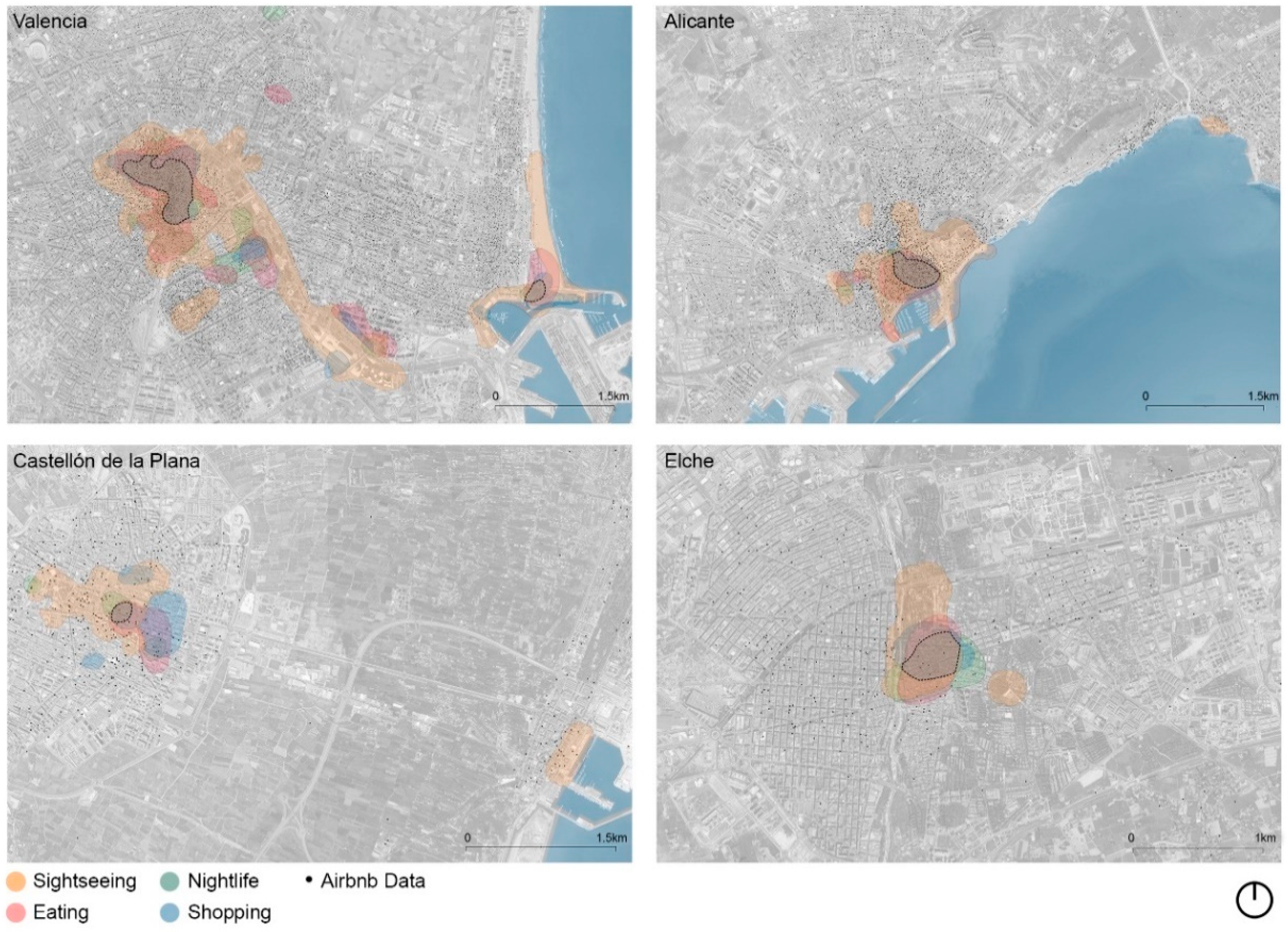
Previous research has addressed the spatial association between the location of Airbnb’s accommodation offer and the city’s touristic hotspots using geolocated social networks information such as that of Panoramio [36]. For this study, Instasights heatmaps [37] have been used as a tool to identify preferred touristic areas of each of the four selected cities. Instasights is a demo website of AVUXI TopPlace Heatmaps service that shows the “most loved areas for main traveler activities” within a city [38]. The heatmaps are built from collected and analyzed “billions of user-generated geotagged signals, regularly indexed across 60+ public sources”. These heatmaps are not downloadable, but access to them is available through the website (www.instasights.com), which visualizes the maps by filtering areas of interest into four categories: most popular eating areas, popular shopping areas, main areas for sightseeing, and favorite nightlife spots. The process for obtaining the curvilinear heatmap shapes of the four categories—layers—is the following. First, a screen shot of each of the four layers is taken and each respective curvilinear heatmap shape is traced onto each city’s cartography using Qgis. Then, the intersection of these four layers is delineated and the resulting polygonal shape is considered the preferred tourist area of each city (Figure 5).

As a result, we obtain four areas with different environmental characteristics—sightseeing, nightlife, eating and shopping—all related to tourism, on which Airbnb listings can be located for each city. These four environmental characteristics are considered as relevant variables for the definition of Airbnb price determinants.

3.2.2. Proximity to the Coastline

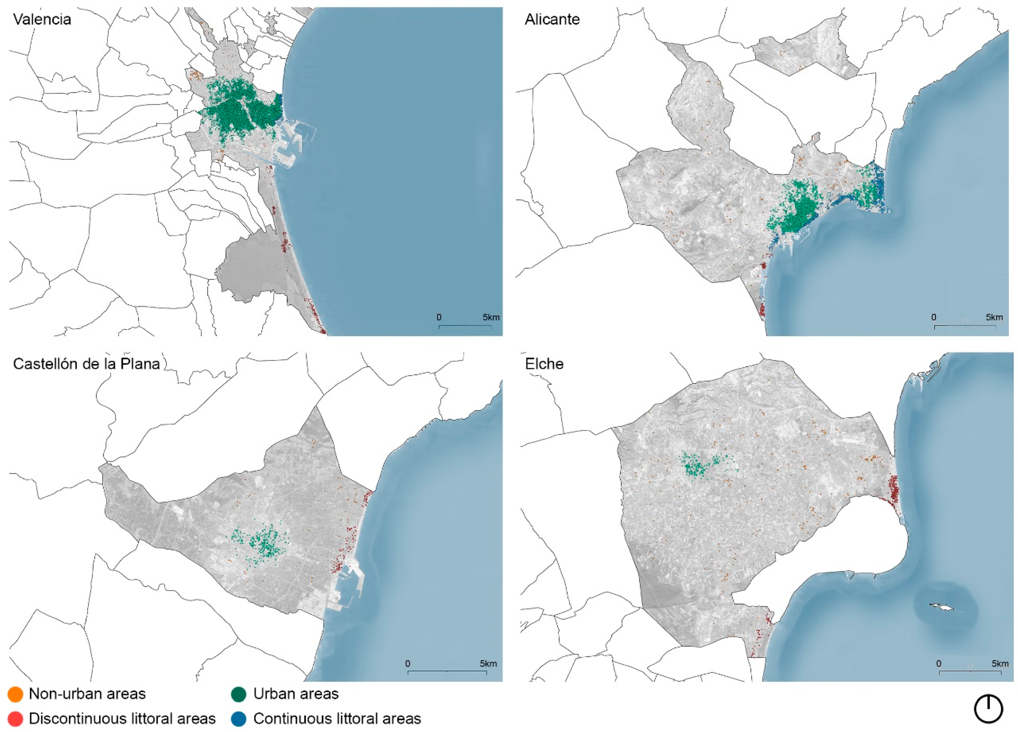
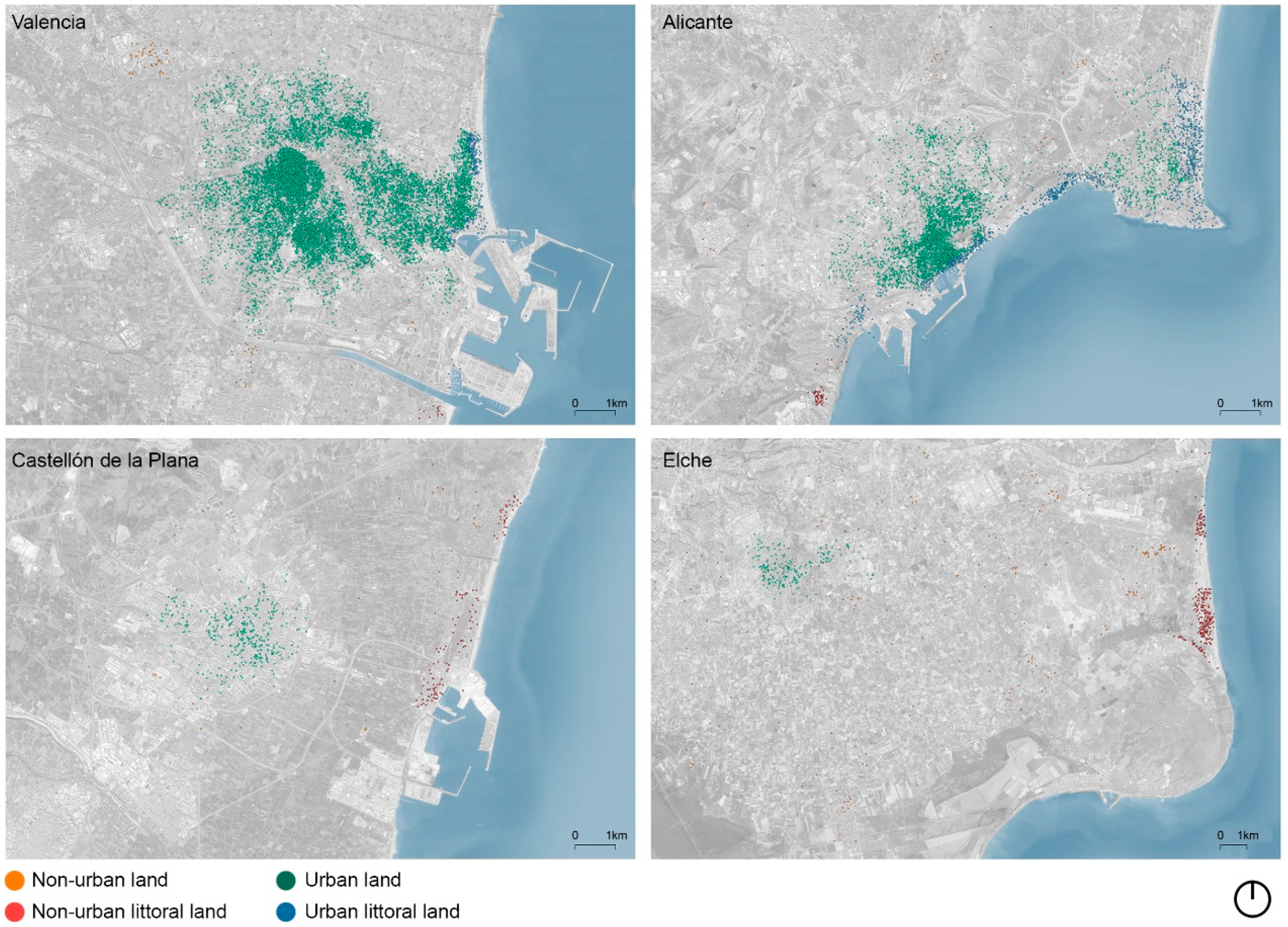
Airbnb datapoints have been differentiated into urban and littoral urban areas in order to identify those listings located within the coastal fringe. Furthermore, it was important to distinguish between the points located within continuous urban land and those in the discontinuous urban land and littoral areas. Presumably continuous urban or littoral areas may be more consolidated with a higher quantity of economic activity on offer and are better connected to other urban areas. Therefore, listings in these locations may differ in price from those located in discontinuous urban areas. Figure 6 and Figure 7 show the differentiation of the listing datapoints into the proposed area types.

4. Data Variables Selection

After perusing and validating Airbnb data, a group of variables was defined considering: (i) Airbnb dataset information; (ii) the variables considered by previous studies; and, (iii) location variables that are highly relevant for the case study selected. The third group of variables introduces both the distance of each Airbnb accommodation listing to the tourist areas of the city and the distance to the coast line.

In total, 5 determinant categories with a total of 26 variables were adopted (

Table 11. Definition of data variables.

Category	Variable Name	Variable Type	Definition
Dependent variable	daily_price	Continuous	Daily price assigned to the property (USD)
Accommodation characteristics	listing_type	Numerical	Identification of offer type, differentiating between room only or complete dwelling: 0 = room only; 1 = complete dwelling
	property_type	Numerical	Identification of property type, differentiating between single-family or multi-family housing: 0 = single-family housing; 1 = multi-family housing
	bathrooms	Continuous	Number of bathrooms available in the property
	max_guests	Continuous	Maximum number of guests permitted
	secu_deposit	Continuous	Deposit requested in USD
	cleaning_fee	Continuous	Housekeeping charge in USD
	cancella_policy	Numerical	Cancellation policy: 1 = flexible; 2 = moderate; 3 = strict; 4 = very strict
	min_stay	Continuous	Minimum rental days required
	bedrooms	Continuous	Number of bedrooms available
Ad and host features	num_photos	Continuous	Number of photos in the advertisement
	ad_online_duration	Continuous	Number of years that the advertisement has been posted online
	rating	Continuous	Guest evaluation score
Environmental characteristics	cat_sightseeing	Numerical	Identification of property location within the four category areas: 1 = Applicable; 0 = Not Applicable (N/A)
	cat_eating	Numerical
	cat_shopping	Numerical
	cat_nightlife	Numerical
Location characteristics	castellon	Numerical	Identification of property location: 1 = Applicable; 0 = Not Applicable (N/A)
	valencia	Numerical
	alicante	Numerical
	elche	Numerical
	con_coastalfringe	Numerical	Identification of property location within a continuous coastal fringe: 1 = Applicable; 0 = N/A
	discon_coastalfringe	Numerical	Identification of property location within a discontinuous coastal fringe: 1 = Applicable; 0 = N/A
	urban_land	Numerical	Identification of property location on urban land or non-urban: 1 = urban land; 0 = non-urban land
	coastal_dist_km	Continuous	Distance (km) from the property to the coast
	inte_cat_dist_km	Continuous	Distance (km) from the property to the intersection of the four category areas

) including:

• The dependent variable, which is the price of the accommodation as advertised on the Airbnb website;
• Accommodation characteristics, which include both the physical definition of the accommodation—the offer type, property type, number of bathrooms, bedrooms available—; and limitations and charges: maximum number of guests allowed, security deposit fee, cleaning fee, cancellation policy, minimum nights of stay;
• Advertisement and host features—number of property photos displayed, how long the property has been advertised online, rating or numeric valuation—;
• Environmental characteristics, accommodation location in relation to the four Instasights tourist layers;
• Location characteristics that distinguish the municipal term in which the accommodation listing is located, the distance from both the coastal fringe and the touristic area.

Table 12. Descriptive statistics.

		Continuous Variables				Numerical Variables
Category	Variable	Average	SD	Min	Max	Codification	Frequency	%
Dependent variable	daily_price	97.71	60.04	11.38	969.13	-
	ln_daily_price	4.45	0.52	2.43	6.88	-
Accommodation characteristics	listing_type	-				0 Room 1 Complete	412 3772	9.8% 90.2%
	property_type	-				0 Single-family 1 Multi-family	316 3868	7.6% 92.4%
	bathrooms	1.38	0.58	0.00	7.00	-
	max_guests	4.65	2.06	1.00	16.00	-
	secu_deposit	240.89	164.52	89.00	4,532.00	-
	cleaning_fee	45.55	26.82	5.00	447.00	-
	cancella_policy	-				1 flexible 2 moderate 3 strict 4 very strict	641 1599 1925 19	15.3% 38.2% 46.0% 0.5%
	min_stay	3.32	13.11	1.00	365.00	-
	bedrooms	2.14	1.09	0.00	9.00	-
Ad and host features	num_photos	23.88	13.71	1.00	131.00	-
	ad_online_duration	2.20	1.38	1.00	6.00	-
	rating	4.56	0.49	1.00	5.00	-
Environmental characteristics	cat_sightseeing	-				0 N/A 1 Applicable	2858 1326	68.3% 31.7%
	cat_eating	-				0 N/A 1 Applicable	3331 853	79.6% 20.4%
	cat_shopping	-				0 N/A 1 Applicable	3542 642	84.7% 15.3%
	cat_nightlife	-				0 N/A 1 Applicable	3665 519	87.6% 12.4%
Location characteristics	valencia	-				0 Alicante 1 Applicable	1265 2919	30.2% 69.8%
	continu_coastline	-				0 N/A 1 Applicable	3735 449	89.3% 10.7%
	discon_coastline	-				0 N/A 1 Applicable	4088 96	97.7% 2.3%
	coastal_dist _km	2.14	1.62	0.00	11.19	-
	inte_cat_dist_ km	1.64	2.52	0.00	20.55	-

Notes: no. of cases 4184.

shows the variables that ultimately have been used in the analysis. The variables castellón and elche, that initially were considered (Table 11), have been removed from subsequent calculations due to the lack of representativeness of the observations in the final dataset. Also, variables in red text turned out to be statistically insignificant. These categories are: property type, min_stay, bedrooms, and cat_nightlife.

5. Method for Identifying the Relation between Accommodation Attributes and Price

This study adopts a multivariable analysis technique which consists of estimating a hedonic price model that is often used in market studies of heterogeneous goods [39]. The method is used for determining and quantifying the relation between Airbnb accommodation attributes and price. To estimate how these characteristics influence price, the model is estimated by using ordinary least squares—OLS—adopting the renowned method of successive steps to select the variables [40].

Although it is a frequently used method in the real estate market, there are some limitations with this approach that must be taken into account. Sirmans et al. [41] highlight that the results obtained with these models are specific to the case study and cannot be generalized to other locations. Chasco Yrigoyen and Sánchez Reyes have also noted that this method is not the most representative if there are relevant extreme values or a high variability [42].

Taking into account the aforementioned limitations, this study adopts the quantile regression method—QRM, whose advantage over the OLS estimation is that the importance of the dependent variable determinants can be explained at any point of the distribution [43]. Thus, the model is less affected since it is not necessary to establish an aleatory perturbation hypothesis. Therefore, the results obtained from the estimation of both models—OLS and QRM, allow identification of the shadow price component of the listing price, which is generated by the accommodation characteristics.

The estimation for these types of models often requires the logarithmic transformation of the dependent variable, the listing price. The literature highlights several reasons as to why the use of semilogarithmic models is rather frequent. For instance, the goodness-of-fit criteria applied to data for avoiding heteroskedasticity and facilitating interpretation of the coefficients. Due to the logarithmic transformation, the goodness-of-fit criteria shows how the dependent variable—the price—presents percentual variables when there are unitary changes of the independent variable [44] (pp. 193–194). Moreover, Sirmans et al. [41] indicate that hedonic models are estimated with logarithmic forms given the great probability that the implicit prices obtained for each characteristic are not the same for all price ranges.

The proposed OLS model is the following:

$$ln\left(P_i\right)=\alpha +{\displaystyle \sum }_{j=1}^n{\beta }_j{X}_{ij}+{\displaystyle \sum }_{k=1}^m{\gamma }_k{D}_{ik}+{\epsilon }_i$$

(1)

where:

• ln (Pi) is the neperian logarithm of daily_price for the property “i”
• α is the fixed component, which is independent from the market.
• β_j is the parameter to be estimated, related to the characteristic “j”.
• X_ij is the continuous variable that considers the characteristic “j” of observation “i”.
• γ_k is the parameter to be estimated, related to the characteristic “k”.
• D_ik is the fictitious variable that considers the characteristic “k” of observation “i”.
• ε_i is the term of the error associated with the observation “i”.

Given the specification of the model, the impact on the price with a change ranging from 0 to 1 in a dummy variable, while keeping all other independent variables constant, can be calculated using the expression (2), as Kennedy suggests [45]

$$\widehat{p}=100\left[exp\left(\widehat{c}-\frac{1}{2}\widehat{V}\left(\widehat{c}\right)\right)-1\right]$$

(2)

The percentage change on the dummy variable is estimated as $\widehat{p}$, $\widehat{V}\left(\widehat{c}\right)$. It is the variance estimation of $\widehat{c}$ in the OLS model, calculated as the square of the standard deviation of the coefficient: $\widehat{\mathrm{V}}\left(\widehat{\mathrm{c}}\right)=\widehat{{\mathrm{SE}}^2}$.

The quantile regression method does not require the fulfillment of certain criteria as in the case of the OLS model. The QRM allows controlling non-linearity; non-normality due to asymmetries and outliers; and heteroskedasticity [42]. OLS models are based on the conditional mean of the dependent variable, given certain values of the predictor variables, but do not provide information for other conditional quantiles of the dependent variable, whereas QRM allows modeling different conditional quantiles of the dependent variable, overcoming the limitations of OLS models. Thus, it is possible to estimate the implicit value of each accommodation characteristic for different price ranges—or quantiles—as they may vary [41]. Then, the impact of each characteristic, depending on the sales price ranges, can be estimated. As suggested by [46,47], a QRM can be defined using a multiple linear regression model as

$$Y_i=X_i{\beta }_{\theta }+u_{\theta i}$$

(3)

where

• Y_i is the dependent variable
• X_i is the matrix of independent variables
• β_θ is the vector of parameters to be estimated for quantile θ
• u_θi is the aleatory perturbation that corresponds to quantile θ.

As explained by Koenker and Bassett [46] (p. 38), in this regression model, quantiles θ are defined for the dependent variable Y_i, given the X_i dependent variables, where Quant(Y_i|X_i) = X_iβ_θ. Each quantile regression θ, with 0 < θ < 1, is defined as the solution to the minimization problem, which is solved with a simplex linear programming model

$$\underset{\beta \in R^k}{\min }\left\{{\displaystyle \sum }_{i\in \left\{i:Y_i\ge X_i\beta \right\}}\theta \left|Y_i-X_i{\beta }_{\theta }\right|+{\displaystyle \sum }_{i\in \left\{i:Y_i<X_i\beta \right\}}\left(1-\theta \right)\left|Y_i-X_i{\beta }_{\theta }\right|\right\}$$

(4)

The parameter estimation for the QRM is formulated through minimization of the mean absolute deviation with asymmetric weights, whereas in the OLS is obtained by minimizing the sum of squared residuals. The median regression is a particular case of the quantile regression where θ = 0.5, being the only case in which the weighs are symmetric.

The quantile regression has been estimated using the statistical package R “quantreg”—version 5.36 [48]. The algorithmic method used to compute the fit is the modified version of Barrodale and Roberts [49], and is described in detail by Koenker and d’Orey [50,51]. The goodness-of-fit of quantile models has been calculated from the absolute deviations using the pseudo-R¹ [52]. It is useful to compare quantile models; however, they are not comparable to the determination coefficient obtained through OLS as it is based on the variance of the square deviations. The pseudo-R¹ is obtained as 1 minus the ratio between the sum of absolute deviations in the fully parameterized models and the sum of absolute deviations in the null (non-conditional) quantile model.

6. Results

The results of the OLS model (1) are shown in

Table 13. OLS regression model.

	(Constant)	2.777 *** (0.054)
Accommodation characteristics	listing_type	0.563 *** (0.018)
	bathrooms	0.157 *** (0.010)
	max_guests	0.061 *** (0.003)
	secu_deposit	0.0002 *** (0.00003)
	cleaning_fee	0.005 *** (0.0002)
	cancella_policy	0.032 *** (0.007)
Ad and host features	num_photos	0.001 *** (0.0003)
	ad_online_duration	0.013 *** (0.004)
	rating	0.024 * (0.010)
Environmental characteristics	cat_sightseeing	0.152 *** (0.015)
	cat_eating	0.054 * (0.022)
	cat_shopping	0.048 * (0.022)
Location characteristics	alicante	Reference
	valencia	0.165 *** (0.013)
	con_coastalfringe	0.109 *** (0.019)
	discon_coastalfringe	−0.115 * (0.048)
	coastal_dist_km	−0.027 *** (0.004)
	inte_cat_dist_km	0.013 *** (0.003)
Statistical significance *** p < 0.001, ** p < 0.01, * p < 0.05
	R²	0.641
	adj. R²	0.639
	Std. Error	0.31116
	F (sig.)	437.329 (0.000)
	DW	1.737

Notes: dependent variable Neperian logarithm daily_price.

. If analyzed by categories, the results demonstrate that, within the first group of variables—accommodation characteristics—all estimated determinants are positive, which means that they are all variables that have an influence on Airbnb accommodation prices. The most important variables of this group are the daily price—daily_price and the type of accommodation offer—listing_type. Since this dummy variable distinguishes whether the listing is a single room or an entire dwelling, the obtained value demonstrated that when renting an entire dwelling, the price of the property increases by 75.6% when compared to that of a single room. Having an additional bathroom—bathrooms—increases the price by 16%. The rest of the accommodation category characteristics have less of an effect on the price, with listing prices increase beyond 5% only for the variable maximum number of lodging guests—max_guests.

With respect to the second category—ad and host features—the variable with a greater influence on Airbnb price is the one that corresponds to the guest listing rating—rating.

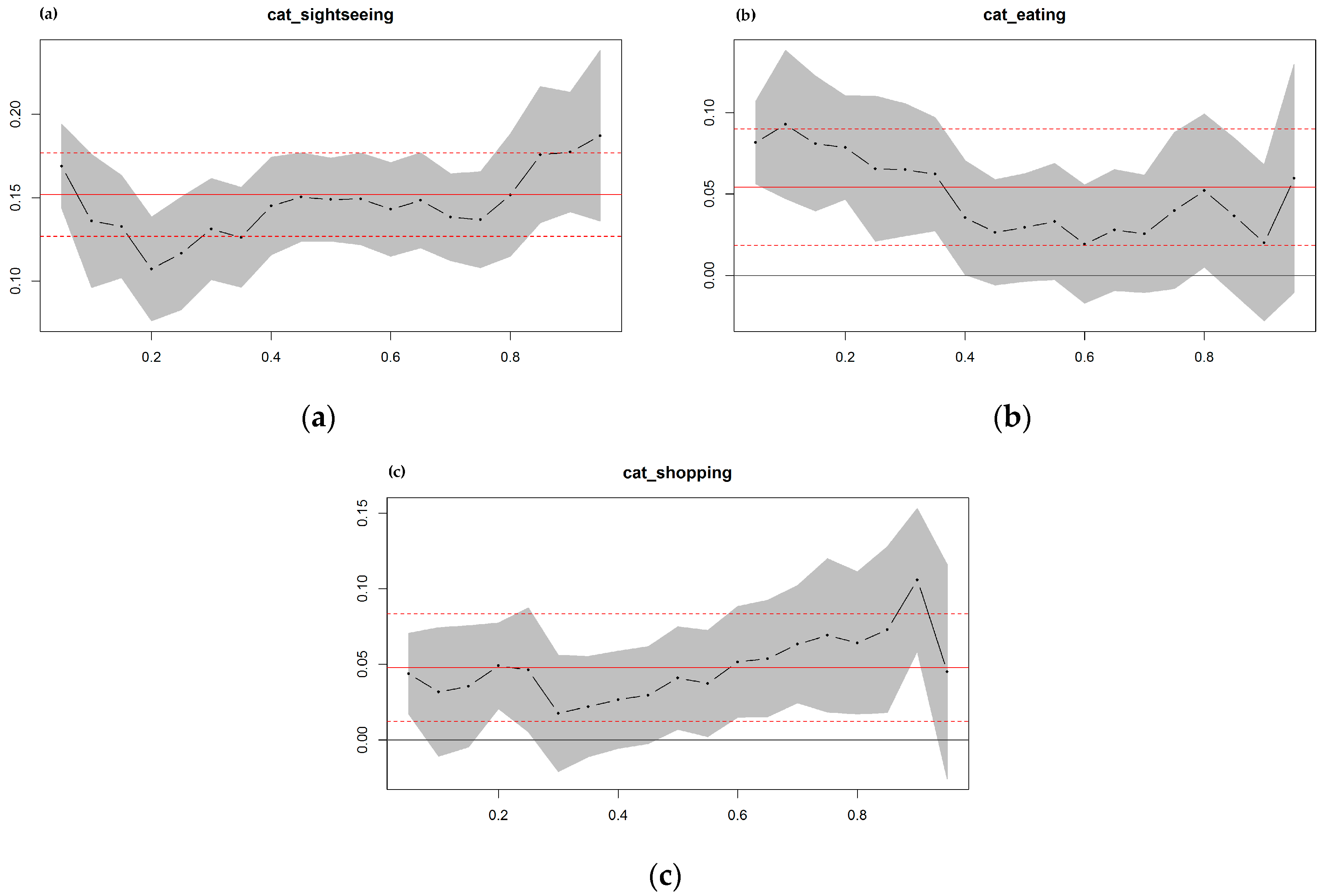
All variables in the third category—environmental characteristics—are relevant given their positive values. Results show that those listings within or closer to the defined sightseeing tourist area—cat_sightseeing—have the greatest impact on price, causing a 16% increase. The areas falling within the eating and shopping categories—cat_eating and cat_shopping—show a similar effect but produce a smaller 5% increase.

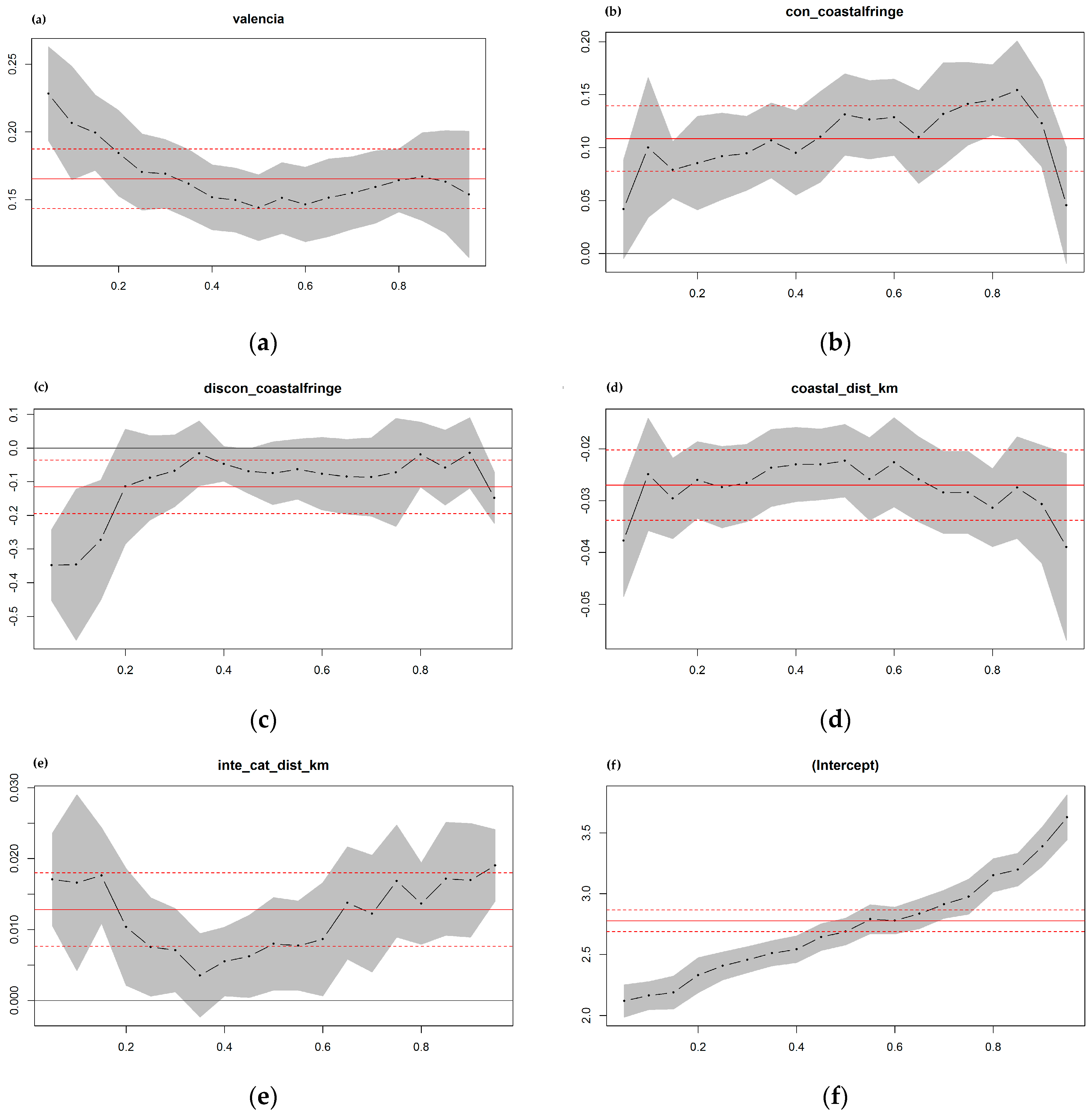
The last category—location characteristics—include variables with both a positive and negative impact on price. Listings for properties located in Valencia increase by 18% compared to the rest of the listings, especially in comparison to other properties with the same characteristics but located in Alicante—alicante and valencia variables. Furthermore, if the accommodation is located in the continuous littoral coastal fringe—con_coastalfringe—price increases by 11.5%. However, if the listing is located in the discontinuous littoral coastal fringe area—discon_coastalfringe—the price decreases by approximately the same percentage. Moreover, for each kilometer from the coastline, the price of the accommodation decreases by 3%—coastal_dist_km.

The last variable considered within the location characteristics—inte_cat_dist_km—is worth highlighting because the findings show that for each kilometer from the defined touristic area, accommodation price is 1.3% more expensive.

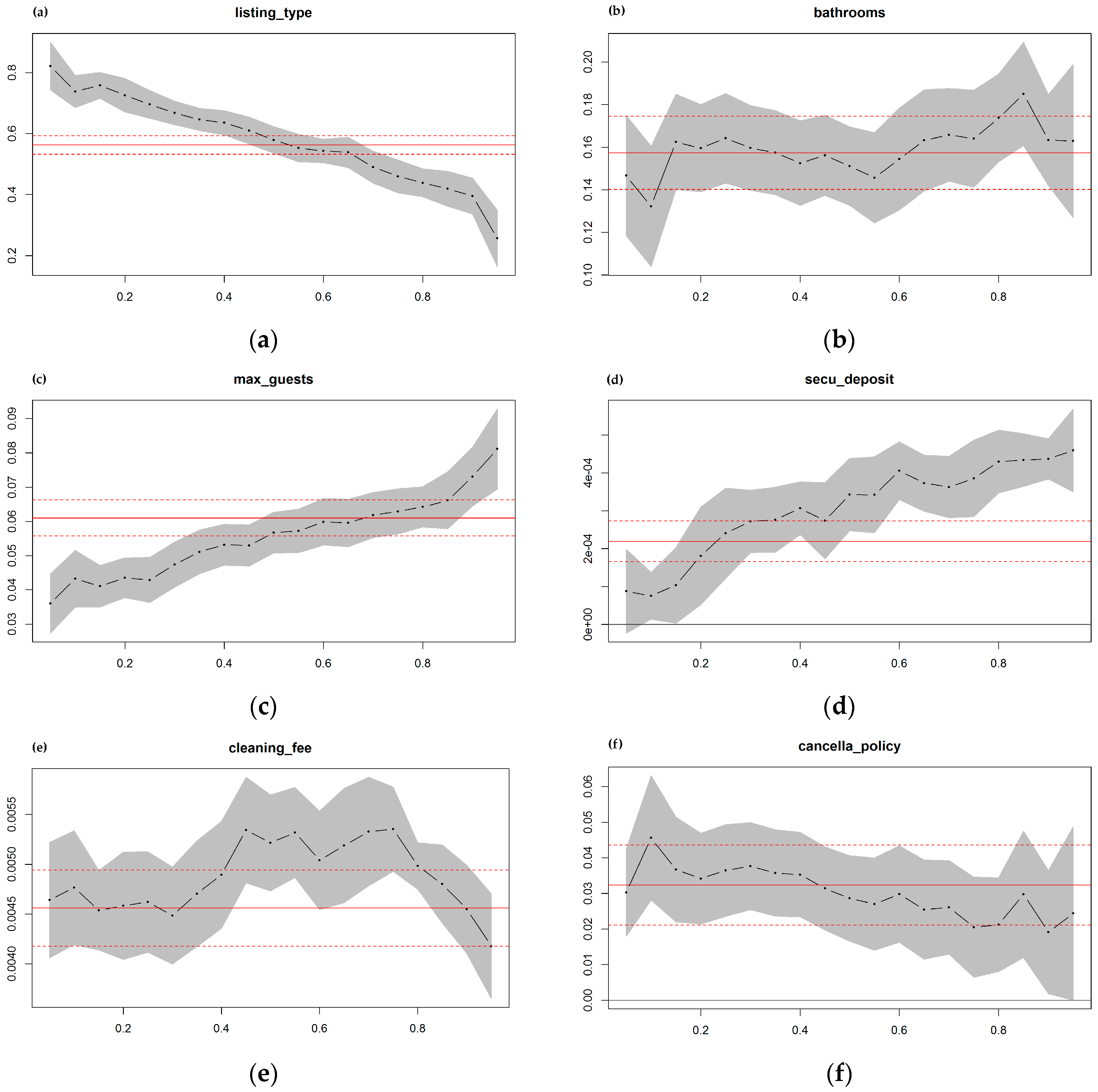
The results of the quantile model (3) are shown in

Table 14. Quantile regression models: coefficients and standard errors, QR 0.10, 0.25, 0.50, 0.75, 0.90.

		Model 1 QR 0.10	Model 2 QR 0.25	Model 3 QR 0.50	Model 4 QR 0.75	Model 5 QR 0.90
	(Constant)	2.164 *** (0.069)	2.407 *** (0.070)	2.688 *** (0.066)	2.975 *** (0.087)	3.388 *** (0.098)
Accommodation characteristics	listing_type	0.738 *** (0.032)	0.696 *** (0.028)	0.579 *** (0.027)	0.460 *** (0.033)	0.395 *** (0.036)
	bathrooms	0.132 *** (0.017)	0.164 *** (0.013)	0.151 *** (0.011)	0.164 *** (0.014)	0.163 *** (0.013)
	max_guests	0.043 *** (0.005)	0.043 *** (0.004)	0.057 *** (0.004)	0.063 *** (0.004)	0.073 *** (0.005)
	secu_deposit	0.0001 * (0.00004)	0.0002 *** (0.0001)	0.0003 *** (0.00006)	0.0004 *** (0.0001)	0.0004 *** (0.00003)
	cleaning_fee	0.005 *** (0.0003)	0.005 *** (0.0003)	0.005 *** (0.0003)	0.005 *** (0.0003)	0.005 *** (0.0003)
	cancella_policy	0.046 *** (0.011)	0.036 *** (0.008)	0.029 *** (0.007)	0.021 * (0.009)	0.019 (0.011)
Ad and host features	num_photos	0.003 *** (0.001)	0.001 ** (0.0004)	0.0009 * (0.0003)	0.001 ** (0.0005)	0.001 (0.001)
	ad_online_duration	−0.00002 (0.006)	0.008 (0.005)	0.017 *** (0.004)	0.016 *** (0.004)	0.005 (0.005)
	rating	0.058 *** (0.011)	0.055 *** (0.013)	0.037 ** (0.012)	0.027 (0.016)	−0.008 (0.019)
Environmental characteristics	cat_sightseeing	0.136 *** (0.024)	0.117 *** (0.021)	0.149 *** (0.015)	0.137 *** (0.018)	0.177 *** (0.022)
	cat_eating	0.093 *** (0.028)	0.066 * (0.027)	0.029 (0.020)	0.040 (0.029)	0.020 (0.029)
	cat_shopping	0.032 (0.026)	0.046 (0.025)	0.041 * (0.021)	0.069 * (0.031)	0.106 *** (0.029)
	valencia	0.207 *** (0.025)	0.170 *** (0.017)	0.144 *** (0.015)	0.159 *** (0.016)	0.163 *** (0.023)
	con_coastalfringe	0.100 * (0.040)	0.092 *** (0.025)	0.131 *** (0.023)	0.141 *** (0.024)	0.123 *** (0.025)
	discon_coastalfringe	−0.346 * (0.136)	−0.089 (0.076)	−0.075 (0.056)	−0.072 (0.097)	−0.015 (0.063)
	coastal_dist_km	−0.025 *** (0.007)	−0.027 *** (0.005)	−0.022 *** (0.004)	−0.028 *** (0.005)	−0.031 *** (0.007)
	inte_cat_dist_km	0.017 * (0.008)	0.008 (0.004)	0.008 * (0.004)	0.017 *** (0.005)	0.017 *** (0.005)
	pseudo-R1	0.479	0.415	0.378	0.378	0.397

Notes: dependent variable Neperian logarithm daily_price. Statistical significance *** p < 0.001, ** p < 0.01, * p < 0.05; standard errors in parentheses; pseudo-R¹ see [52].

. The relevance of the variable listing type (a) reduces as prices increase, as can be observed in the “Accommodation Characteristics” category (Figure 8). Given that this variable discriminates between the type of offer—complete dwelling or single room, the quantiles of the highest prices only comprises complete dwellings and, consequently, the distinction between the two typologies becomes irrelevant. In

Table A1. Quantile regression models: t-test and statistical significance, QR 0.10, 0.25, 0.50, 0.75, 0.90.

		Model 1 QR 0.10	Model 2 QR 0.25	Model 3 QR 0.50	Model 4 QR 0.75	Model 5 QR 0.90
	(Constant)	31.197 (0.000)	34.578 (0.000)	40.234 (0.000)	34.204 (0.000)	34.415 (0.000)
Accommodation characteristics	listing_type	23.020 (0.000)	24.944 (0.000)	21.801 (0.000)	14.047 (0.000)	11.032 (0.000)
	bathrooms	7.703 (0.000)	12.824 (0.000)	13.462 (0.000)	11.849 (0.000)	12.568 (0.000)
	max_guests	8.605 (0.000)	10.714 (0.000)	15.716 (0.000)	15.624 (0.000)	13.980 (0.000)
	secu_deposit	2.007 (0.045)	3.317 (0.001)	5.899 (0.000)	6.287 (0.000)	13.473 (0.000)
	cleaning_fee	13.710 (0.000)	15.019 (0.000)	17.751 (0.000)	20.779 (0.000)	16.872 (0.000)
	cancella_policy	4.296 (0.000)	4.657 (0.000)	3.926 (0.000)	2.402 (0.016)	1.820 (0.069)
Ad and host features	num_photos	4.253 (0.000)	2.953 (0.003)	2.329 (0.020)	2.711 (0.007)	1.122 (0.262)
	ad_online_duration	−0.003 (0.998)	1.631 (0.103)	4.298 (0.000)	4.141 (0.000)	1.017 (0.309)
	rating	5.460 (0.000)	4.322 (0.000)	3.000 (0.003)	1.670 (0.095)	−0.410 (0.682)
Environmental characteristics	cat_sightseeing	5.607 (0.000)	5.684 (0.000)	9.852 (0.000)	7.816 (0.000)	8.125 (0.000)
	cat_eating	3.353 (0.001)	2.424 (0.015)	1.467 (0.142)	1.367 (0.172)	0.690 (0.490)
	cat_shopping	1.228 (0.220)	1.859 (0.063)	1.986 (0.047)	2.243 (0.025)	3.693 (0.000)
	valencia	8.132 (0.000)	9.966 (0.000)	9.744 (0.000)	9.790 (0.000)	7.104 (0.000)
	con_coastalfringe	2.493 (0.013)	3.712 (0.000)	5.627 (0.000)	5.963 (0.000)	4.926 (0.000)
	discon_coastalfringe	−2.543 (0.011)	−1.162 (0.245)	−1.327 (0.185)	−0.744 (0.457)	−0.231 (0.817)
	coastal_dist_km	−3.786 (0.000)	−5.754 (0.000)	−5.247 (0.000)	–5.897 (0.000)	−4.451 (0.000)
	inte_cat_dist_km	2.201 (0.028)	1.791 (0.073)	2.011 (0.044)	3.505 (0.000)	3.481 (0.001)

Notes: dependent variable Neperian logarithm daily_price; in parentheses the statistical significance of the t-test.

—Appendix A—the t-test values are provided and their statistical significance.

Figure 8, Figure 9, Figure 10 and Figure 11 present a graphical representation of the quantile regression. The variation in the slope of each regression coefficient can be observed for different values of the dependent variable—quantiles. The quantiles and the regression coefficient values are represented by the horizontal and the vertical axes, respectively. The black dash-dot line represents the estimation of the quantile regression coefficient. The gray area represents the 95% confidence interval of the coefficients. The solid red horizontal line represents the OLS coefficient. The red dashed line represents the 95% confidence interval of the OLS estimation. The coefficient is considered statistically insignificant in those cases where the coefficient confidence interval reaches zero—gray horizontal line—for a given quantile.

According to Figure 8 the influence of the variable bathrooms on price quantiles (b) shows some stability, mainly between quartiles 0.20 and 0.80. Therefore, this variable’s impact—bathrooms—is practically similar for low and high prices. The maximum number of guests’ variable—max_guests—(c), shows a positive trend, having greater impact on higher prices than on lower ones. This same effect can be observed with the security deposit variable—secu_deposit—(d), although its influence on all price ranges is not significant. The cleaning fee variable—cleaning_fee—(e) also shows insignificant impact. It mostly affects prices of quantiles 0.40 to 0.80. The last variable in the category, the cancellation policy—cancella_policy—(f), has less influence on higher priced listings.

Regarding the variable related to the listing’s number of pictures (a)—num_photos, within the category of advertisement and host features, the impact on prices is practically insignificant (Figure 9), having a similar effect on all quantiles. However, more impact has been recognized for the advertisement online duration time variable (b)—ad_online_duration. The price impact increases between quantiles 0.20 and 0.50 and, from that point, it stabilizes until it reaches quantile 0.80. As for the last variable of this category, the guest rating impact on price (c)—rating—decreases as the rental price increases. From quantile 0.75, the variable is no longer significant.

As for the category of environmental characteristics, Figure 10 shows that the first variable related to sightseeing—cat_sightseeing—(a) impacts price most, with a similar effect for quantiles 0.40 and 0.80. The second variable—cat_eating—(b), is only significant up to quantile 0.4; whilst the third variable—cat_shopping—(c), is significant up to quantile 0.50, meaning that the impact of these variables is greater as the rental price increases.

The results from the location characteristics category (Figure 11), indicate that if the property is in Valencia city—valencia—(a), there is a decline in the effect on price between quantiles 0.20 and 0.50. From that point onwards, the effect on price of a listing located in Valencia moderately increases up to quantile 0.80. At this point, the effect reaches a similar value to the one obtained for quantile 0.30. The second variable—con_coastalfringe—(b) shows a positive impact on the price. Moreover, the listing location within the continuous coastal strip has a greater impact on the price of expensive properties. The third variable—discon_coastalfringe—(c), is only significant up to quantile 0.20. When considering the distance from the property to the coastline—coastal_dist_km—(d), a similar effect is indicated between quantiles 0.20 and 0.60 but intensity diminishes in the highly priced listings—between the quartiles 0.60 and 0.80. Finally, the distance of properties to the touristic area polygon, —inte_cat_dist_km—(e), has a positive effect that increases from quantile 0.40, having a greater impact on highly priced listings. Thus, the greater the distance from the touristic area polygon, the higher the listing price.

7. Discussion

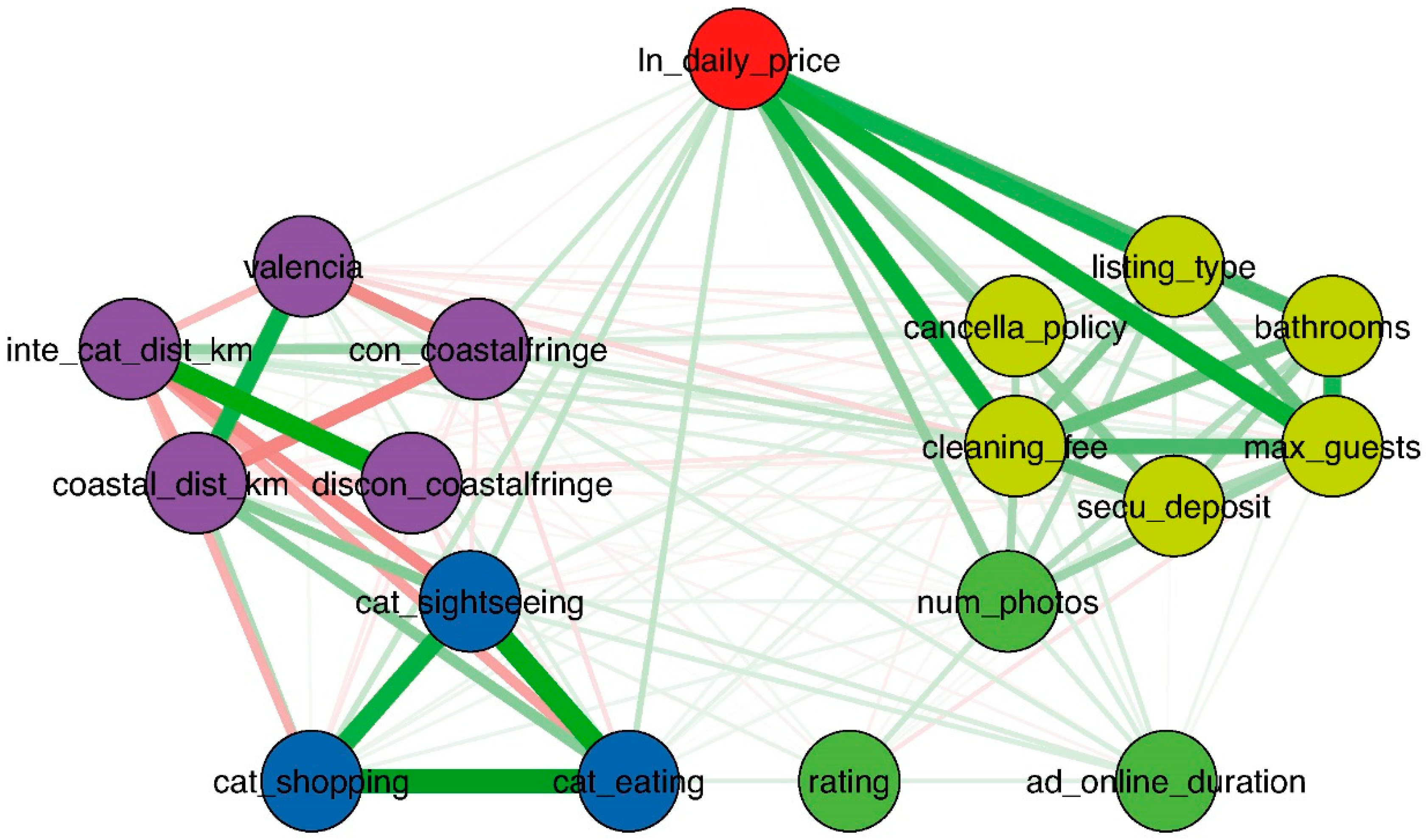
The results of this study demonstrate how the property listing characteristics impact rental prices (Figure 12).

In relation to the OLS estimation, the accommodation characteristics category indicates that the property size has a significant impact on price, which is indirectly affected by the variables listing_type, bathrooms, and max_guests. For instance, on average, an extra bathroom increases the price by 15.7%, and an extra guest by 6.1%. This concurs with the literature [24,53,54,55,56,57].

The results obtained from the quantile regression are in line with those of the OLS estimation. That is, the maximum number of guests’ variable—max_guests—has an increasing effect on price for all quantiles. Moreover, the effect increases for the most expensive properties. The impact of the number of bathrooms—bathrooms—is constant for almost all quantiles. However, the influence is more pronounced for the most expensive listings—quantile 0.80.

Previous research [23,24,58,59] recognizes the importance of the advertisement and host features category in accordance with the results of the OLS estimation. These features include: the number of property listing photos; the online publication date; and, the guest rating, which is crucial. It can be assumed that owners of well rated properties exploit this differentiation to increase rental prices. Furthermore, results from the quantile regression in this matter point in the same direction. However, the impact of guest rating in this method diminishes as listing price increases, having minimum impact in quartiles close to 0.80.

As for the environmental characteristics’ category, the location of properties in areas with a good concentration of shopping and food services—cat_sightseeing, cat_shopping, and cat_eating—has a positive influence on the rental price. If the accommodation is located in any of these areas, listing prices increase by almost 15% for properties located within cat_sightseeing and by 5% for dwellings located in popular areas for cat_shopping and cat_eating. Thus, the quantile regression model estimates that the variable cat_sightseeing has the greatest impact, maintaining a similar intensity between quantiles 0.40 and 0.80. The price quantiles of the other two variables, cat_shopping and cat_eating, are insignificant.

The location characteristics category indicates that daily prices in Valencia are 16.5% higher than those of Alicante. In this respect, the results of the quantile regression confirmed the findings, showing that listing properties located in Valencia are more expensive than those in Alicante. However, the impact of this determinant over Valencia dwellings diminishes, reaching prices of quantile 0.50 and maintaining similar magnitudes along prices of upper quantiles.

Additionally, if the listing is located within the littoral fringe, the price increases by 10.9% for listings in the continuous urban littoral land—con_coastalfringe. However, the price decreases by 11.5% for listings in the discontinuous urban littoral land—discon_coastalfringe. This differential is due to the fact that the continuous urban littoral land is more consolidated and, therefore, has more economic activity and is better connected to other central urban areas. These characteristics are highlighted by the proposed model that on average estimates net price differences of 22.4%. Furthermore, the property price decreases by 2.7% per kilometer from the coastline—coastal_dis_km. The property’s distance from the continuous coastal fringe has a more significant effect on properties with high listing prices, whilst the distance from the coastline has a similar effect between quantiles 0.20 and 0.60, decreasing for higher priced listings—quantile 0.80.

As for the last variable related to the location characteristics—inte_cat_dist_km—this study has demonstrated that for each kilometer from the accommodation to the delimited touristic area, the listing price increases by 1.3%. Furthermore, the tourist area identified happens to be in the city center for all studied cases. Thus, contrary to what literature suggests, the case study cities do not meet the initial hypothesis that stated that the closer to the city center, the more expensive Airbnb accommodation listing.

In this regard, pprevious research has studied the impact on price of the distance from the city center [24,60,61,62,63] to the tourist accommodation, finding that prices decrease as distance increases. However, this study did not use the city center as a reference point because often city centers are not necessarily the location of the highest concentration of diverse urban and economic activities that may be of interest to tourists. Hence, it was important to consider determinants such as environmental and location characteristic categories that could be transferred to other case studies. These variables introduce a novel approach to identifying price determinants. The model considers the effect on price of disaggregated characteristics that introduce information related to the property location and the surrounding urban environment.

The accommodation characteristics adopted acknowledge how different urban areas with Airbnb listings are interrelated in terms of the vacation rental market and economic development. A breakthrough in the rental market has occurred and it is having a huge impact on rental prices; however, it is also attracting more tourists who contribute to the sustainability of local trade by contributing to a better distributed economic development of the city.

8. Conclusions

This research adds to the current debate on the range of factors that may influence Airbnb accommodation prices. Specifically, five groups of determinants are considered in the study: the daily price of the listing, accommodation attributes, advertisement and host features, tourism-related environmental characteristics, and the listing’s location. However, from these initial groups, the results indicate that the accommodation prices are essentially driven by the following three considerations: the physical characteristics—the what; the factors which impact user perception—the why; and, the location—the where.

Relatively few studies have investigated the listing location determinant. Thus far, research has included the location of Airbnb listings in relation to nearest landmark [22] and tourist attractions [36], the city center in general [24]; hotels [64] and, key central infrastructures, such as the city’s convention center [22]. The present study provides a novel approach to understanding a location’s impact on the Airbnb listing price. This involves identifying and quantifying the spatial relationships between the location of Airbnb accommodation and the most highly touristic area of the city, as well as the coastline.

Some degree of distance from the most relevant tourist area is one of the main variables that positively affects Airbnb accommodation prices, according to this study of four Spanish Mediterranean Arc cities. The literature, thus far, has indicated that accommodation price increases in locations closest to the city center, whereas the results of this study indicate the contrary. Accommodation price increases as distance increases from the delimited tourist area, which is in the historic city center, thereby enriching by providing an exception to the literature in this field.

This study offers three main methodological contributions to the literature: (i) the validation and reclassification of Airbnb data for research purposes that to the authors’ knowledge has been given little coverage, if any; (ii) the identification of touristic activity areas; (iii) obtaining the variables that influence Airbnb accommodation prices by using a multivariable analysis technique and adopting both the ordinary least squares and quantile regression model methods to estimate how Airbnb characteristics influence listing prices.

All three methodological approaches are reproducible to other case studies, specifically, the proposed Airbnb data reclassification and the definition of the city’s touristic areas. As for the distance to the coastline variable, this evidently would provide relevant results for territories similar to those considered in this case study.

The transformation of second residence homes into short-term tourist rental accommodation can, if properly managed, positively impact neighbourhoods and cities in the Valencian community [65]. These dwellings provide the potential for exploiting a business model such as Airbnb—that pioneers the management of this type of business [15] and caters to a new tourist profile that demands rental housing. Furthermore, as a good amount of Airbnb’s offers are in locations outside the most relevant tourist areas of the four cities studied, arguably this would have a great impact on economic and urban sustainability matters in terms of consumption patterns and dwelling under-utilization.

As for consumption patterns—both spatial and temporal—have been transformed by this sharing economy service [66] as opposed to incrementing purely the economic activity of certain areas [64]. This along with the host recommendations for local leisure and other services [11] results in an integration of the tourist into local life. Thus, revenue inflows from tourism become better distributed throughout the city, positively affecting urban spaces that may be outside exclusively touristic areas. As a result, areas that might seem to be lacking urban activity can benefit from a mix of local and tourist population, especially areas where secondary housing is predominant over primary housing that lack urban activity during low season. With the presence of Airbnb accommodation in these areas, increase in demand may encourage commercial activities to remain open throughout the year. Therefore, areas with Airbnb listings could become catalysts for more evenly distributed urban activity, which in turn could attract property developers which will enhance the urban environment.

Dwelling under-utilization is key to sharing platforms such as Airbnb [30] since this service “leverages existing housing inventory” [64], whereas hotels require local zoning to be in place. This suggests that the empty-property syndrome caused by the Spanish real-estate bubble may be reverted by this type of accommodation service. Owners of second residencies are now able to make profit from unused properties. In this respect, future research, beyond the scope of this study, could benefit from introducing data from other sources of information such as Fotocasa and Idealista, which are web platforms for medium-to-long-stay accommodation rentals. This would further inform studies on how much of the existing secondary housing stock is being activated by these short-, medium-, and long-term rental services.

References

- Hamari, J.; Sjöklint, M.; Ukkonen, A. The sharing economy: Why people participate in collaborative consumption. J. Assoc. Inf. Sci. Technol. 2015, 67, 2047–2059. [Google Scholar] [CrossRef]
- Tussyadiah, I.P.; Pesonen, J. Impacts of Peer-to-Peer Accommodation Use on Travel Patterns. J. Travel Res. 2016. [Google Scholar] [CrossRef]
- Fang, B.; Ye, Q.; Law, R. Effect of sharing economy on tourism industry employment. Ann. Tour. Res. 2016, 57, 264–267. [Google Scholar] [CrossRef]
- Chesky, B.; Gebbia, J.; Blecharczyk, N. 10 Years of Community. Available online: https://press.airbnb.com/10-years-of-community/ (accessed on 12 October 2018).
- Wang, C.; Jeong, M. What makes you choose Airbnb again? An examination of users’ perceptions toward the website and their stay. Int. J. Hosp. Manag. 2018, 74. [Google Scholar] [CrossRef]
- Ert, E.; Fleischer, A.; Magen, N. Trust and reputation in the sharing economy: The role of personal photos in Airbnb. Tour. Manag. 2016, 55, 62–73. [Google Scholar] [CrossRef]
- Airbnb. Airbnb and the Rise of Millennial Travel. Economistas, 22 November 2016. [Google Scholar]
- Guttentag, D. Airbnb: Disruptive innovation and the rise of an informal tourism accommodation sector. Curr. Issues Tour. 2013, 18. [Google Scholar] [CrossRef]
- Stors, N.; Kagermeier, A. Motives for Using Airbnb in Metropolitan Tourism—Why do People Sleep in the Bed of a Stranger? Reg. Mag. 2015, 299, 17–19. [Google Scholar] [CrossRef]
- Chen, Y.; Xie, K.L. Consumer valuation of Airbnb listings: A hedonic pricing approach. Int. J. Contemp. Hosp. Manag. 2017, 29, 2405–2424. [Google Scholar] [CrossRef]
- Díaz Armas, R.J.; García Rodríguez, F.J.; Gutiérrez Taño, D. Airbnb como nuevo modelo de negocio disruptivo en la empresa turística: Un análisis de su potencial competitivo a partir de las opiniones de los usuarios. In Proceedings of the XVIII Congreso AECIT. Turismo: Liderazgo, Innovación y Emprendimiento, Benidorm, Spain, 26–28 November 2014. [Google Scholar]
- Liang, S.; Schuckert, M.; Law, R.; Chen, C.-C. Be a “Superhost”: The importance of badge systems for peer-to-peer rental accommodations. Tour. Manag. 2017, 60. [Google Scholar] [CrossRef]
- Prothero, A.; Dobscha, S.; Freund, J.; Kilbourne, W.E.; Luchs, M.G.; Ozanne, L.K.; Thøgersen, J. Sustainable Consumption: Opportunities for Consumer Research and Public Policy. J. Public Policy Mark. 2011, 30, 31–38. [Google Scholar] [CrossRef]
- Danielle Sacks The Sharing Economy. Available online: https://www.fastcompany.com/1747551/sharing-economy (accessed on 18 October 2018).
- Botsman, R.; Rogers, R. What’s Mine Is Yours: The Rise of Collaborative Consumption; HarperCollins Business: New York City, USA, 2010; ISBN 9780874216561. [Google Scholar]
- Priceonomics Airbnb vs Hotels: A Price Comparison. Available online: https://priceonomics.com/hotels/ (accessed on 15 October 2018).
- Lawler, R. Airbnb: Our Guests Stay Longer and Spend More Than Hotel Guests, Contributing $56M to the San Francisco Economy. Available online: https://techcrunch.com/2012/11/09/airbnb-research-data-dump/?guccounter=1 (accessed on 10 October 2018).
- Porges, S. The Airbnb Effect: Bringing Life To Quiet Neighborhoods. Available online: https://www.forbes.com/sites/sethporges/2013/01/23/the-airbnb-effect-bringing-life-to-quiet-neighborhoods/#560623fb5a86 (accessed on 15 October 2018).
- Hung, W.T.; Shang, J.K.; Wang, F.C. Pricing determinants in the hotel industry: Quantile regression analysis. Int. J. Hosp. Manag. 2010, 29, 378–384. [Google Scholar] [CrossRef]
- Wong, K.K.F.; Kim, S. Exploring the differences in hotel guests’ willingness-to-pay for hotel rooms with different views. Int. J. Hosp. Tour. Adm. 2012, 13, 6–93. [Google Scholar] [CrossRef]
- Yelkur, R.; Nêveda Dacosta, M.M. Differential pricing and segmentation on the Internet: The case of hotels. Manag. Decis. 2001, 39, 252–261. [Google Scholar] [CrossRef]
- Zhang, Z.; Chen, R.J.C.; Han, L.D.; Yang, L. Key factors affecting the price of Airbnb listings: A geographically weighted approach. Sustainability 2017, 9, 1635. [Google Scholar] [CrossRef]
- Ikkala, T.; Lampinen, A. Defining the price of hospitality: Networked hospitality exchange via Airbnb. In Proceedings of the 17th ACM Conference on Computer Supported Cooperative Work & Social Computing (CSCW Companion 2014), Baltimore, MD, USA, 15–19 February 2014; pp. 173–176. [Google Scholar]
- Wang, D.; Nicolau, J.L. Price determinants of sharing economy based accommodation rental: A study of listings from 33 cities on Airbnb.com. Int. J. Hosp. Manag. 2017. [Google Scholar] [CrossRef]
- Li, Y.; Pan, Q.; Yang, T.; Guo, L. Reasonable price recommendation on Airbnb using Multi-Scale clustering. In Proceedings of the 2016 35th Chinese Control Conference, Chengdu, China, 27–29 July 2016; pp. 7038–7041. [Google Scholar]
- Tang, E.; Sangani, K. Neighborhood and Price Prediction for San Francisco Airbnb Listings. Available online: http://cs229.stanford.edu/proj2015/236_report.pdf (accessed on 15 October 2018).
- INE Instituto Nacional de Estadística. Available online: http://www.ine.es/ (accessed on 10 October 2018).
- Font Arellano, A. The Explosion of the City: Territorial Transformations in the South Europe Urban Regions; Ministerio de Vivienda: Madrid, Spain, 2006; ISBN 978-84-96387-25-6. [Google Scholar]
- Ministerio de Fomento Vivienda. Available online: https://www.fomento.gob.es/vivienda (accessed on 17 October 2018).
- Frenken, K.; Schor, J. Putting the sharing economy into perspective. Environ. Innov. Soc. Trans. 2017, 23, 3–10. [Google Scholar] [CrossRef]
- AirDNA Short-Term Rental Data Methodology—The AI and science behind AirDNA. Available online: https://www.airdna.co/methodology (accessed on 28 August 2018).
- Rubio-Hurtado, M.-J.; Vilà-Baños, R. El análisis de conglomerados bietápico o en dos fases con SPSS. Rev. Innov. Recerca Educ. 2016, 10, 118–126. [Google Scholar] [CrossRef]
- Torres Gordillo, J.J.; Perera Rodríguez, V.H. Cálculo de la fiabilidad y concordancia entre codificadores de un sistema de categorías para el estudio del foro online en e-learning. Rev. Investig. Educ. 2009, 27, 89–103. [Google Scholar]
- Fleiss, J.L.; Levin, B.; Cho Paik, M. Statistical Methods for Rates and Proportions; Wiley: Hayfork, CA, USA, 1981; ISBN 0471064289. [Google Scholar]
- Altman, D.G. Practical Statistics for Medical Research; Chapman: New York, NY, USA, 1991; ISBN 0-412-27630-5. [Google Scholar]
- Gutiérrez, J.; García-Palomares, J.C.; Romanillos, G.; Salas-Olmedo, M.H. The eruption of Airbnb in tourist cities: Comparing spatial patterns of hotels and peer-to-peer accommodation in Barcelona. Tour. Manag. 2017, 62, 278–291. [Google Scholar] [CrossRef] [Green Version]
- AVUXI Ltd. What Are AVUXI TopPlace Heat Maps? Available online: http://support.avuxi.com/support/what-are-avuxi-geopopularity-heat-maps (accessed on 3 October 2018).
- AVUXI LTD InstaSights. Available online: https://www.instasights.com (accessed on 1 August 2018).
- Lancaster, K.J. A New Approach to Consumer Theory Author. J. Polit. Econ. 1966, 74, 132–157. [Google Scholar] [CrossRef]
- Álvarez Cáceres, R. Estadística Multivariante y No Paramétrica con SPSS: Aplicación a las Ciencias de la Salud; Ediciones Díaz de Santos: Madrid, Spain, 1995; ISBN 978-8479781804. [Google Scholar]
- Sirmans, S.; Macpherson, D.; Zietz, E. The composition of hedonic pricing models. J. Real Estate Lit. 2005, 13, 1–44. [Google Scholar]
- Yrigoyen, C.C.; Sánchez Reyes, B. E Prezo Da Vivenda En Madrid. Rev. Galega Econ. 2012, 21, 277–296. [Google Scholar]
- Zietz, J.; Zietz, E.N.; Sirmans, G.S. Determinants of house prices: A quantile regression approach. J. Real Estate Financ. Econ. 2008, 37, 317–333. [Google Scholar] [CrossRef]
- Kain, J.F.; Quigley, J.M. Housing Markets and Racial Discrimination: A Microeconomic Analysis; Urban and Regional Studies; Univ Microfilms Inc.: Ann Arbor, MI, USA, 1975; ISBN 978-0-87014-270-3. [Google Scholar]
- Kennedy, P.E. Estimation with correctly interpreted dummy variables in semilogarithmic equations. Am. Econ. Rev. 1981, 71, 801. [Google Scholar] [CrossRef]
- Koenker, R.; Bassett, G. Regression Quantiles. Econometrica 1978, 46, 33–50. [Google Scholar] [CrossRef]
- Koenker, R. Quantile Regression; Cambridge University Press: New York, NY, USA, 2005; ISBN 9780521845731. [Google Scholar]
- Koenker, R. R Package ‘Quantreg’ 2018. Available online: https://CRAN.R-project.org/package=quantreg (accessed on 5 September 2018).
- Barroda, I.; Roberts, F.D.K. Solution of an overdetermined system of equations in the l1 norm [F4]. Commun. ACM 1974, 17, 319–320. [Google Scholar] [CrossRef]
- Koenker, R.; D’Orey, V. Remark AS R92: A Remark on Algorithm AS 229: Computing Dual Regression Quantiles and Regression Rank Scores. J. R. Stat. Soc. 1994, 43, 410–414. [Google Scholar] [CrossRef]
- Koenker, R.; D’Orey, V. Algorithm AS 229: Computing Regression Quantiles. J. R. Stat. Soc. 1987, 36, 383–393. [Google Scholar] [CrossRef]
- Koenker, R.; Machado, J.A.F. Goodness of Fit and related inference processes for quantile regression. J. Am. Stat. Assoc. 1999, 94, 1296–1310. [Google Scholar] [CrossRef]
- Kaya, A.; Atan, M. Determination of the Factors That Affect House Prices in Turkey by Using Hedonic Pricing Model. J. Bus. Econ. Financ. 2014, 3, 313–327. [Google Scholar]
- Carlos, J.; Velásquez, H.; Agudelo, J. Infraestructura pública y precios de vivienda: Una aplicación de regresión geográficamente ponderada en el contexto de precios hedónicos. Ecos Econ. 2011, 15, 95–122. [Google Scholar]
- Quispe Villafuerte, A. Una aplicación del modelo de precios hedónicos al mercado de viviendas en Lima metropolitana. Rev. Econ. 2017, 9, 85–122. [Google Scholar]
- Marmolejo, C. The incidence of the energy rating on residential values: An analysis for the multifamily market in Barcelona. Inf. Constr. 2016, 68, e156. [Google Scholar] [CrossRef]
- Lama Santos, F.A. Determinación de las Cualidades de Valor en la Valoración de Bienes Inmuebles. La Influencia del Nivel Socioeconómico en la Valoración de la Vivienda. Ph.D. Thesis, Universitat Politècnica de València, Valencia, Spain, 2017. [Google Scholar]
- Gutt, D.; Herrmann, P. Sharing means caring? Hosts’ price reaction to rating visibility. In ECIS 2015 Research-in-Progress Papers; AIS Electronic Library (AISeL): Münster, Germany, 2015; Volume 54. [Google Scholar]
- Li, J.; Moreno, A.; Zhang, D.J. Agent Pricing Behavior in the Sharing Economy: Evidence from Airbnb. SSRN Electron. J. 2015. [Google Scholar] [CrossRef]
- Bull, A.O. Pricing a motel’s location. Int. J. Contemp. Hosp. Manag. 1994, 6, 10–15. [Google Scholar] [CrossRef]
- Chen, C.F.; Rothschild, R. An application of hedonic pricing analysis to the case of hotel rooms in Taipei. Tour. Econ. 2010, 16, 685–694. [Google Scholar] [CrossRef]
- Lee, S.K.; Jang, S.C. Premium or discount in hotel room rates? the dual effects of a central downtown location. Cornell Hosp. Q. 2012, 53, 165–173. [Google Scholar] [CrossRef]
- Zhang, H.; Zhang, J.; Lu, S.; Cheng, S.; Zhang, J. Modeling hotel room price with geographically weighted regression. Int. J. Hosp. Manag. 2011, 30, 1036–1043. [Google Scholar] [CrossRef]
- Zervas, G.; Proserpio, D.; Byers, J. The rise of the sharing economy: Estimating the impact of Airbnb on the hotel industry. J. Mark. Res. 2017, 54, 687–705. [Google Scholar] [CrossRef]
- Moreno Izquierdo, L.; Ramón Rodríguez, A.; Such Devesa, M.J. Turismo colaborativo: ¿Está Airbnb transformando el sector del alojamiento? Economistas 2016, 150, 107–119. [Google Scholar]
- Perles Ribes, J.; Moreno Izquierdo, L.; Ramón Rodríguez, A.; Such Devesa, M. The Rental Prices of the Apartments under the New Tourist Environment: A Hedonic Price Model Applied to the Spanish Sun-and-Beach Destinations. Economies 2018, 6, 23. [Google Scholar] [CrossRef]
Figure 1.
Amount of main residence (MR) and second homes (SR) in the provinces of Alicante, Castellón, and Valencia. Source: Spanish Ministry of Development [29].
Figure 2.
Distribution of property types per listing type.
Figure 3.
Clustering model summary.
Figure 4.
Recategorization of Airbnb data into four groups: multi-family, single-family, single room, and others.
Figure 5.
Areas with different environmental characteristics: sightseeing, nightlife, eating and shopping. The outlined polygon represents the intersection of these four areas.
Figure 6.
Municipal area of the four case study cities differentiating urban from littoral urban areas—within the coastal fringe; and continuous and discontinuous urban land.
Figure 7.
Zoomed-in view and its spatial relation to the coastal area.
Figure 8.
Quantile regression model, accommodation characteristics category: (a) listing_type, (b) bathrooms, (c) max_guests, (d) secu_deposit, (e) cleaning_fee and (f) cancella_policy.
Figure 9.
Quantile regression model, ad and host features category: (a) num_photos, (b) ad_online_duration and (c) rating.
Figure 10.
Quantile regression model, environmental characteristics category: (a) cat_sightseeing, (b) cat_eating and (c) cat_shopping.
Figure 11.
Quantile regression model, location characteristics category: (a) valencia, (b) con_coastalfringe, (c) discon_coastalfringe, (d) coastal_dist_km, (e) inte_cat_dist_km and (f) intercept.
Figure 12.
Correlation between the adopted property listing characteristics—variables—and Airbnb prices.