Built Environment and Parking Availability: Impacts on Car Ownership and Use

Abstract

Along with urbanization and economic development, the number of private cars has increased rapidly in recent years in China, which contributes to concerns about traffic congestion, hard parking, energy consumption, and emissions. This study aims to investigate the joint effect of built environment and parking availability on car ownership and use based on a household travel survey conducted in Changchun, China. The binary logistic model was first employed to investigate the determinants of the car ownership in Changchun. Next, this study examined the potential impacts of the built environment and parking availability on car use for the journey to work. The result shows that built environment and parking availability can be both significantly associated with car ownership and use after controlling for the socio-economic characteristics. Moreover, in contrast with the model ignoring the parking availability, the model for car use considering the joint effect fit the data better. The results indicate that car dependency depends on the joint effect of the built environment and parking availability. These results suggest that transit-oriented urban expansion and compact land use can contribute to reducing car commuting. Meanwhile, parking restrictions at both trip start and end would be effective for sustainable transport because parking oversupply could encourage more car dependency.

1. Introduction

In China, concerns about transportation energy consumption and emissions force the government to promote sustainable urbanization and combat the economic, environmental, energy, and safety issues that go with rapid motorization [1]. According to an official report, the number of private cars in China has reached 100 times what it was in 1990. The rapid growth of car ownership and use contributes to most of the concerns [2]. Therefore, promotion of urban sustainable transportation through reducing car ownership and use is of significant importance for energy conservation and emissions reduction.

A variety of literature has identified a wide range of factors influencing car ownership and use, such as socio-economic characteristics, parking availability, and management policies [3,4,5,6,7,8,9]. In addition, there is a growing body of research that focuses on the influence of the built environment on car dependency [10,11,12,13,14,15]. However, there are still some major gaps that need to be filled. First, few studies focus on the influence of the built environment on car ownership and use in developing countries, especially in small and mid-sized cities. Thus, the existing studies conducted in western countries can provide few policy implications for the small and mid-sized cities in China, where car ownership and use are still growing constantly. Taking Changchun as a case, the number of private cars has reached 1.23 million in 2013, a 251% increase from 2008. Second, previous studies rarely take into account intentions of households without cars in purchasing one. However, in small and mid-sized cities in China, many households still cannot afford to purchase a car [16]. Therefore, the intentions of households without cars will be associated with the private car number in the future. More importantly, existing studies exploring the influence of built environment on car dependency rarely take into account the parking availability, which may lead to mis-understanding of the role the built environment plays [17]. Finally, apart from residential built environment, the built environment at job locations can also influence the commuting mode choice. To the best of our knowledge, however, few efforts have been made to account for this influence [13,18].

This paper aims to fill the gaps simultaneously by exploring the joint effect of the built environment and parking availability at both residence and workplace on car dependency. The remainder of this paper is organized as follows. The following section is a review of existing literature. The third section presents the data and method used in this study. Then, the following section discusses the results. The final section provides the conclusions and recommendations for future studies.

2. Literature Review

2.1. The Impacts of Built Environment on Travel Behavior

Built environment, residents’ daily activities, and spatial locations are important terms that can potentially determine travel behavior [17,19,20]. A growing body of literature has investigated the influence of the built environment on car ownership and use [3,12,21]. However, previous studies have returned debatable conclusions. For instance, Naess [19] used Nordic cities as a case to explore the influence of urban form on travel behavior and found that density had a significant influence on travel behavior at the significant level of 95% (Coeff. = −0.60). Conversely, Ewing and Cervero [22] analyzed existing literature that examines the interaction between the built environment and travel behavior and concluded that population and employment density were not significantly associated with household vehicle miles traveled (VMT) (Coeff. = −0.05).

Built environment consists of some measurements, including diversity, density, distance to transit, and destination accessibility, which have been summarized as “D variables”. Land use mixture is a key component representing diversity, which has received much attention [23,24,25]. For instance, Acker and Witlox [25] treated car ownership as a mediating variable between built environment and car use and confirmed that land use mixture had a significant influence on car use at the significance level of 99% (Coeff. = −0.023). However, some researchers have claimed that the built environment has little influence on car dependency. Distance to transit is another key factor, that plays an important role in influencing travel behavior due to the “Transit Metropolis” program in China [26,27]. Li et al. [3] implemented regression models to investigate the influence of transit accessibility and found that non-work car dependency of the residents living near metro stations were influenced by the built environment significantly at the significant level of 99% (Coeff. = −1.018). Density is usually quantified by the residential and employment density. Ding et al. [12] investigated the influence of the residential and employment density on car ownership and travel distance. The results indicate that households living in areas with lower residential density tend to have a higher probability of owning cars at the significance level of 95% (Coeff. = −0.103). In addition, employment density is found to have a significant influence on car ownership and travel distance at the significance level of 95%. Design is a component which is usually represented by street network connection, intersection density or block size. Hong et al. [28] implemented a Bayesian model and found that the intersection density was negatively related (−0.24) with non-work related VMT at the significance level of 95%. This means that people living in areas with lower intersection density tend to drive more than others for non-work purpose. Destination accessibility is an element representing the location, which is proven to have a negative influence on VMT [12,29,30].

However, it is still unclear about the link between the built environment and car dependency in China due to the fact that few studies are conducted in Chinese cities. On the other hand, rapid urbanization has provided a new insight into the link between the built environment characteristics and commuting mode choice in many Chinese cities.

2.2. The Impacts of Parking Facilities on Car Ownership and Use

The majority of car ownership and use studies mention the effects of parking facilities on travel behavior, directly or indirectly [9,17]. The effects of workplace parking on mode choice for the journey to work have been explored in many studies [31,32,33,34]. For instance, Christiansen [17] explored the influence of workplace parking availability on commuting mode choice and found that the influence of parking regulations at the workplace on car use was significant at the significance level of 95% (Coeff. = −0.205). It is an effective way for employers to reduce the probability of driving alone by providing parking discounts for ride-sharers [32]. Liu et al. [35] employed a structural equation model to investigate how parking interplayed with the built environment and affected car commuting in Shenzhen. Rye et al. [36] used Edinburgh as a case to explore the influence of workplace parking on commuting mode choice and the results indicate that controlled parking zones can reduce the car use. However, few studies have focused on the effects of origin parking availability on car ownership and use until recently [35]. Some studies show that the influence of parking restraints at the origin of a trip is also important for car use [8,9,17]. For instance, Weinberger [37] used a generalized linear model to predict the proportion of residents who drive to work considering the parking supply in neighborhoods. Guo [9] measured the parking supply for 770 households in New York City region using Google Street View and found that residential parking supply significantly determined the household car ownership and use decision. Guo [8] investigated the effect of home parking convenience on household car usage and found that home parking limitations helped to reduce households' car usage. Previous studies have produced mixed results about the effects of parking at the origin and destination of a trip. Some studies suggest that the residential parking supply could affect car ownership and use because a car would be parked for most of its lifetime [38]. However, others would argue that car dependency is primarily affected by the travel demand budget constraints rather than parking regulations [39].

2.3. Other Factors Influencing Car Ownership and Use

Apart from built environment and parking availability, there are other factors influencing car ownership and use. Additionally, compared with built environment and parking availability, some researchers have realized that the socio-economic characteristics are more important factors [11,40,41]. Especially in China, the economic factor could be a determinant because many households still cannot afford to purchase a car [16].

Income is one of the most important factors and it has been well explored in previous studies [42,43]. Some researchers have confirmed that income is a determine of car dependency in China [41], although some researchers argue that household income has little influence on VMT [24]. Household size and structure are both factors that could influence car ownership and use. Different household structures can generate different car travel demand, such as education and healthcare purposes [23].

Different from the studies conducted in western countries, Hukou system is a term that could influence the car ownership and use in China. Hukou system is a special mechanism preventing people living in rural areas moving into cities [44]. In addition, it also prevents many migrant workers from some social welfare. Therefore, whether the household has local Hukou can be a determinant of car ownership and use.

Apart from the aforementioned characteristics, attitude and preference characteristics have received more attention recently as self-selection effects [41,45,46,47,48]. A variety of outcomes from self-selection effect have been empirically examined, ranging from travel model choice [47,49,50,51] to transportation energy consumption and emissions [41,45]. With rapid urbanization, car ownership is still growing constantly in small and mid-sized cities in China. In order to reduce car dependency in Chinese cities, the Chinese government has invested a huge amount in their public transport systems. Therefore, transit accessibility is a term that needs to be considered in China.

Based on our literature review, we have developed two research hypotheses: (1) socio-economic characteristic, built environment, and parking availability collectively have significant impacts on car ownership and use decision; (2) it will lead to a bias estimation for the impacts if parking availability effects are not taken into account. To support these hypotheses, this study employed four binary logistic models to explore the joint effect of socio-economic characteristic, built environment, and parking availability on car ownership and use decision.

3. Research Design

3.1. City Context of Changchun

We focused on Changchun in this study, which is a mid-sized city in Northeast China. Changchun is the capital of Jilin Province. The study region is shown as Figure 1. The population of Changchun has reached 3.63 million and Changchun has an area of 16,410 km² until 2012 [2]. At the end of 2012, it had two metro lines covering 47.6 km. Moreover, Changchun has been chosen as a member of the “Transit Metropolis” program in 2013, which is a program proposed by the Ministry of Transportation in China, aiming to promote sustainable transportation as a way of reducing car use [52]. However, the number of cars is still growing rapidly. The number of cars has reached 1.23 million in 2013, which is 3.51 times as that in 2008 [53]. A series of problems related to car dependency such as traffic congestion, energy shortage, and air pollution have become urgent to solve.

Many studies have explored the influence of built environment and parking availability respectively. However, few studies focus on their joint effects. Therefore, these studies might mis-understand the influence of the built environment and parking availability due to the deviation caused by variable omission. This study aims to fill the gaps and provide preferences for similar cities in China.

3.2. Data and Variables

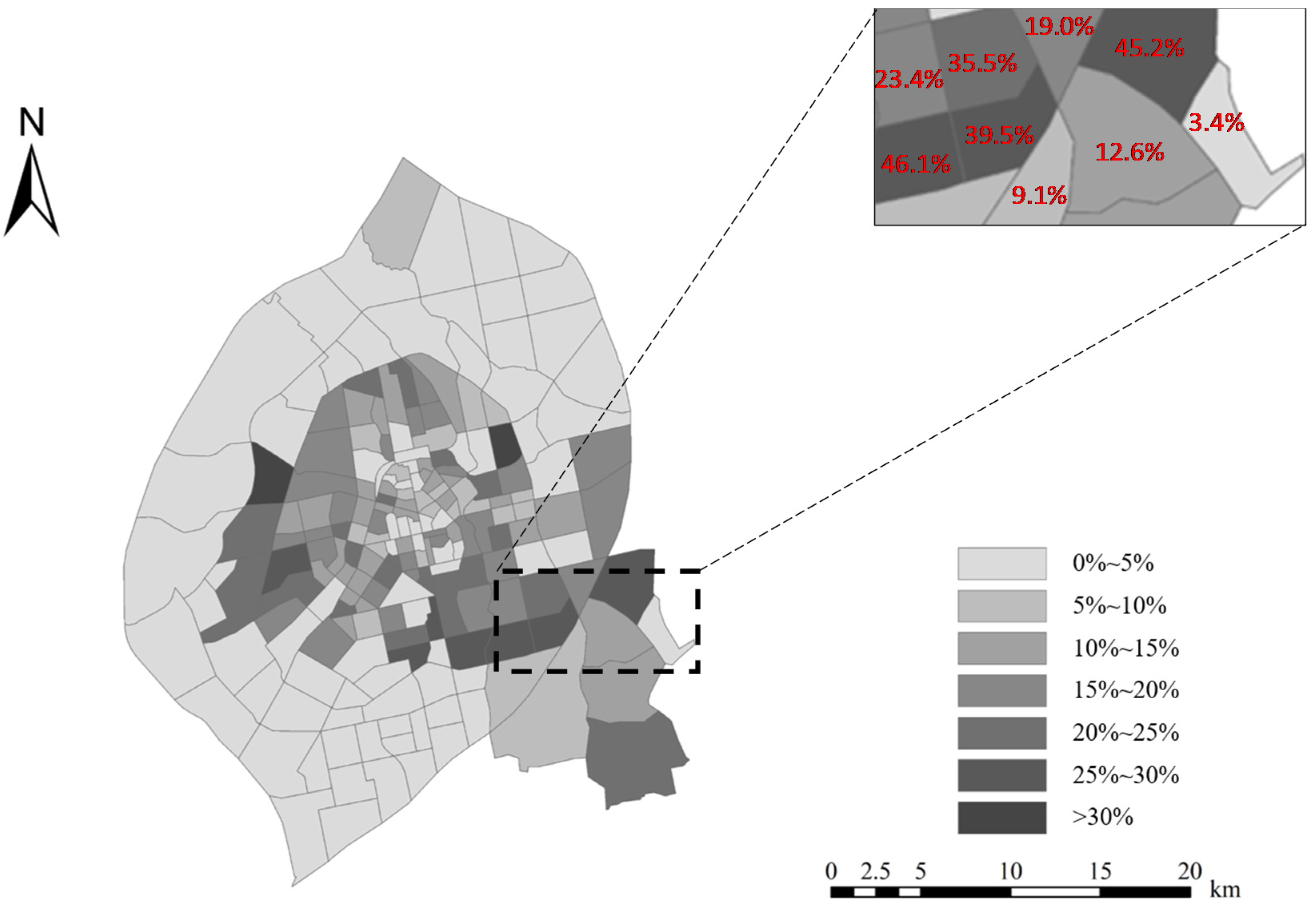
The primary data comes from the 2012 Changchun household travel survey, which was conducted by the Beijing Transport Institute and Changchun Institute of Urban Planning and Design from 1 May 2012 to 13 May 2012. The survey is the most recent travel survey in Changchun, which is representative of the city. The survey region includes Nanguan District, Chaoyang District, Kuancheng District, Erdao District, and Lvyuan District. The total samples include 51,909 members from 20,000 households. The sampling rate is 0.68%. In addition, 3,651 households have one or more cars, which take up 18.2% of the total samples. The proportion of households that own at least one car in the traffic analysis zones (TAZs) is shown in Figure 2. The travel survey data includes all the complete travel information on an assigned workday of the respondents. After error checking, we randomly selected one member’s commuting trip data from each household. Finally, 12,977 commuting trips were used for this study.

The socio-economic characteristics include individual characteristics and household characteristics in this study. The individual characteristics include the respondent’s gender, age, and education level. The household characteristics include the Hukou type, household size, household income, car ownership status, and the willingness to purchase a car for the households without cars. The descriptive statistics of socio-economic characteristics are shown in

Table 1. Variables and descriptions used for analysis.

Variables	Variable Description	Case/Mean	Percentage/Std. Dev.
Individual characteristics
Gender	=0 if the gender of the respondent is female	6684	58.27
	=1 if the gender of the respondent is male
Age	=1 if the age of the respondent is between 0-24; otherwise = 0	1059	9.23
	=2 if the age of the respondent is between 25-34; otherwise = 0	3780	32.95
	=3 if the age of the respondent is between 35-44; otherwise = 0	3872	33.75
	=4 if the age of the respondent is more than 45; otherwise = 0	2763	24.09
Education level	= 1 if respondent completed college degree; otherwise = 0	4060	35.40
Hukou	=1 if respondent has local Hukou; otherwise = 0	10,828	94.39
Household characteristics
Household size	=1 if number of members in household is 1; otherwise = 0	213	1.86
	=2 if number of members in household is 2; otherwise = 0	2662	23.21
	=3 if number of members in household is 3; otherwise = 0	6623	57.74
	=4 if number of members in household is 4; otherwise = 0	1199	10.45
	=5 if the age of the respondent is more than 5; otherwise = 0	778	6.78
Household students	Number of students in household	1.22	0.83
Household workers	Number of workers in household	2.31	1.89
Household income 1	=1 if household yearly income is less than 20000 RMB ; otherwise = 0	371	3.23
Household income 2	=1 if household yearly income is more than 100000 RMB ; otherwise = 0	1527	13.31
Car ownership	=1 if household own one or more cars; otherwise = 0	2775	24.19
Without car and has no propensity of purchasing one in two years	=1 if response has no cars in their household at present and has no intention of purchasing one in two years; otherwise = 0	10,636	92.72
Without car but has the intention of purchasing one in two years	=1 if response has no cars in their household at present but has the intention of purchasing one in two years; otherwise = 0	834	7.27
Travel-related characteristics
Travel mode	=1 if response commutes by car; otherwise = 0	1844	16.08
Commuting distance(km)	Distance traveled by commuter from home to workplace	5.625	10.266
Built environment characteristics
Home-Land use mixture	Land use mixture in residential areas	0.593	0.068
Home-Transit station density	Transit station density in residential areas	10.485	5.940
Home-Intersection density	Intersection density in residential areas	33.346	34.697
Home-Distance to CBD	Distance to CBD (home)	9.642	6.024
Workplace-Land use mixture	Land use mixture in employment areas	0.598	0.072
Workplace-Transit station density	Transit station density in employment areas	8.771	6.094
Workplace-Intersection density	Intersection density in employment areas	26.627	32.131
Workplace-Distance to CBD	Distance to CBD (workplace)	8.698	5.779
Parking availability
Home-parking density	Parking density in residential areas	93.170	83.840
Workplace- parking density	Parking density in employment areas	72.210	81.041
Home-close to a parking (500 m buffer)	=1 if there are parking spaces close to the residence within 500 m buffer; otherwise = 0	3133	27.31
Workplace- close to a parking (500 m buffer)	=1 if there are parking spaces close to the workplace within 500 m buffer; otherwise = 0	4955	43.20

. The socio-economic characteristics can reflect the people’s living conditions in Changchun due to the fact that the 2012 Changchun household travel survey is the most recent travel survey, which is representative of the Changchun city.

Urban built environment consists of land use, urban design, and traffic system. To explore the influence of the built environment on car ownership and use, four types of variables are used to measure the built environment in this study. They are design (intersection density), distance to transit (transit station density), destination (distance to Central Business District (CBD)), and diversity (land use mixture). The built environment variables are defined and described as follows.

Intersection density: intersection number per square kilometer at TAZ level. Intersection density represents the road network characteristics in the TAZs. This variable was obtained using ArcGIS software and it was calibrated based on the Changchun Traffic Map.

Transit station density: transit station number per square kilometer at TAZ level. Transit station density is used to measure the transit accessibility. Transit stations include bus stops and metro stations. Transit station density was calibrated based on the points of interest (POIs) extracted from AMAP, which is one of the most popular web mapping service applications in China.

Distance to CBD: distance to CBD in kilometers. Distance to CBD represents the spatial location of the residence or workplace. We extracted the centroid point coordinates of TAZs and calibrated the shortest distance along road links between centroid point coordinates of TAZs and CBD.

Land use mixture: measurement of degree of different types of land use composition. Land use mixture is used to measure the diversity of land use. Due to the lack of land use data, we used AMAP Application Programming Interface (API) to extract POIs including residence, hotel, restaurant, supermarket, park, square, mall, school, hospital, bank, and government. An entropy method was used to calibrate the land use mixture based on the POIs, following Wang et al. [22]. The entropy value can be calibrated as follows:

$$E_j=\frac{-{\displaystyle \sum p_{ij}\ln p_{ij}}}{\ln N_j}$$

(1)

where $p_{ij}$ is the proportion of POI type $i$ found in TAZ $j$, and $N_j$ is the total number of all POIs in TAZ $j$. $E_j$ is the entropy value of TAZ $j$. The value ranges from 0 to 1 and higher value represents a more balanced land use mixture.

Parking availability is used to measure the parking accessibility around residences and workplaces. The parking availability around the residence and workplace is measured by two indexes, respectively. The first index is the parking density in the TAZs. The second one is whether there are parking lots within the 500 m buffer around the residence and workplace or not. We used AMAP Application Programming Interface (API) to extract POIs and ArcGIS software to calibrate the parking density. The parking availability within 500 m buffer was obtained using ArcGIS software.

The travel-related characteristics include commuting mode and commuting distance. Commuting mode was defined as a binary variable according to whether the respondent goes to work by car or not. The commuting distance was calibrated using the shortest path based on the origin and end of the trip.

3.3. Method

There were four models in this study. The binary logistic model was employed to explore the determinants of car ownership and use. The dependent variables were car ownership status for all households and the intention of purchasing a car in two years for the households without cars in the former two models, respectively. First, we analyzed how built environment and parking availability influenced whether the household owned cars and planned to purchase one in two years or not. The first model was used to explore the determinants of car ownership for all households. Car ownership status of the household was defined as a binary variable. The second model aimed to explore the determinants of the intention of purchasing a car in two years for the households without cars. Then, we analyzed how built environment and parking availability both at the start and at the end of the trip influenced car use for commuting in the latter models. In order to investigate the influence of parking availability on car use, two logistic models were employed. The third model only revealed the influence of built environment and socio-economic characteristics on car use for the journey to work as comparison, whereas parking availability was considered in the final model.

Binary logistic models are usually used to predict the probability of occurrence for some binary explained variables according to the explanatory variables. In this study, the explained variables included car ownership status for all households, intention of purchasing a car for the households without cars, and car use for commuting, respectively. The explained variable is set to be one when it occurs. Otherwise, it is set as zero. The explanatory variables include social-economic characteristics, built environment characteristics, and parking availability. Then the binary logistic model is represented as follows:

$$P(Y=1)=\frac{1}{1+\exp [-({\beta }_0+{\beta }_1{X}_1+{\beta }_2{X}_2+\cdots +{\beta }_k{X}_k)]}$$

(2)

where $Y$ is the the explained variable; ${\beta }_0$, ${\beta }_1$, ${\beta }_2\cdots {\beta }_k$ are the estimated parameters of explanatory variables; $X_1$, $X_2\cdots X_k$ are the explanatory variables.

In this study, the four binary logistic models are calibrated according to the maximum likelihood estimation method. All the estimations and computations are carried out by using SPSS software, version 24.

4. Results and Discussion

4.1. Determinants of Car Ownership

Table 2. Binary logistic regression of household car ownership.

Variables	Model 1: All Samples			Model 2: For Households without Cars Only
Independent Variable	Coefficient	Sig.	Exp(B)	Coefficient	Sig.	Exp(B)
Household characteristics
Household size	0.037		1.038	0.194	**	1.214
Household income 1	−0.055	**	0.946	−0.377	*	0.686
Household income 3	0.032	**	1.033	0.072	**	1.075
Household students	0.087	**	1.091	0.248	**	1.281
Household workers	0.013		1.013	0.037	*	1.038
Travel-related characteristics
Commuting distance	0.026	**	1.026	0.028		1.028
Built environment characteristics
Home-Land use mixture	1.193	**	3.297	1.510	**	4.527
Home-Transit station density	−0.019	**	0.981	−0.004	*	0.996
Home-Intersection density	−0.007	**	0.993	−0.003		0.997
Home-Distance to CBD	0.178	**	1.195	−0.023		0.977
Workplace-Land use mixture	0.667	*	1.948	−0.416		0.660
Workplace-Transit station density	−0.003		0.997	0.004		1.004
Workplace-Intersection density	−0.006		0.994	−0.013	*	0.987
Workplace-Distance to CBD	0.047	**	1.048	−0.052		0.949
Parking availability
Home-parking density	0.011	**	1.011	0.009	*	1.009
Workplace- parking density	0.005	**	1.005	0.002		1.002
Home-close to a parking (500 m buffer)	0.021	**	1.021	0.006	*	1.006
Workplace- close to a parking (500 m buffer)	0.027	**	1.027	0.022		1.022
Constant	−4.334	**	0.013	−3.287	**	0.037
R2	0.632			0.546

Note: ** and * denote significance at the levels of 95% and 90%, respectively.

presents the results of car ownership and intention of purchasing a car in two years for households without cars. After controlling for the other variables, some built environment variables still have significant influence on car ownership and the intention of purchasing a car. The coefficients of transit station density and intersection density in residential areas are −0.019 and −0.007, respectively. The results show that transit station density and intersection density in residential areas have significantly negative relations with car ownership at the significance level of 95%. This means that households living in areas with higher transit station density and intersection density have a lower probability of owning cars. According to the results, distance to CBD from residence shows a significantly positive (0.178) relation with car ownership at the significance level of 95%. It indicates that households living far from CBD are more likely to own a car. Additionally, the results indicate that land use mixture is also a factor that can influence household car ownership status. As the land use mixture increases, the odd of owning cars becomes higher. The influence of land use mixture in residential areas is consistent with some existing studies [11,54]. This might be explained by the fact that people living in compact land use areas encounter shorter distances, thus cutting down the travel cost and further reducing the cost of car ownership. Moreover, land use mixture and transit station density in residential areas are also significantly associated with car ownership propensity for households without cars at the significance level of 95% and 90% respectively (1.510 for land use mixture and −0.004 for transit station density). Households living in the areas with lower transit station density and compact land use mixture have a stronger propensity of owning cars in two years. For the workplace built environment, land use mixture and distance to CBD have significantly positive influences on car ownership, which is similar with the influence of residential built environment. In addition, only the intersection density at job location is found to be significantly related with the car ownership propensity.

As shown in Table 2, parking availability variables play a remarkable role in determining car ownership. It is found that the effect of parking proximity within 500 m buffer and parking density in residential areas on car ownership and intentions of purchasing a car in two years is significantly positive. It means that parking convenience raises the probability of car ownership and intentions of purchasing a car. This might be explained by the fact that residential parking availability plays an important role in making the car purchasing decision. The coefficients of parking proximity within the 500 m buffer and parking density in workplace areas are 0.027 and 0.005. The results show that they are only significantly associated with car ownership at the significance level of 95%. However, the influence on car ownership intention is not significant. This may be because, when residents make car ownership purchase decision, parking availability in residential areas and other driving demands for non-work purposes are also important.

Most household characteristics and travel-related characteristics show significant influence on car ownership and the intention of purchasing a car. The coefficients of household income in model 1 are −0.055 and 0.032. And the coefficients in model 2 are −0.377 and 0.072, respectively. The results show that household income is significantly related with car ownership and the intentions of purchasing a car. These results indicate that households with higher income have a higher probability of owning cars and stronger will to purchase a car in the future. The result is consistent with most previous studies because household income restrains the cost of purchasing and use [40,42,54]. The number of household students is both related with household car ownership and purchase intention. Additionally, household workers are only related with the purchase intention. Household size is not associated with car ownership. However, it is shown that bigger households tend to own cars in two years. Commuting distance is another factor that only influences car ownership.

4.2. Determinants of Car Use

Table 3. Binary logistic regression of car use.

	Model 3: Car Use Model Ignoring Parking Availability			Model 4: Car Use Model Considering Parking Availability
Independent Variable	Coefficient	Sig.	Exp(B)	Coefficient	Sig.	Exp(B)
Individual characteristics
Gender	1.994	**	7.345	1.987	**	7.294
Age	0.112	*	1.119	0.111	*	1.117
Education level	0.877	**	2.404	0.867	**	2.380
Hukou	0.131	*	1.140	0.119	*	1.126
Household characteristics
Household size	0.058		1.060	0.063		1.065
Household income 1	−0.015	*	0.985	-0.012	*	0.988
Household income 3	0.068	*	1.070	0.067	*	1.069
Household students	0.024		1.024	0.026		1.026
Household workers	0.157	**	1.170	0.142	**	1.153
Car ownership	1.487	**	4.424	1.538	**	4.655
Travel-related characteristics
Commuting distance	0.026	**	1.026	0.026	**	1.026
Built environment characteristics
Home-Land use mixture	−1.214	*	0.297	−1.225	*	0.294
Home-Transit station density	−0.012	*	0.988	−0.011	**	0.989
Home-Intersection density	−0.001		0.999	0.000		1.000
Home-Distance to CBD	0.137	**	1.147	0.112	**	1.119
Workplace-Land use mixture	0.625		1.868	−0.543	**	0.581
Workplace-Transit station density	−0.008	*	0.992	−0.006	*	0.994
Workplace-Intersection density	0.003		1.003	−0.002	*	0.998
Workplace-Distance to CBD	0.026	*	1.026	0.013	*	1.013
Parking availability
Home-parking density	—	—	—	0.019	**	1.019
Workplace-parking density	—	—	—	0.006	**	1.006
Home-close to a parking (500 m buffer)	—	—	—	0.023	**	1.023
Workplace-close to a parking (500 m buffer)	—	—	—	0.012	**	1.012
Constant	−9.635	**	0.000	−9.428	**	0.000
R2	0.768			0.876

Note: ** and * denote significance at the levels of 95% and 90%, respectively.

presents the regression results of car use. In this study, Nagelkerke R² is used to assess the model fit. Generally, a higher value of Nagelkerke R² identifies a better fitting model. When comparing the model fit information between these two models, the final model considering parking availability fit better. The result indicates that parking availability cannot be ignored when exploring the influence of socio-economic characteristics and built environment on car dependency.

The results of the third model show that built environment can influence the respondents’ commuting mode choice after controlling for socio-economic characteristics and travel-related information. It is found that residential land use mixture has significantly negative (−1.214) association with car use for the journey to work at the significance level of 90%, which is consistent with existing studies [12]. Moreover, residents living in areas with higher transit station density have a lower probability of commuting by car. Distance to CBD is also a factor that can influence the commute mode choice significantly. People living farther from the CBD commute by car more. It might be explained by the fact that most employment opportunities concentrate around the CBD, which increases the commuting distance of residents living in suburban districts. Residential intersection density has no significant influence on commuting mode choice. The influence of workplace built environment is similar with that of the residence. The results show that land use mixture has few influences on commuting mode choice. Additionally, the coefficient (0.026) of distance to CBD is significant and positive at the significance level of 90%, suggesting that a workplace which is farther from the CBD can increase the probability of commuting by car. As transit station density increases, residents have a lower probability of commuting by car (Coeff. = −0.008). Moreover, workplace intersection density is not related with commuting mode choice.

Similar to car ownership, most socio-economic characteristics and travel-related information have significant influences on commuting mode choice. Men are found to be more likely to commute by car. In addition, age has a significantly positive influence on commuting by car at the significance level of 90% (Coeff. = 0.112). The coefficient of education level is 0.877. The results suggest that people who have completed college degrees have a higher probability of commuting by car than others. Hukou system is a special system conducted in China to prevent population mobility and it also has a positive influence on car use for commuting at the significance level of 90% (Coeff. = 0.131). This means that people with local Hukou generate more car commuting trips. Household income is also positively associated with commuting by car. Additionally, household students are not associated with car commuting. Commuters living in households with more workers have a higher probability of commuting by car (Coeff. = 0.157). Moreover, residents from the households owning cars tend to commute by car more than others. It is found that household size has no significant influence on commuting mode choice. What’s more, commuting distance is positively associated with the probability of car commuting, which is consistent with the previous study [23].

Parking availability is used to measure the parking convenience, which can produce influence on commuting mode choice [17,35]. Therefore, it can lead to mis-estimating the influence of built environment on car commuting when ignoring the influence of parking availability. After incorporating the parking availability into the third model, the model fits the data better, as shown in Table 3. Most of the influences do not show substantial changes, except for the workplace intersection density and land use mixture, which become significant in model 4. However, the power of other factors has changed. As shown in Table 3, the results show that the parking availability variables at residence and workplace are all significant (0.019 and 0.023 for residence, 0.006 and 0.012 for workplace) at the significance level of 95%. These results demonstrate the effect of parking availability, which should not be ignored in the model. After controlling for the socio-economic characteristics and built environment characteristics, parking density at residence and workplace is positively associated with car use for the journey to work. Moreover, parking proximity at residences and workplaces can encourage car use to some extent. After controlling for socio-economic characteristics and parking availability, except for the residential land use mixture, the influence of other built environment characteristics decreases. Therefore, the third model mis-estimates the influence of the built environment due to the lack of parking availability variables.

5. Conclusion and Policy Implications

This study explored the joint effect of the built environment and parking availability on car ownership and use under a rapidly urbanizing and motorizing context of Changchun, China. The binary logistic model was used to investigate the effects. Results show that after controlling for the socio-economic characteristics and parking availability, built environment is still significantly associated with car ownership and use, which confirmed the existing studies [55,56,57,58]. Moreover, the results demonstrate the effect of parking availability, which cannot be ignored when exploring the influence of built environment on car ownership and use. Specifically, car ownership is significantly associated with parking availability in residence and workplace neighborhood, most built environment characteristics except for the transit station density and intersection density in workplace neighborhood, household income, household students and commuting distance. In addition, bigger household size, higher household income, more household students, more household workers, compact land use mixture, and lower transit station density in residence neighborhood, lower intersection density in workplace neighborhood, better parking availability and parking proximity can increase the odds of purchasing a car for households without cars. Regarding car use decisions, all factors, including socio-economic characteristics, built environment characteristics, and parking availability, in this study, show significant association with car use for commuting except for household size, household students and intersection density in residential areas.

The findings of this study have some policy implications, which could help develop efficient policies to reduce car ownership and use, thus saving energy and reducing pollutant emissions further. First, it is desirable for urban planners and policy makers to develop strategies to reduce car dependency for small and mid-sized cities like Changchun. The results reveal that a wide range of built environment characteristics from residence to job location can influence car dependency. While the residential built environment characteristics are more influential on commute behavior than the characteristics at job location, built environment at job location should not be ignored. Second, parking supply is a key factor that could have influence on car dependency. The results suggest that parking restrictions at both residence and workplace could reduce the odds of using a car for the journey to work. Therefore, it would be wise for urban planners to moderately restrict the parking supply and increase the distance between parking and workplace. Third, results show that higher transit station density can help produce important positive outcomes, which strongly suggests that transit-oriented development (TOD) is an effective strategic approach for urban expansion. Therefore, urban planners and policy makers should facilitate a strategic approach in China. Finally, Hukou is a special system conducted to control population mobility and the socio-welfare distribution in China, which is rather different from western cities. The results indicate that commuting trips with local Hukou increase the likelihood of driving to work. Therefore, policy makers should pay more attention to these groups of people and promote quota control policies for car ownership and use.

One limitation of this study should be noted in future work. Parking availability is only captured using the parking density and parking proximity at residence and workplace due to the lack of other variables. To solve this problem, more related variables, such as parking fees, should be considered for follow-up work.

References

- Mu, R.; de Jong, M. A Tale of Two Chinese Transit Metropolises and the Implementation of Their Policies: Shenyang and Dalian (Liaoning Province, China). Energies 2018, 11, 18. [Google Scholar] [CrossRef]
- National Bureau of Statistics. China Statistic Yearbook 2013; China Statistics Press: Beijing, China, 2013. [Google Scholar]
- Li, S.; Zhao, P. Exploring car ownership and car use in neighborhoods near metro stations in Beijing: Does the neighborhood built environment matter? Transp. Res. Part D 2017, 56, 1–17. [Google Scholar] [CrossRef]
- Zhang, R.; Yao, E.; Liu, Z. School travel mode choice in Beijing, China. J. Transp. Geogr. 2017, 62, 98–110. [Google Scholar] [CrossRef]
- Cao, X.; Huang, X. City-level determinants of private car ownership in China. Asian Geogr. 2013, 30, 37–53. [Google Scholar] [CrossRef]
- Chen, X.; Zhang, H. Evaluation of Effects of Car Ownership Policies in Chinese Megacities. Transp. Res. Rec. J. Transp. Res. Board 2012, 2317, 32–39. [Google Scholar] [CrossRef]
- Badland, H.M.; Garrett, N.; Schofield, G.M. How Does Car Parking Availability and Public Transport Accessibility Influence Work-Related Travel Behaviors? Sustainability 2010, 2, 576–590. [Google Scholar] [CrossRef]
- Guo, Z. Home parking convenience, household car usage, and implications to residential parking policies. Transp. Policy 2013, 29, 97–106. [Google Scholar] [CrossRef]
- Guo, Z. Does residential parking supply affect household car ownership? The case of New York City. Transp. Geogr. 2013, 26, 18–28. [Google Scholar] [CrossRef]
- Ding, C.; Lin, Y.; Liu, C. Exploring the influence of built environment on tour-based commuter mode choice: A cross-classified multilevel modeling approach. Transp. Res. Part D 2014, 32, 230–238. [Google Scholar] [CrossRef]
- Ding, C.; Liu, C.; Zhang, Y.; Yang, J.; Wang, Y. Investigating the impacts of built environment on vehicle miles traveled and energy consumption: Differences between commuting and non-commuting trips. Cities 2017, 68, 25–36. [Google Scholar] [CrossRef]
- Ding, C.; Wang, D.; Liu, C.; Zhang, Y.; Yang, J. Exploring the influence of built environment on travel mode choice considering the mediating effects of car ownership and travel distance. Transp. Res. Part A 2017, 100, 65–80. [Google Scholar] [CrossRef]
- Cervero, R. Built environments and mode choice: Toward a normative framework. Transp. Res. Part D 2002, 7, 265–284. [Google Scholar] [CrossRef]
- Cervero, R.; Lsarmiento, O.; Jacoby, E.; Gomez, L.F.; Nei-Man, A.; Xue, G. Influences of Built Environments on Walking and Cycling: Lessons from Bogotá. Urban Transp. China 2016, 3, 203–226. [Google Scholar] [CrossRef]
- Cervero, R. The built environment and travel: Evidence from the United States. Eur. J. Transp. Infrastruct. Res. 2003, 3, 119–137. [Google Scholar]
- Jiang, Y.; Gu, P.; Chen, Y.; He, D.; Mao, Q. Influence of land use and street characteristics on car ownership and use: Evidence from Jinan, China. Transp. Res. Part D 2017, 52, 518–534. [Google Scholar] [CrossRef]
- Christiansen, P.; Engebretsen, Ø.; Fearnley, N.; Hanssen, J.U. Parking facilities and the built environment: Impacts on travel behaviour. Transp. Res. Part A 2017, 95, 198–206. [Google Scholar] [CrossRef]
- Sun, B.; Ermagun, A.; Dan, B. Built environmental impacts on commuting mode choice and distance: Evidence from Shanghai. Transp. Res. Part D 2017, 52, 441–453. [Google Scholar] [CrossRef]
- Naess, P. Urban form and travel behavior: Experience from a Nordic context. J. Transp. Land Use 2012, 5, 21–45. [Google Scholar] [CrossRef]
- Naess, P. ‘New urbanism’ or metropolitan-level centralization? A comparison of the influences of metropolitan-level and neighborhood-level urban form characteristics on travel behavior. J. Transp. Land Use 2011, 4, 25–44. [Google Scholar] [CrossRef]
- Ding, C.; Wang, Y.; Tang, T.; Mishra, S.; Liu, C. Joint analysis of the spatial impacts of built environment on car ownership and travel mode choice. Transp. Res. Part D 2018, 60, 28–40. [Google Scholar] [CrossRef]
- Ewing, R.; Cervero, R. Travel and the Built Environment: A Meta-Analysis. J. Am. Plan. Assoc. 2001, 76, 265–294. [Google Scholar] [CrossRef]
- Wang, X.; Shao, C.; Yin, C.; Zhuge, C.; Li, W. Application of Bayesian Multilevel Models Using Small and Medium Size City in China: The Case of Changchun. Sustainability 2018, 10, 484. [Google Scholar] [CrossRef]
- Zegras, C. The Built Environment and Motor Vehicle Ownership and Use: Evidence from Santiago de Chile. Urban Stud. 2010, 47, 1793–1817. [Google Scholar] [CrossRef]
- Acker, V.V.; Witlox, F. Car ownership as a mediating variable in car travel behaviour research using a structural equation modelling approach to identify its dual relationship. J. Transp. Geogr. 2010, 18, 65–74. [Google Scholar] [CrossRef] [Green Version]
- Wu, W.; Hong, J. Does public transit improvement affect commuting behavior in Beijing, China? A spatial multilevel approach. Transp. Res. Part D 2016, 52, 471–479. [Google Scholar] [CrossRef]
- Ding, C.; Mishra, S.; Lu, G.; Yang, J.; Liu, C. Influences of built environment characteristics and individual factors on commuting distance: A multilevel mixture hazard modeling approach. Transp. Res. Part D 2017, 51, 314–325. [Google Scholar] [CrossRef]
- Hong, J.; Chen, C. The role of the built environment on perceived safety from crime and walking: Examining direct and indirect impacts. Transportation 2014, 41, 1171–1185. [Google Scholar] [CrossRef]
- Zhang, L.; Hong, J.H.; Nasri, A.; Shen, Q. How Built Environment Affects Travel Behavior: A Comparative Analysis of the Connections between Land Use and Vehicle Miles Traveled in U.S. Cities. J. Transp. Land Use 2012, 5, 40–52. [Google Scholar] [CrossRef]
- Wheeler, S.M.; Tomuta, M.; Haden, V.R.; Jackson, L.E. The impacts of alternative patterns of urbanization on greenhouse gas emissions in an agricultural county. J. Urban Int. Res. Placemaking Urban Sustain. 2013, 6, 213–235. [Google Scholar] [CrossRef]
- Hamre, A.; Buehler, R. Commuter Mode Choice and Free Car Parking, Public Transportation Benefits, Showers/Lockers, and Bike Parking at Work: Evidence from the Washington, DC Region. J. Public Trans. 2014, 17, 67–91. [Google Scholar] [CrossRef] [Green Version]
- Su, Q.; Zhou, L. Parking management, financial subsidies to alternatives to drive alone and commute mode choices in Seattle. Reg. Sci. Urban Econ. 2012, 42, 88–97. [Google Scholar] [CrossRef]
- Albert, G.; Mahalel, D. Congestion tolls and parking fees: A comparison of the potential effect on travel behavior. Transp. Policy 2008, 13, 496–502. [Google Scholar] [CrossRef]
- Willson, R.W.; Shoup, D.C. Parking subsidies and travel choices: Assessing the evidence. Transportation 1990, 17, 141–157. [Google Scholar] [CrossRef] [Green Version]
- Liu, Q.; Wang, J.; Chen, P.; Xiao, Z. How does parking interplay with the built environment and affect automobile commuting in high-density cities? A case study in China. Urban Stud. 2017, 54, 3299–3317. [Google Scholar] [CrossRef]
- Rye, T.; Cowan, T.; Ison, S. Expansion of a Controlled Parking Zone (CPZ) and its Influence on Modal Split: The Case of Edinburgh. Transp. Plan. Tech. 2006, 29, 75–89. [Google Scholar] [CrossRef]
- Weinberger, R. Death by a thousand curb-cuts: Evidence on the effect of minimum parking requirements on the choice to drive. Transp. Policy 2012, 20, 93–102. [Google Scholar] [CrossRef]
- Kitamura, R.; Akiyama, T.; Yamamoto, T.; Golob, T.F. Accessibility in a Metropolis: Toward a Better Understanding of Land Use and Travel. Transp. Res. Rec. J. Transp. Res. Board 2001, 1780, 64–75. [Google Scholar] [CrossRef]
- Mokhtarian, P.L.; Cao, X.; Handy, S.L. Cross-sectional and quasi-panel explorations of the connection between the built environment and auto ownership. Environ. Plan. A Econ. Space 2007, 39, 830–847. [Google Scholar] [CrossRef]
- Giuliano, G.; Dargay, J. Car ownership, travel and land use: A comparison of the US and Great Britain. Transp. Res. Part A 2006, 40, 106–124. [Google Scholar] [CrossRef]
- Cao, X.; Yang, W. Examining the effects of the built environment and residential self-selection on commuting trips and the related CO2 emissions: An empirical study in Guangzhou, China. Transp. Res. Part D 2017, 52, 480–494. [Google Scholar] [CrossRef]
- Paulley, N.; Balcombe, R.; Mackett, R.; Titheridge, H.; Preston, J.; Wardman, M.; Shires, J.; White, P. The demand for public transport: The effects of fares, quality of service, income and car ownership. Transp. Policy 2006, 13, 295–306. [Google Scholar] [CrossRef] [Green Version]
- Jong, G.D.; Fox, J.; Daly, A.; Pieters, M.; Smit, R. Comparison of car ownership models. Transp. Rev. 2004, 24, 379–408. [Google Scholar] [CrossRef] [Green Version]
- Jiang, Y.; Zhang, J.; Jin, X.; Ando, R.; Chen, L.; Shen, Z.; Ying, J.; Fang, Q.; Sun, Z. Rural migrant workers’ intentions to permanently reside in cities and future energy consumption preference in the changing context of urban China. Transp. Res. Part D 2017, 52, 600–618. [Google Scholar] [CrossRef]
- Hong, J.; Shen, Q. Residential density and transportation emissions: Examining the connection by addressing spatial autocorrelation and self-selection. Transp. Res. Part D 2013, 22, 75–79. [Google Scholar] [CrossRef]
- Aditjandra, P.T.; Cao, X.; Mulley, C. Understanding neighbourhood design impact on travel behaviour: An application of structural equations model to a British metropolitan data. Transp. Res. Part A 2012, 46, 22–32. [Google Scholar] [CrossRef]
- Cao, J.; Ettema, D.; Levinson, D.M. Satisfaction with travel and residential self-selection: How do preferences moderate the impact of the Hiawatha Light Rail Transit line? J. Transp. Land Use 2014, 7, 93–108. [Google Scholar] [CrossRef]
- Cao, J.; Cao, X. The impacts of LRT, neighbourhood characteristics, and self-selection on auto ownership: Evidence from Minneapolis-St. Paul. Urban Stud. 2014, 51, 2068–2087. [Google Scholar] [CrossRef]
- Zhao, P.; Li, S. Bicycle-metro integration in a growing city: The determinants of cycling as a transfer mode in metro station areas in Beijing. Transp. Res. Part A 2017, 99, 46–60. [Google Scholar] [CrossRef]
- Hong, J.; Shen, Q.; Zhang, L. How do built-environment factors affect travel behavior? A spatial analysis at different geographic scales. Transportation 2014, 41, 419–440. [Google Scholar] [CrossRef]
- Ding, C.; Chen, Y.; Duan, J.; Lu, Y.; Cui, J. Exploring the Influence of Attitudes to Walking and Cycling on Commute Mode Choice Using a Hybrid Choice Model. J. Adv. Transp. 2017, 2017, 1–8. [Google Scholar] [CrossRef]
- Ministry of Transport Information Disclosure. Notice of the Ministry of Transport on Promulgating the Second Batch of Cities for Demonstration Construction of Transit Metropolis. Available online: http://zizhan.mot.gov.cn/zfxxgk/bnssj/dlyss/201311/t20131122_1516513.html (accessed on 21 November 2013).
- National Bureau of Statistics. China Statistic Yearbook 2014; China Statistics Press: Beijing, China, 2014. [Google Scholar]
- Hess, D.B.; Ong, P.M. Traditional Neighborhoods and Auto Ownership. Transp. Res. Rec. J. Transp. Res. Board 2001, 1805. [Google Scholar] [CrossRef]
- Dargay, J.; Gately, D. Income’s effect on car and vehicle ownership, worldwide: 1960–2015. Transp. Res. Part A 1999, 33, 101–138. [Google Scholar] [CrossRef]
- Zhao, P. The Impact of the Built Environment on Individual Workers’ Commuting Behavior in Beijing. Int. J. Sustain. Transp. 2013, 7, 389–415. [Google Scholar] [CrossRef]
- Zhang, Y.; Wu, W.; Li, Y.; Liu, Q.; Li, C. Does the Built Environment Make a Difference? An Investigation of Household Vehicle Use in Zhongshan Metropolitan Area, China. Sustainability 2014, 6, 4910–4930. [Google Scholar] [CrossRef] [Green Version]
- Susilo, Y.O.; Maat, K. The influence of built environment to the trends in commuting journeys in the Netherlands. Transportation 2007, 34, 589–609. [Google Scholar] [CrossRef] [Green Version]
Figure 1.
Study area and parking facilities distribution.
Figure 2.
The proportion of car ownership households in the traffic analysis zones (TAZs).