Agroecological Pest Management in the City: Experiences from California and Chiapas
by
 , ,
, ,
Helda Morales
1, 
Bruce G. Ferguson
1,
Linda E. Marín
1,
Dario Navarrete Gutiérrez
2,
Peter Bichier
3 and
Stacy M. Philpott
3,* 1
Departamento de Agricultura, Sociedad y Ambiente, El Colegio de la Frontera Sur, San Cristóbal de Las Casas, Chiapas 29290, Mexico
2
Laboratorio de Análisis de Información Geográfica y Estadística, El Colegio de la Frontera Sur, San Cristóbal de Las Casas, Chiapas 29290, Mexico
3
Environmental Studies Department, University of California, Santa Cruz, Santa Cruz, CA 95064, USA
*
Author to whom correspondence should be addressed.
Sustainability 2018, 10(6), 2068; https://doi.org/10.3390/su10062068
Submission received: 24 April 2018
/
Revised: 8 June 2018
/
Accepted: 12 June 2018
/
Published: 19 June 2018
(This article belongs to the Special Issue Agroecology in the City: Applying Ecological Principles to Sustainable Urban Agriculture)
Abstract
:Urban gardens are a prominent part of agricultural systems, providing food security and access within cities; however, we still lack sufficient knowledge and general principles about how to manage pests in urban agroecosystems in distinct regions. We surveyed natural enemies (ladybeetles and parasitoids) and conducted sentinel pest removal experiments to explore local management factors and landscape characteristics that influence the provisioning of pest control services in California, USA, and Chiapas, Mexico. We worked in 29 gardens across the two locations. In each location, we collected data on garden vegetation, floral availability, ground cover management, and the percentage of natural, urban, and agricultural land cover in the surrounding landscape. We sampled ladybeetles, Chalcidoidea, and Ichneumonoidea parasitoids with sticky traps, and monitored the removal of three different pest species. Ladybeetle abundance did not differ between locations; abundance decreased with garden size and with tree cover and increased with herbaceous richness, floral abundance, and barren land cover. Chalcicoidea and Ichneumonoidea parasitoids were more abundant in Chiapas. Chalcicoidea abundance decreased with herbaceous richness and with urban cover. Ichneumonoidea abundance increased with mulch and bare ground cover, garden size, garden age, and with agriculture land cover but decreased with tree richness and urban cover. Predators removed between 15–100% of sentinel prey within 24 h but prey removal was greater in California. Generally, prey removal increased with vegetation diversity, floral abundance, mulch cover, and urban land cover, but declined with vegetation cover and bare ground. Although some factors had consistent effects on natural enemies and pest control in the two locations, many did not; thus, we still need more comparative work to further develop our understanding of general principles governing conservation biological control in urban settings.
1. Introduction
Scientists, peasant organizations, and the UN Food and Agriculture Organization recognize that agroecology is essential to the production of healthy, culturally appropriate and abundant food [1,2]. Agroecological practices promote pest prevention in part by managing crop diversity and plot and landscape design to conserve and increase biological control agents [3,4]. Understanding the relationships underlying biological pest management is especially critical for urban gardens, given that the alternative—the use of chemical pesticides—may be especially damaging or risky for human populations living in close proximity. Urban farmers in the United States recognize that pests can be a problem in their gardens and that they do not have the knowledge to manage them [5]. However, urban gardens may serve as a refuge for a high diversity of biological control agents such as ladybeetles, parasitic wasps, carabids, spiders, ants and syrphid flies [6,7]. Populations of pests and natural enemies respond to site and landscape factors [8], but comparative work exploring how these relationships vary among geographic regions has been lacking. Such studies are essential to advance the development of general principles of urban ecology [9].
Although public and scientific interest in urban agriculture has grown dramatically in the past two decades, we still do not understand fully how to manage pests in a sustainable way in cities. An increasing number of studies have examined the roles of plant diversity, habitat area, landscape surroundings, and other local factors for urban garden beneficial insect biodiversity. For example, we now know that native plantings and floral abundance in urban gardens can benefit pest parasitoids [10]. Invertebrate diversity generally increases in gardens with high plant species diversity [11]. Some insects benefit from decreases in impervious cover in urban areas [12]. Nevertheless, the impact of garden characteristics and management on natural enemy communities may vary depending on the surrounding landscape and on arthropod life history [6,7,13,14,15].
Furthermore, only a few studies have documented biological control agents’ capacity to decrease pest populations [8,16,17]. In some areas, pest predation is high. Philpott and Bichier (2017) have documented 24-h predation rates between 40 and 90% in California, and Gardiner et al. (2009) reported more than 50% predation in 48 h in urban gardens in Ohio. Some of the factors identified as important for increasing pest predation and parasitism are vegetation complexity, garden size, ground cover features, and landscape diversity [8]. However, the influence of these factors may vary among groups of beneficial insects, among prey species, and among seasons [8,15].
As both urbanization and the popularity of urban gardening increase around the globe, understanding the impacts of garden management and landscape surroundings on biological control agents within gardens will become more important. Most, if not all, studies of urban biological control have been conducted in temperate areas. These studies identify important differences in biocontrol processes among study sites, and differences between tropical and temperate latitudes may be even greater.
With this in mind, we compare populations of natural enemies (predatory lady beetles and parasitoid wasps) and pest removal activity in urban gardens in the United States and Mexico, focusing specifically on California’s Central Coast and the Chiapas Highlands. We evaluate the influence of the landscape context and site factors that influence natural enemy populations and suggest management strategies that might enhance biological control services within these gardens.
2. Materials and Methods
2.1. Study Sites
We worked in two regions: the California central coast, USA and the Chiapas highlands, Mexico. The California central coast is an economically important region of the U.S. and is home to both Silicon Valley and what is often referred to as the nation’s ‘salad bowl’ [7]. Natural habitat in the area includes chaparral, grasslands, coastal sage scrub, oak woodlands, and coast redwood forests [18]. The climate is Mediterranean, with dry summers, wetter winters, and occasional frosts, with average annual rainfall between 380–800 mm per year [19]. San Cristobal, a city in the Chiapas highlands, is located in a valley at 2140 masl. The surrounding hillsides are mostly covered by pine-oak forest. Its climate is anti-Mediterranean, with wet summers and drier winters, occasional light frosts, and average annual rainfall of 1216 mm [20]. It is densely populated relative to the California cities. San Cristobal is among the oldest colonial cities in the Americas and its home garden traditions date to colonial times [21].
We worked in 18 urban community gardens in California in Santa Cruz, Monterey, and Santa Clara Counties and in 11 gardens (10 home gardens and one restaurant roof-top garden) in and around San Cristobal de Las Casas, Chiapas. Gardens in California were separated by between 2–90 km, and gardens in Chiapas were separated by between 0.5–7 km. Urban agriculture is highly variable and can appear in forms ranging from larger urban farms to small rooftop gardens [17]. In this study, the gardens selected varied in size (0.01–1.5 hectares) and in age (3–48 years old), but most gardens were small (<0.05 hectares). All gardens included vegetable patches that had been in regular cultivation for at least 3 years, and many also included various ornamental, native, and non-native plants. We included in our measure of garden size any cultivated area including vegetables, fruits, and ornamentals; the specific percentage of each garden dedicated to vegetable production varied, but we did not measure vegetable production area separately from fruits, orchards, or ornamentals in the same sites. All but one garden included direct cultivation in soil; the single roof top garden sampled was comprised of vegetables and flowers grown in raised beds and pots. In California, across all study gardens we recorded 58 crop species, and 88 other herbaceous plant species (ornamentals or weeds). In Chiapas, we recorded 40 crop species and 74 other herbaceous plant species (ornamentals or weeds). Common crops across both study regions included corn, beans, squash, tomatoes, tomatillos, and chard. All fieldwork in Chiapas was completed between 20–27 March 2015 and in California from 30 July–7 August 2015. The sampling periods correspond to the dry seasons of the respective regions.
Several previous studies have focused on understanding the impacts of local and landscape management of urban gardens on beneficial insects, such as ladybeetles, parasitoids, spiders, and bees [7,13,22,23], as well as pest removal services [8] in the study gardens examined in California. The present study is novel in that we compare data collected from the California sites with data collected from Chiapas, collected with similar methods, and over a similar time frame, in order to make a temperate and sub-tropical comparison of agroecological phenomena in urban gardens. The purpose then is to determine which, if any, of the factors isolated as important in previous studies are generalizable outside of the California study region to find broader patterns in impacts of management on natural enemies and pest control.
2.2. Local and Landscape Characteristics
In each garden, we took data on its size as well as age (i.e., for how long vegetables have been grown in the site). We measured local habitat characteristics in a 20 × 20 m plot at the center of each garden. We measured canopy cover with a convex spherical densitometer at the center and 10 m to N, S, E, and W of the center of each garden. We identified and counted all trees and shrubs and noted which trees and shrubs were in flower. We randomly selected four 1 × 1 m plots in each 20 × 20 m plot where we measured height of the tallest non-woody vegetation, counted flowers, and measured ground cover from bare soil, grass, herbaceous plants, rocks, leaf litter, mulch or straw, and concrete. We also counted the number of herbaceous plant species (except grasses) in each plot. Thus, we collected data for 15 local or garden-scale variables in each garden (Table 1).
We also collected data on landscape surroundings for each garden. This was done differently for California and Chiapas, given the differences in availability of public databases and remote sensing data. For the California sites, we classified the land cover types within 500 m of each garden with data from the 2011 National Land Cover Database (NLCD, 30 m resolution) [24]. We created four landscape categories—natural habitat, open, urban, and agriculture—by combining NLCD land cover classes. Our natural habitat area included deciduous (NLCD number 41), evergreen (NLCD 42), and mixed forests (NLCD 43), dwarf scrub (NLCD 51), shrub/scrub (NLCD 52), and grassland/herbaceous (NLCD 71). Our urban area combined low (NLCD 22), medium (NLCD 23), and high intensity developed land (NLCD 24) that contain between 20–100% impervious surface. Our open area was comprised of lawn grass (NLCD 21). Our agriculture area combined pasture/hay (NLCD 81) and cultivated crops (NLCD 82). Other land cover types covered <5% of the total area and were not included. We assessed land cover with spatial statistics tools in ArcGIS v.10.1. In Chiapas, we characterized the landscape within a 500 m radius of each site, using a geographic information system (GIS) based on a 2011 digital image from San Cristobal de Las Casas (IKONOS) and updated with Google Earth high-resolution images from 2015. We identified the land cover types present in each circle based on classification from the Instituto Nacional de Estadística y Geografía (INEGI) [25] and on fieldwork corroboration. We recorded seven land covers: pine-oak forest/woodlots, shrub lands, wetlands, prairies, agriculture (orchards, home gardens and large crop plots), barren ground (quarries), and developed areas. Then, we combined those seven land cover types into four categories: natural (pine-oak forest and woodlot, wetlands, prairies), agriculture (home gardens, orchard and large crop plots), barren ground (quarries and bare ground), and urban [8]. For both California and Chiapas data, we used the vegan package in R [26] to calculate landscape diversity (e.g., modified Shannon–Wiener diversity index (H)) for individual land uses surrounding each [12], as described in [27]. Thus, we collected data for four landscape variables applied to both locations and one additional variable on landscape diversity for each location (Table 1).
2.3. Insect Surveys
We sampled lady beetles and parasitoids in 20 × 20 m plots at the center of each garden. We sampled lady beetle adults with two common methods [15]. First, we visually surveyed and collected lady beetles in eight randomly selected 0.5 × 0.5 m plots within the 20 × 20 m plots. Second, we placed yellow sticky traps (15 × 20 cm) (Item 2872, BioQuip Products Inc., Rancho Dominguez, CA, USA) on galvanized wire stakes placed in the ground next to vegetation at four random locations and left them for 24 h. All lady beetles were counted and identified to species using online resources [28] and identification guides [29]. We also counted all parasitoids on the yellow sticky traps collected, and identified which of them belong to the Chalcidoidea and Ichneumonoidea superfamilies with identification guides [30].
2.4. Prey Removal Trials
To estimate predation services in gardens, we conducted sentinel pest experiments with three prey species (insect eggs, aphids, and lepidopteran larvae) in each location. In both locations, we used corn worm eggs (Helicoverpa zea). In California we used pea aphids (Acyrthosiphon pisum) and cabbage looper larvae (Trichoplusia ni) and in Chiapas we used cabbage aphid (Brevicoryne brassica) and nasturtium larvae (Leptophobia aripa). Differences in prey species were due to differences in availability of these insects in the two locations. We purchased eggs and larvae from Frontier Agricultural Sciences in Newark, DE and stored them in a freezer prior to experiments. In California, aphids were purchased from Berkshire Biological in Westhampton, MA and were reared on fava bean (Vicia faba) plants in the Thimann Greenhouse at UC Santa Cruz until populations reached ~600–1200 aphids per plant. Cabbage looper larvae were purchased immediately prior to experiments, reared on an artificial diet until they reached 4th instars, and then used in experiments. In Chiapas, we collected pea aphids from field mustard (Brassica rapa) plants and then reared aphids on mustard at a greenhouse in one of the urban gardens. Larvae were collected in one of the gardens and used for experiments in other gardens. All insects were purchased and transported under USDA-Aphis permit P526P-14-02660, and all insects were destroyed following experiments.
For field experiments, we placed prey on potted, greenhouse-raised fava bean (25–30 cm tall, California) or mustard plants (10–15 cm tall, Chiapas) in either open (predator access) or bagged (predator exclosures) treatments. Eggs were laid on cloth sheets and we cut the cloth into 1 × 1 cm squares, then we counted all eggs, pinned one square each to two different branches of one experimental plant, and bagged one branch. We placed two plants with aphids in each garden, counted all aphids on experimental plants, and bagged one plant. We placed 8–10 (California) or 4–5 (Chiapas) larvae on each of two plants per garden and bagged one plant. We placed plants in random spots in each garden, with open and bagged treatments placed in the same location. We returned 24 h later to collect plants and to recount all eggs, aphids, and larvae presented on experimental plants. We took note of any exclosure treatments where predators had entered bags (i.e., treatments were ineffective) and did not include those replicates in the analysis.
2.5. Data Analysis
We first transformed variables to meet conditions of normality for statistical tests. For all analyses we used natural log transformations for the number of trees and shrubs, the number of tree and shrub species, the number of tree and shrub species in flower, and the number of flowers as well as the number of Chalcidoidea and number of Ichneumonoidea. We used square root transformed data for canopy cover, height of the tallest herbaceous vegetation, and for all ground cover and landscape cover variables. We used raw data for number of aphidophagous ladybeetles.
Then, we tested whether the local and landscape characteristics, abundance of aphidophagous ladybeetles, or abundance of the two parasitoid groups differed in California and Chiapas gardens with independent samples t-tests. We only included aphidophagous ladybeetles due to our interest in comparing predictors for ladybeetle abundance and prey removal from gardens. We examined whether the removal of eggs, aphids, and larvae depended on treatment (bagged vs. open plants) or location (California vs. Chiapas) with generalized linear mixed models in R [31]. We used the cbind function to create a matrix of number of removed and not removed prey items used as the dependent variable, and then included treatment and location as fixed factors and garden as a random factor. We used the binomial (logit) family. For models that were overdispersed (egg and aphid removal), we ran models with a quasibinomial (log link) family with the glmmQPL function in the ‘nlme’ package [32]. We ran just one model for each dependent variable with individual factors and no interactions.
Because many local or landscape variables may be correlated, we divided explanatory variables into groups—(1) woody vegetation characteristics; (2) ground cover characteristics; and (3) landscape characteristics—and ran Pearson’s correlations to identify correlated variables within groups (Table 2). We then selected the variables in each group with either the largest number of significant correlations (p < 0.05) or the highest correlation coefficients, as well as variables that were not correlated with others for subsequent analysis. Five other variables (garden age, garden size, herbaceous plant richness, height of the tallest herbaceous vegetation, and number of flowers), garden size) were not included in any group and were also selected. In all, we used two site variables (garden age and size), seven local variables, and two landscape variables (Table 2).
To examine which local and landscape factors drive abundance of ladybeetles, abundance of Chalcidoidea and Ichneumonoidea parasitoids, and removal of pest species in urban gardens, we used generalized linear models (GLMs). We included number of aphidophagous ladybeetles, number of Chalcidoidea, number of Ichneumonoidea, and predation effect sizes for aphids, eggs, and larvae as response variables. Predation effect size was calculated as the LN (proportion prey removed in open treatments)—LN (proportion of prey removed in bagged treatments) for each site. We tested all response variables as a function of all combinations of the selected predictor variables with the ‘glmulti’ package [33]. We selected the top model based on the AICc values. For models where the AICc for top models was within 2 points of the next best model, we averaged models (up to the top 10 models) with the ‘MuMIn’ package [34] and report conditional averages for significant model factors. We used the Gaussian family as all response variables were normally distributed, and we checked model fits with QQ plots and Shapiro–Wilk tests. We graphed all significant local and landscape predictors of prey removal with the ‘visreg’ package in R [35]. We ran separate analyses for California and Chiapas to test which predictors were important in each location.
3. Results
3.1. Local and Landscape Characteristics
Gardens in California and Chiapas were similar in many respects, but many local and landscape features differed in the two locations (Table 1). Gardens in California and Chiapas had similar ages and sizes, similar tree and shrub and herbaceous plant species richness, numbers of trees and shrubs in flower, numbers of flowers, bare and rock cover, as well as similar landscape diversity and area in urban and agricultural cover. Gardens in California had taller herbaceous vegetation, and higher herbaceous plant and mulch cover. Gardens in Chiapas had more canopy cover, more trees, more grass cover, and more natural area in the surrounding landscape.
3.2. Insect Abundance and Local and Landscape Drivers of Abundance
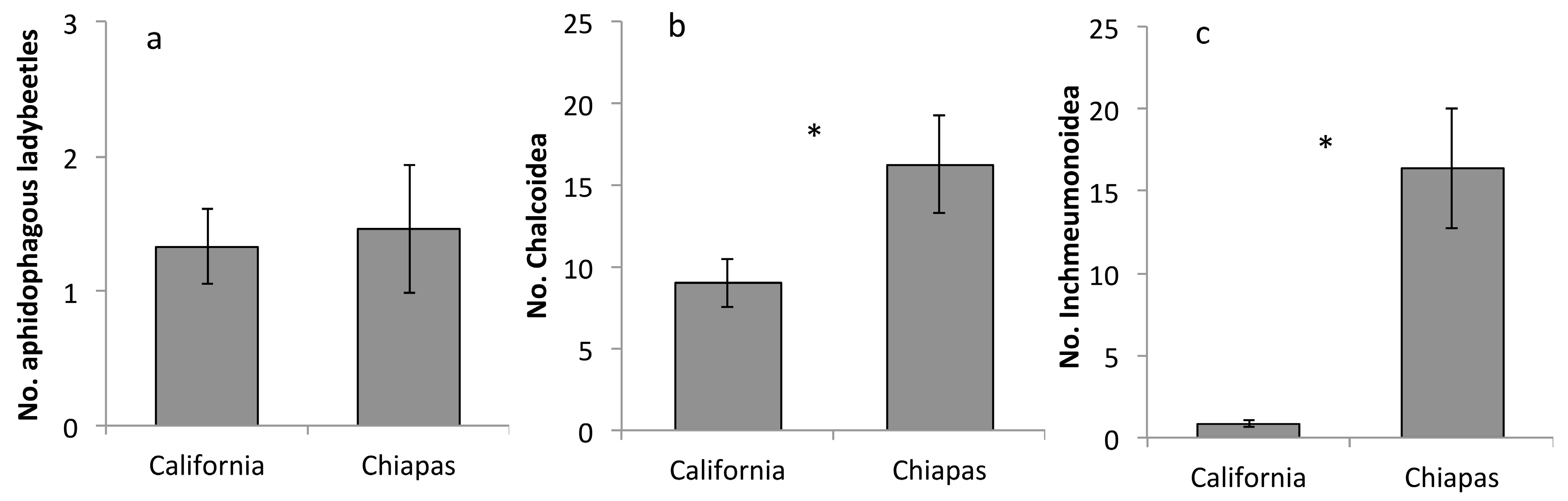
We collected a total of 40 aphidophagous ladybeetles. We collected 341 Chalcidoidea and 196 Ichneumonoidea parasitoids. Abundance of aphidophagous ladybeetles did not differ in California and Chiapas (t = 0.236, p = 0.828, Figure 1a). In contrast, abundance of both groups of parasitoids was higher in Chiapas. Chalcidoidea abundance was nearly twice as high in Chiapas (t = 2.408, p = 0.023, Figure 1b) and Ichneumonoidea abundance was more than eighteen times higher in Chiapas than in California (t = 5.453, p < 0.001, Figure 1c).
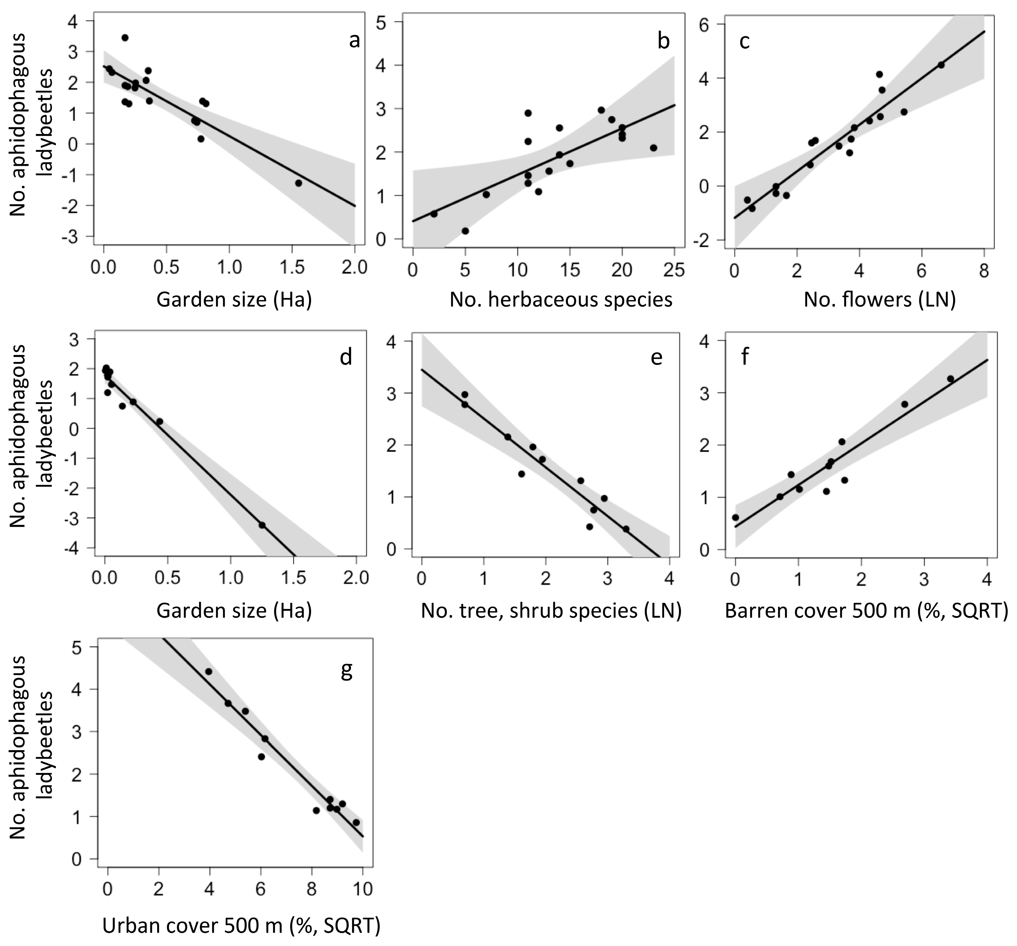
Several local and landscape characteristics correlated with higher or lower abundance of these natural enemy groups in the two locations. For California, the model that best predicted aphidophagous ladybeetle abundance was an average of the top eight models and included six local and two landscape factors. Ladybeetle abundance was higher in smaller gardens (p = 0.007, Figure 2a), with higher herbaceous plant species richness (p = 0.033, Figure 2b), and with higher floral abundance (p = 0.039, Figure 2c). Although included in top models, the abundance of ladybeetles did not differ with the number of tree and shrub species (p = 0.073), bare cover (p = 0.074), mulch cover (p = 0.128), urban cover within 500 m (p = 0.146) or open cover within 500 m (p = 0.157). For Chiapas, the model that best predicted ladybeetle abundance included two local factors and two landscape factors. Ladybeetles were more abundant in small gardens (p < 0.001, Figure 2d), with low tree and shrub richness (p < 0.001, Figure 2e), with more barren vegetation (p < 0.001, Figure 2f) and in sites with less urban cover (p < 0.001, Figure 2g).
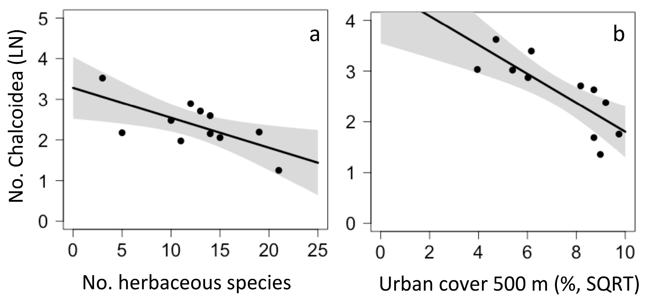
In California, the model that best predicted Chalcidoidea abundance was an average of eight top models that included garden age, garden size, mulch and herbaceous cover, and urban cover within 500 m; however, no factor significantly predicted Chalcidoidea abundance. In Chiapas, the model that best predicted Chalcidoidea abundance was the average of three top models and included two local factors and one landscape factor. Chalcidoidea abundance declined with the number of herbaceous plant species (p = 0.032, Figure 3a) and with urban cover in the surrounding landscape (p = 0.007, Figure 3b), but did not differ with changes in herbaceous cover (p = 0.089).
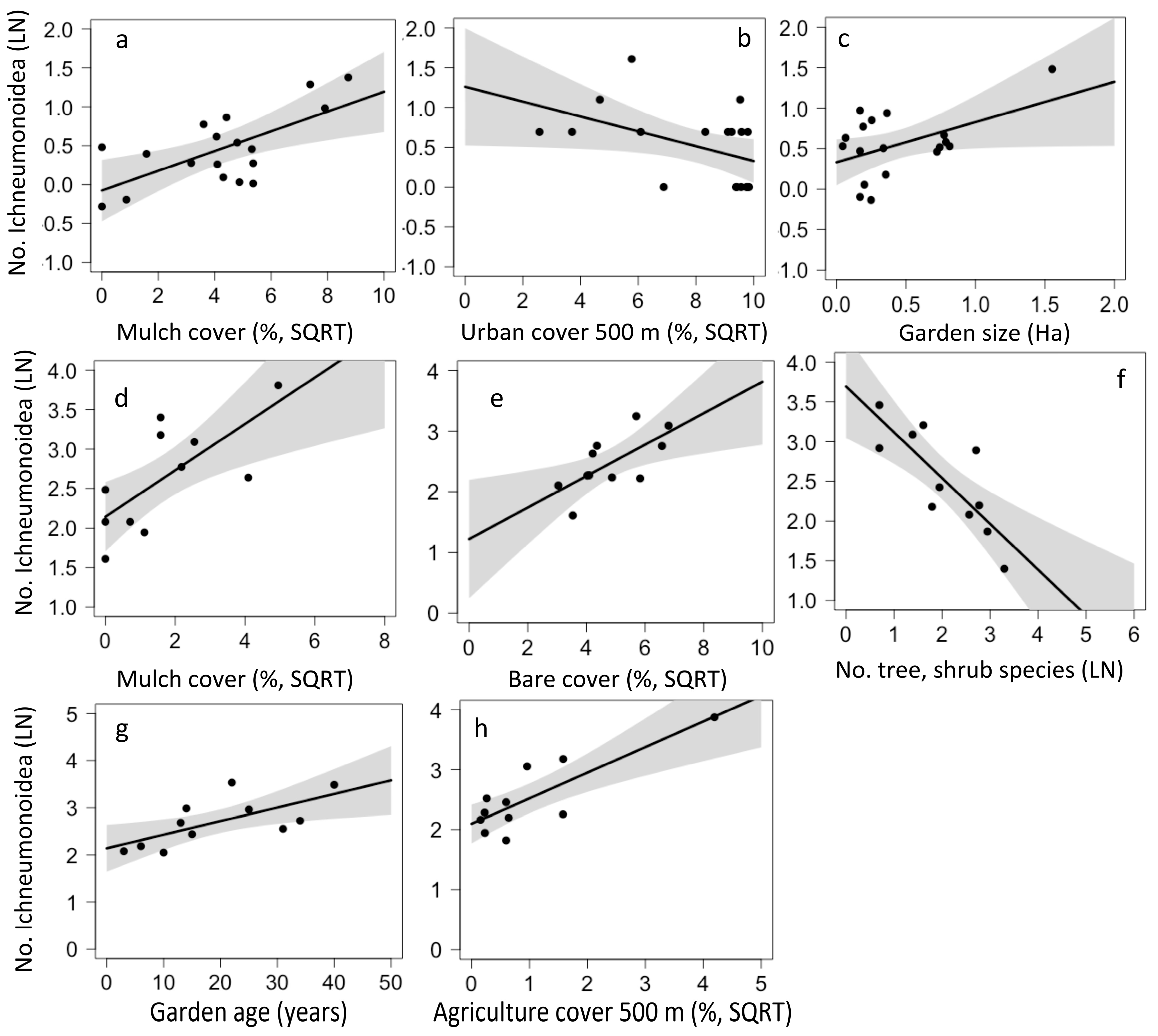
For California, the model that best predicted abundance of Ichneumonoidea was an average of the top four models and included one landscape and three local factors. For Chiapas, the model that best predicted Ichneumonoidea abundance included three local factors, one landscape factor, and garden age. Ichneumonoidea abundance increased with mulch cover in both California (p = 0.019, Figure 4a) and Chiapas (p = 0.008, Figure 4d). In California, abundance was lower in gardens with more urban cover (p = 0.057, Figure 4b) and higher in larger gardens (p = 0.048, Figure 4c). In Chiapas, Ichneumonoidea abundance was higher in gardens with more bare cover (p = 0.027, Figure 4e), in gardens fewer tree and shrub species (p = 0.001, Figure 4f), in gardens with more agriculture cover in the surrounding landscape (p = 0.002, Figure 4h) and in older gardens (p = 0.03, Figure 4g).
3.3. Prey Removal
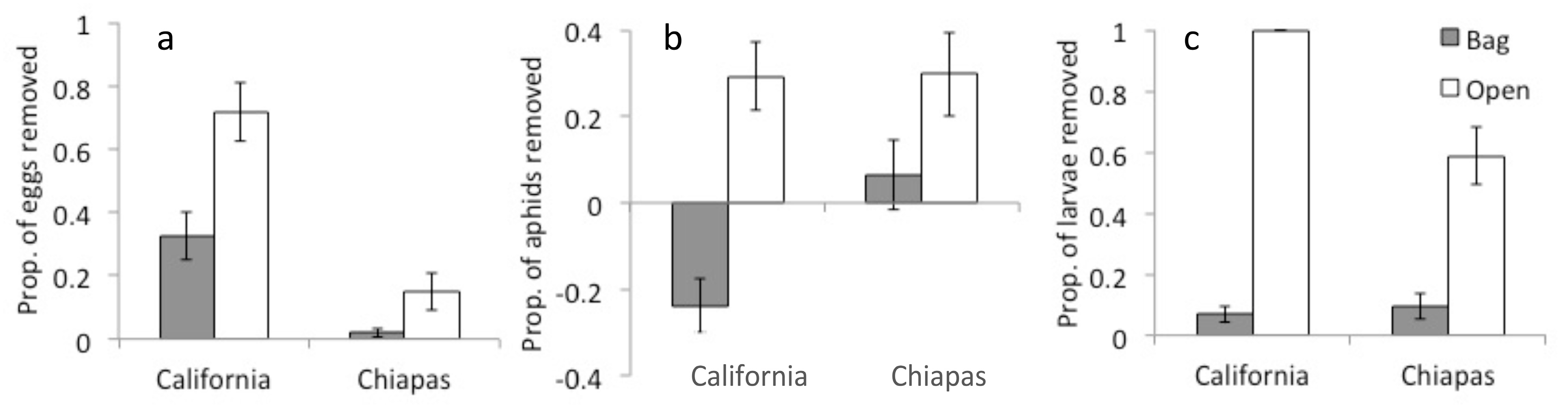
Natural enemies removed large proportions of prey items in both locations; on plants to which predators had access, they removed 15–72% of eggs (Figure 5a), nearly 30% of aphids (Figure 5b), and 58–100% of larvae (Figure 5c). According to the GLMM models, egg removal was higher in open compared with bagged treatments (t = 5.41, p < 0.001), and relative removal was higher in California than in Chiapas (t = 5.46, p < 0.001). Likewise, aphid removal was higher on open compared with bagged plants (t = 3.97, p < 0.001), but relative removal of eggs did not differ with location (t = 0.77, p = 0.446). Larvae removal was higher on open compared with bagged plants (z = 9.303, p < 0.001), and was higher in California than in Chiapas (z = 4.430, p < 0.001).
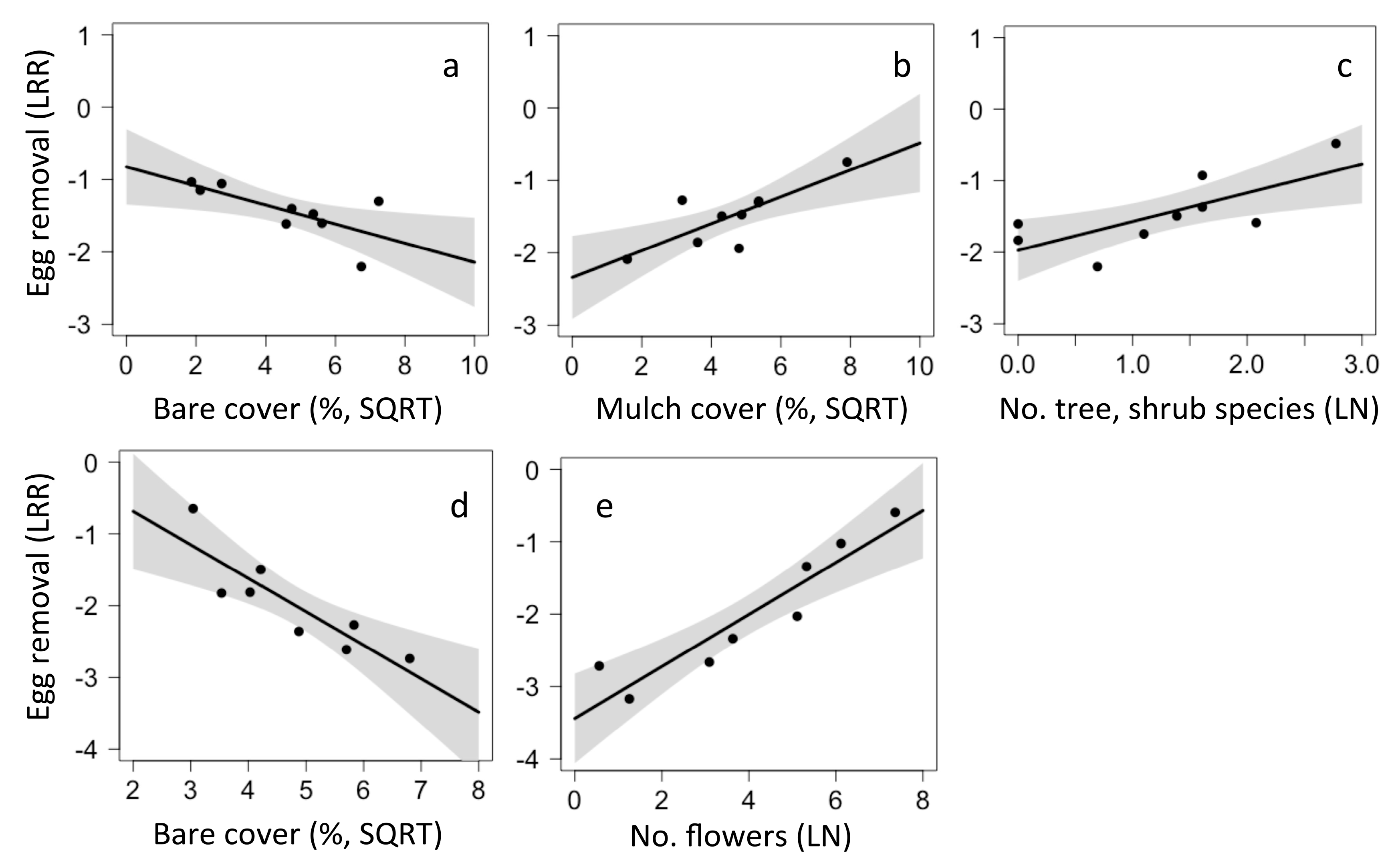
Egg and aphid removal were influenced by local factors, whereas larvae removal responded to both local and landscape factors. In California, the model that best predicted egg removal was an average of the top four models and included three local factors. Egg removal was higher in sites with less bare cover (p = 0.02, Figure 6a), more mulch (p = 0.026, Figure 6b), and with more tree and shrub species (p = 0.052, Figure 6c). In Chiapas, the model that best predicted egg removal was an average of three top models and included two local factors. Again, egg removal was lower in sites with high bare cover (p = 0.009, Figure 6d), but increased in sites with more flowers (p = 0.023, Figure 6e).
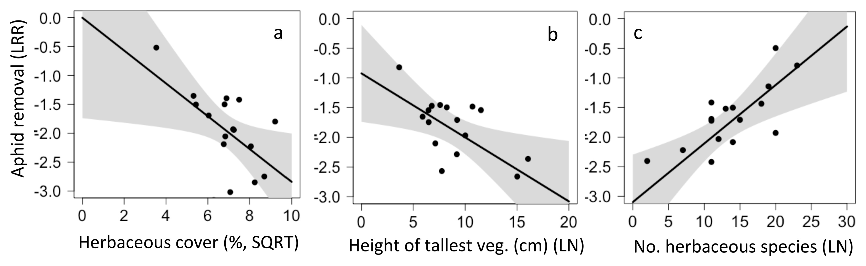
In California, the model predicting aphid removal was an average of the top four models and included five local factors. Aphid removal was higher in sites with less herbaceous cover (p = 0.042, Figure 7a), shorter herbaceous vegetation (p = 0.027, Figure 7b) and with higher herbaceous species richness (p = 0.029, Figure 7c); other factors in the model were not significant predictors. Aphid removal in Chiapas was not correlated with any local or landscape factors.
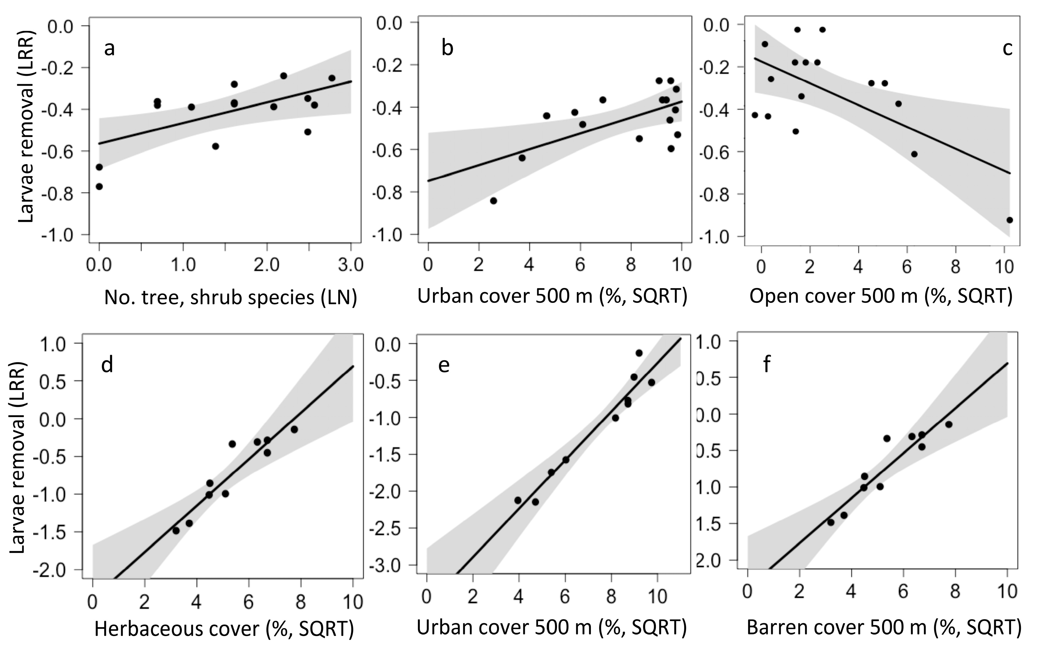
The best model for larvae removal in California included one local and two landscape factors. Larvae removal was higher in sites with more tree and shrub species (p = 0.021, Figure 8a), more urban cover (p = 0.024, Figure 8b), and more open cover (p = 0.021, Figure 8c). The model predicting larvae removal in Chiapas was an average of three top models and included one local and two landscape factors. Larvae removal was higher in sites with more herbaceous plant cover (p < 0.001, Figure 8d), more urban cover (p = 0.01, Figure 8e), and with more barren cover (p < 0.001, Figure 8f).
4. Discussion
Our experiments demonstrate that natural enemies are performing pest-control functions in both of our study regions. However, we found intriguing differences between California and Chiapas in the relative abundance of parasitoids. Furthermore, natural enemy abundance correlated with different site and landscape characteristics in the two regions. Our findings point to a need for further research to understand the mechanisms of local and landscape effects as well as simple interventions that are likely to favor natural enemy activity. We also identify some of the difficulties involved in comparative landscape ecology studies in general and international studies in particular.
4.1. Natural Enemies
Aphidophagous ladybeetles were equally numerous in California and Chiapas. At the site scale, their numbers decreased with garden size in both regions and with woody species richness in Chiapas while increasing in response to herbaceous species richness and flower abundance in California. An increase in woody richness may have provided more species of alternative prey (e.g., aphids) for ladybeetles in the trees, potentially lowering our ability to find ladybeetles in the herbaceous vegetation (the strata where our sampling took place). Increases in floral abundance may have provided more pollen and nectar resources, often food resources for ladybeetles, but promoting floral abundance to attract ladybeetles for biological control could be used with caution since increasing floral abundance may lower predation rate in some agricultural settings [36]. One other study in the same California sites noted lower ladybeetle species richness in smaller gardens [14]. Intriguingly, ladybeetle abundance did not respond to urban cover in California but was strongly inversely related to urban cover in Chiapas. Urban gardens may provide a sort of oasis for insects, especially during the dry season, when little green vegetation, prey resources, flowers, or water is available in the surrounding landscape [37]. The dry season in the Chiapas highlands is less extreme than California’s, and some resources for insects remain abundant in wetlands, fields, and other open areas as well as in gardens. Thus, the garden oasis effect, and thus the impact of urban cover may be stronger in California than in Chiapas. This difference in landscape context may also be related to differences in how we classified land use in the two regions. For California, we used the National Land Cover Data Base, which has 30 m resolution and categorizes pixels with as little as 20% impervious surface as urban. Hand digitizing land cover in Chiapas was at a smaller spatial scale. Thus, our “urban” category is likely to include much more green space in California than in Chiapas.
Ichneumonoidea were nearly 18 times more abundant in Chiapas, and Chalcidoidea were also significantly more abundant in Chiapas than in California. Chalcidoidea abundance did not respond to site or landscape variables in California but was inversely associated with herbaceous species richness and urban landscape cover in Chiapas. In both regions, Ichneumonoidea abundance was higher in sites with more mulch. Mulch has positive effects on parasitoid abundance in Australian vineyards [38], and on the abundance of different families and superfamilies of parasitoids in California study sites [13], but we do not know the mechanism that underlies this relationship. It is possible that mulch provides a hiding place for the parasitoids or that it provides more prey. Both Chalcidoidea and Ichneumonoidea abundance were negatively influenced by urban cover, which in this study is inversely related to natural cover and landscape diversity. Decreases in impervious surface [12] and increases in natural habitat and landscape diversity are often implicated as beneficial in studies of parasitoids [39,40]. Other predictors of Ichneumonoidea abundance differed between the two locations, with urban cover and garden size important in California and bare cover, number of trees and shrub species, garden age and agricultural cover in the landscape important in Chiapas. None of the predictor variables for either parasitoid taxon differed between the two regions in ways that could explain the higher parasitoid abundance we observed in Chiapas. Instead, these regional differences may be explained by biogeographical patterns in parasitoid distribution. Chalcidoidea species richness is higher in the tropics than in temperate zones [41]. Recent work shows that Ichneumonoidea may follow the same trend [42,43], challenging the idea that this taxa is more diverse at higher latitudes [44]. We did not identify wasps to the species level, but the abundance of wasps we observed in Chiapas may reflect the higher species richness of this taxon in the tropics. One important thing to note for these studies on natural enemy abundance, and particularly where we found strong differences, is that the timing of our study was quite limited (just one week in each location). Abundance of many natural enemies may differ dramatically seasonally in the two locations and should be more carefully considered in future studies.
4.2. Prey Removal
Prey removal rates were high in all locations with between 15–100% of sentinel prey removed within 24 h consistent with other studies that have examined prey removal in urban gardens [6,8]. In both locations, egg removal declined with more bare cover, and increased with factors associated with vegetation complexity (number of tree and shrub species, and number of flowers). Although we did not survey predator identity for any of the prey species used, in casual observations while collecting data, most predators observed on eggs were ants; in California in particular, these were the invasive Linepithema humile (Argentine ant). Egg removal decreased with increases in bare ground, and changes in bare ground or temperature may have impacted foraging of ants or other predators. Egg removal also increased with mulch cover, a factor that may be associated with higher activity density of spiders, another likely egg predator [22]. Egg removal also increased with higher vegetation complexity and in sites with higher floral abundance; both are factors that may increase the abundance of natural enemies in agricultural habitats [45].
For aphids, removal rates were higher in California than in Chiapas and in California, aphid removal differed with herbaceous vegetation cover, height, and richness. Ladybeetles are likely the most frequent predator of aphids in these gardens. Initial aphid densities on experimental plants in California were much higher than in Chiapas. Ladybeetles respond to a number of cues including plant volatiles, aphid alarm pheromones, and honeydew [46], thus higher densities of aphids may have attracted higher abundance of ladybeetles to those plants and augmented removal rates. Aphid removal increased with more herbaceous plant species; with more species there might be a higher diversity of prey items, thereby maintaining higher ladybeetle populations in the garden. Moreover, a high diversity of plants may contribute to biocontrol by supplying other food items, such as pollen and nectar for ladybugs [45,47]. In fact, we saw that both aphidophagous ladybeetle abundance and aphid removal were positively associated with higher herbaceous plant diversity in California. On the other hand, aphid removal decreased with higher herbaceous cover and taller herbaceous vegetation. In many cases, the complexity of the foraging habitat, including factors like plant size and morphology can influence predator-prey interactions [48,49,50]. Although we did not account specifically for the different plant types in our analysis, changes in the types of leaves and other architectural components of garden plots may have influenced the speed with which ladybeetles encountered the sentinel prey items.
Relative removal rates of larvae in open compared to bagged plants were also higher in California than in Chiapas. In short observations, spiders, vespid wasps, and birds removed most larvae, but we do not have any information about whether these groups of natural enemies differ in the two locations. Removal rates of larvae in Chiapas may have been lower due to differences in larval species used and specifically the potential unpalatability Leptophobia aripa larvae. This species feeds primarily on Brasicales and hence may sequestrate glucosinolates, toxic compounds for insects and birds, in its body, thus making the larvae not very palatable for wasps or birds [51]. Moreover, Leptophobia aripa larvae show characteristics such as gregarious behavior and aposematic behavior that strongly suggests unpalatability. In addition, we did not attempt to provide any barrier that would have prevented larvae from leaving experimental plants, and so it is possible those larvae that left plants voluntarily inflated prey removal numbers, or that the two larvae species left plants at different rates. In subsequent experiments with Trichoplusia ni larvae in California, we did place pots inside of water ‘moats’ to prevent larvae from leaving plants and found very few larvae either in the water or on the sides of pots; thus, predators may have still removed larvae from areas immediately surrounding pots in the experiment described here. Larvae removal increased with tree and shrub richness (and thus abundance) in California. The number and diversity of trees in urban areas can promote bird diversity and specifically can enhance the abundance of native and of insectivorous birds [52,53,54] which were one of the major predator groups seen removing larvae. Increased removal of larvae in gardens with greater herbaceous cover in Chiapas may be attributable to its favorable habitat for other natural enemies. At the landscape scale, larvae removal increased with urban cover in both regions, while also increasing with barren cover in Chiapas but declining in response to open cover in California. Open cover is characterized by lawn and golf courses, whereas some urban areas do contain trees and vegetation, which again, may promote bird abundance, and thus larvae removal. Barren cover, here characterized mainly by open quarries, provides very low habitat availability for birds, and bird abundance may be more concentrated in gardens with much barren cover nearby, potentially increasing larvae removal.
For all prey items, and for both locations, additional experimental manipulations and observations could easily be used to both understand how particular factors (e.g., mulch, floral abundance, vegetation complexity) influence the abundance of other predator species (e.g., syrphid larvae, neuropterans, staphylinids, dermapterans, spiders), prey encounter rates, predator foraging, which predators are actually removing prey species, and successful biological control of garden pests. In particular, studies could also measure parasitism rates in gardens, especially in locations where parasitoid abundance outweighs abundance of other natural enemies.
4.3. Recommendations
Overall, our findings are quite nuanced depending on the natural enemy group or prey species examined. For instance, garden size positively influenced parasitoid abundance but negatively affected ladybeetle abundance. Tree and shrub richness negatively affected natural enemy abundance but had a positive effect on egg and larvae removal. Herbaceous plant cover benefits both aphid and larvae removal but lowers parasitoid abundance. Herbaceous plant richness affected ladybeetle abundance and aphid removal, but negatively affected parasitoid abundance. Thus, there are few recommendations for management changes with universally beneficial effects across taxa and location from our study. Two factors were related with multiple beneficial impacts. First, we found that floral abundance had positive effects on both ladybeetle abundance and egg removal. Although increases in ladybeetle abundance might increase predation, increased floral abundance may detract from the impact of ladybeetles as predators [36]. Second, mulch cover increased the abundance of parasitoids in both locations and enhanced egg predation in California. So, one seemingly simple recommendation might be to increase mulch in gardens to enhance natural enemy abundance and predation. However, other studies have documented no effect of mulch on ladybeetle abundance [7], a negative association between aphid removal and mulch but a positive correlation between aphid removal and leaf-litter cover [8] and a positive response of parasitoid wasp abundance to mulch [13]. Mulch may increase aphid predation by providing a habitat for spiders [55]. Thus, mulch may be beneficial in only some cases. We postulate that the influence of mulch on pest prevention is likely non-linear and may vary with the type of mulch and the site and landscape context. However, mulch cover may negatively impact urban bees [23], thus mulch application must be considered in the light of impacts on other beneficial insects. In addition, we only conducted predation trials during the dry season in each location, and there may be strong seasonal effects of these different local and landscape factors on both natural enemy abundance and predation effects. All of these ideas merit further study.
5. Conclusions
Our study confirms that the potential efficacy of conservation biological control extends to tropical cities. However, biocontrol agents and the site and landscape factors influencing their activity differ markedly between our study regions. Thus, as agroecologists have repeatedly affirmed [56], attempts to define universally applicable management practices are likely to be counterproductive. Instead, we need more comparative work to continue to develop our understanding of the general principals governing conservation biological control in urban settings, as well as local studies designed to refine geographically specific management recommendations. Knowledge exchange within networks of urban growers, perhaps modeled on farmer-to-farmer methodology [57], may help accelerate advancement of principles and practice. Dialog among growers and scientists will also be key to ensuring constant feedback between theory and practice [58]. Physical proximity between research institutions and urban growers, along with urban dweller’s relative ease of access to Internet data-sharing platforms (e.g., CitSci.org), may help accelerate these processes.
Author Contributions
Conceptualization, H.M., B.G.F., and S.M.P.; Methodology, H.M., B.G.F., D.N.G., S.M.P. and P.B.; Formal Analysis, L.E.M., S.M.P., and D.N.G.; Investigation, H.M., B.G.F, L.E.M., P.B., and S.M.P.; Resources, H.M. and S.M.P.; Data Curation, H.M., B.G.F., L.M., P.B., and S.M.P.; Writing—Original Draft Preparation, H.M., B.G.F., L.E.M., and S.M.P.; Writing—Review & Editing, H.M., B.G.F., L.E.M., P.B., and S.M.P.; Project Administration, H.M. and S.M.P.; Funding Acquisition, H.M. and S.M.P.
Funding
Funding for the research was provided by a UC-MEXUS-CONACYT Collaborative Grant to SMP and HM, Ruth and Alfred Heller Chair Funds from UCSC, a Committee on Research Faculty Research Grant from UCSC to SMP in 2015, and USDA-NIFA Award 2016-67019-25185.
Acknowledgments
Y. Bravo, J. Burks, H. Cohen, M. Egerer, A. García, M. MacDonald, M.E. Narvaez Cuellar, M. Otoshi, M. Plascencia, R. Quistberg, G. Santíz Ruíz, R. Schreiber-Brown, and S-S. Thomas assisted with data collection in the field and lab. We thank the UCSC Greenhouse staff J. Velzy and M. Dillingham for growing fava plants. We thank the following gardens and organizations for providing access for our research in California: Aptos Community Garden, City of San Jose Parks and Recreation (Berryessa Community Garden, El Jardin Community Garden, La Colina Community Garden, Coyote Creek Community Garden, Laguna Sega Community Garden), City of Santa Cruz Parks and Recreation (Trescony Garden and Beach Flats Garden), Homeless Garden Project, Live Oak Green Grange Community Garden, MEarth, Mesa Verde Gardens, Middlebury Institute of International Studies, Salinas Chinatown Community Garden, Santa Clara University Forge Garden, Seaside Giving Garden, and the Farm and Chadwick Garden on the UC Santa Cruz campus. We thank the following gardeners and organizations for providing access for our research in Chiapas: Antonio Saldivar, Kess Grootenboer, Marcos Ferguson Morales, María del Carmen Altuzar, Ron Nigh, Casa Lily, Escuela Primaria Josefa Ortíz de Dominguez, Casa del Pan, Convento Madres Clarisas, Huerto de ECOSUR and La Albarrada.
Conflicts of Interest
The authors declare no conflict of interest.
References
- Altieri, M. Agroecology: The Science of Sustainable Agriculture; CRC Press: Boca Ratón, FL, USA, 2018; p. 448. [Google Scholar]
- FAO. FAO‘s Work on Agroecology: A Pathway to Achieving the SDGs; I9021EN/1/03.18; FAO: Rome, Italy, 2018. [Google Scholar]
- Morales, H. Pest management in traditional tropical agroecosystems: Lessons for pest prevention research and extension. Integr. Pest Manag. Rev. 2002, 7, 145. [Google Scholar] [CrossRef]
- Tscharntke, T.; Bommarco, R.; Clough, Y.; Crist, T.; Kleijn, D.; Rand, T.; Thlianakis, J.; van Nouhuys, S.; Vidal, S. Conservation biological control and enemy diversity on a landscape scale. Biol. Control 2007, 43, 294–309. [Google Scholar] [CrossRef]
- Oberholtzer, L.; Dimitri, C.; Pressman, A. Urban agriculture in the United States: Characteristics, challenges, and technical assistance needs. J. Ext. 2014, 52. [Google Scholar] [CrossRef]
- Gardiner, M.; Praizner, S.; Burkman, C.; Albro, S.; Grewal, P. Vacant land conversion to community gardens: Influences on generalist arthropod predators and biocontrol services in urban greenspaces. Urban Ecosyst. 2014, 17, 101–122. [Google Scholar] [CrossRef]
- Egerer, M.; Arel, C.; Otoshi, M.; Quistberg, R.; Bichier, P.; Philpott, S. Urban arthropods respond variably to changes in landscape context and spatial scale. J. Urban Ecol. 2017, 3. [Google Scholar] [CrossRef] [Green Version]
- Philpott, S.; Bichier, P. Local and landscape drivers of predation services in urban gardens. Ecol. Appl. 2017, 27, 966–976. [Google Scholar] [CrossRef] [PubMed] [Green Version]
- McDonnell, M.; Breuste, J.; Hahs, A. Introduction: Scope of the book and need for developing comparative approach to the ecological study of cities and towns. In Ecology of Cities and Towns: A Comparative Approach; McDonnell, M., Hahs, A., Brueste, J., Eds.; Cambridge University Press: Cambridge, UK, 2009; p. 746. [Google Scholar]
- Pardee, G.; Philpott, S. Native plants are the bee’s knees: Local and landscape predictors of bee richness and abundance in backyard gardens. Urban Ecoyst. 2014, 17, 641–659. [Google Scholar] [CrossRef]
- Sperling, C.; Lortie, C. The importance of urban backgardens on plant and invertebrate recruitment: A field microcosm experiment. Urban Ecosyst. 2010, 13, 223–235. [Google Scholar] [CrossRef]
- Bennett, A.; Gratton, C. Local and landscape scale variables impact parasitoid assemblages across an urbanization gradient. Landsc. Urban Plan. 2012, 104, 26–33. [Google Scholar] [CrossRef]
- Burks, J.; Philpott, S. Local and landscape drivers of parasitoid abundance, richness, and composition in urban gardens. Environ. Entomol. 2017, 46, 201–209. [Google Scholar] [CrossRef] [PubMed]
- Egerer, M.; Bichier, P.; Philpott, S. Landscape and local habitat correlates of lady beetle abundance and species richness in urban agriculture. Ann. Entomol. Soc. Am. 2016, 110, 97–103. [Google Scholar] [CrossRef]
- Gardiner, M.; Landis, D.; Graton, C.; DiFonzo, C.; O’Neal, M.; Chacon, J.; Wayo, M.; Schmidt, N.; Meuller, E.; Heimpel, G. Landscape diversity enhances biological control of an introduced crop pest in the North-Central US. Ecol. Appl. 2009, 19, 143–154. [Google Scholar] [CrossRef] [PubMed]
- Burkman, C.; Gardiner, M. Urban greenspace compositionand landscape context influence natural enemy community composition and function. Biol. Control 2014, 75, 58–67. [Google Scholar] [CrossRef]
- Lin, B.; Philpott, S.; Jha, S. The future of urban agriculture and biodiversity-mediated ecosystem services: Challenges and next steps. Basic Appl. Ecol. 2015, 16, 189–201. [Google Scholar] [CrossRef]
- Mooney, H.; Zavaleta, E. Ecosystems of California; University of California Press: Oakland, CA, USA, 2016. [Google Scholar]
- U.S. Climate Data. Available online: https://www.usclimatedata.com/ (accessed on 19 April 2018).
- Datos Climáticos Mundiales. Available online: https://es.climate-data.org/ (accessed on 15 April 2018).
- Morales, H.; Vázquez, L.B.; Ferguson, B.G.; Díaz, B.M. Sembrando soberanía alimentaria en un mar de cemento: Retos y oportunidades de la agricultura urbana de Jovel. In Tópicos Socio-Ambientales Emergentes y Productivos en la Cuenca de Jovel y su Periferia; García, A., Soares, D., Eds.; Universidad Autonoma de Chapingo: Texcoco, Mexico, 2015. [Google Scholar]
- Otoshi, M.; Bichier, P.; Philpott, S. Local and landscape correlates of spider activity density and species richness in urban gardens. Environ. Entomol. 2015, 44, 1043–1051. [Google Scholar] [CrossRef] [PubMed]
- Quistberg, R.; Bichier, P.; Philpott, S. Landscape and local correlates of bee abundance and species richness in urban gardens. Environ. Entomol. 2016, 54, 592–601. [Google Scholar] [CrossRef] [PubMed]
- Homer, C.G.; Dewitz, J.A.; Yang, L.; Jin, S.; Danielson, P.; Xian, G.; Coulston, J.; Herold, N.D.; Wickham, J.D.; Megown, K. Completion of the 2011 National Land Cover Database for the conterminous United States—Representing a decade of land cover change information. Photogramm. Eng. Remote Sens. 2015, 81, 345–354. [Google Scholar] [CrossRef]
- INEGI Censo de Población y Vivienda 2010. México. Available online: http://www.inegi.org.mx/ (accessed on 18 April 2018).
- Oksanen, J. Multivariate Analysis of Ecological Communities in R; Vegan Tutorial; University Oulu: Oulu, Finland, 2015. [Google Scholar]
- McGarigal, K.; Cushman, S.; Neel, M.; Ene, E. FRAGSTATS v3: Spatial Pattern Analysis Program for Categorical Maps. Computer Software Program Produced by the Authors at the University of Massachusetts, Amherst, Massachusetts, USA. Available online: http://www.umass.edu/landeco/research/fragstats/fragstats.html (accessed on 12 January 2018).
- Discover Life. Available online: http://www.discoverlife.org (accessed on 15 October 2015).
- Gordon, R.D. The Coccinellidae (Coleoptera) of America north of Mexico. J. N. Y. Entomol. Soc. 1985, 93, 1–912. [Google Scholar]
- Goulet, H.; Huber, J. Hymneoptera of the World: An Identification Guide to Families; Centre for Land and Biological Resources Research: Ottawa, ON, Canada, 1993. [Google Scholar]
- R Development Core Team. A Language and Environment for Statistical Computing; R Foundation for Statistical Computing: Vienna, Austria, 2017. [Google Scholar]
- Pinheiro, J.; Bates, D.; Debroy, S.; Sarkar, D.; R Development Core Team. nlme: Linear and Ninlinear Mixed Effects Models. R Package Version 3.1-137. 2018. Available online: https://CRAN.R-project.org/package=nlme (accessed on 15 March 2018).
- Calcagno, V.; de Mazancourt, C. glmulti: An R package for easy automated model selection with (generalized) linear models. J. Statain. Softw. 2010, 34, 1–29. [Google Scholar] [CrossRef]
- Barton, K. MuMin: Multi-Model Inference. R Package Version 1.5.2. Available online: https://cran.r-project.org/web/packages/MuMIn/MuMIn.pdf (accessed on 14 June 2015).
- Breheny, P.; Burchett, W. Visualization of Regression Models Using Visreg. Available online: http://myweb.uiowa.edu/pbreheny/publications/visreg.pdf (accessed on 18 June 2015).
- Jonsson, M.; Wratten, S.; Landis, D.; Tompkins, J.-M.; Cullen, R. Habitat manipulation to mitigate the impacts of invasive arthropod pests. Biol. Invasions 2010, 12, 2933–2945. [Google Scholar] [CrossRef] [Green Version]
- Marín, L.; Morales, H.; Martínez-Sánchez, M.; Sago, P.; Navarrete, D. Floral visitors in urban gardens and natural areas: Diversity and interaction networks in a neotropical urban landscape. Unpublished work. 2018. [Google Scholar]
- Thomson, L.; Hoffmann, A. Effects of ground cover (straw and compost) on the abundance of natural enemies and soil macro invertebrates in vineyards. Agric. For. Entomol. 2007, 9, 173–179. [Google Scholar] [CrossRef]
- Letourneau, D.; Bothwell Allen, S.; Stireman, J. Perennial habitat fragments, parasitoid diversity, and parasitism in ephemeral crops. J. Appl. Ecol. 2012, 49, 1405–1416. [Google Scholar] [CrossRef]
- Brewer, M.; Noma, T.; Elliott, N.; Kravchenko, A.; Hild, A. A landscape view of cereal aphid parasitoid dynamics reveals sensitivity to farmand region-scale vegetation structure. Eur. J. Entomol. 2008, 105, 503–511. [Google Scholar] [CrossRef]
- Noyes, J. The diversity of Hymenoptera in the tropics with special reference to Parasitica in Sulawesi. Ecol. Entomol. 1989, 14, 197–207. [Google Scholar] [CrossRef]
- Veijalainen, A.; Wahlberg, N.; Broad, G.R.; Erwin, T.L.; Longino, J.T.; Saaksjarvi, I.E. Unprecedented ichneumonid parasitoid wasp diversity in tropical forests. Proc. R. Soc. Lond. B Biol. 2012, 279, 4694–4698. [Google Scholar] [CrossRef] [PubMed] [Green Version]
- Eagalle, T.; Smith, M. Diversity of parasitoid and parasitic wasps across a latitudinal gradient: Using public DNA records to work within a taxonomic impediment. FACETS 2017, 2, 937–954. [Google Scholar] [CrossRef] [Green Version]
- Janzen, D. The Peak in North American ichneumonid species richness lies between 38 degrees and 42 degrees N. Ecology 1981, 62, 532–537. [Google Scholar] [CrossRef]
- Andow, D. Vegetational diversity and arthropod population response. Annu. Rev. Entomol. 1991, 36, 561–586. [Google Scholar] [CrossRef]
- Hodek, I.; Hodek, A. Ecology of Coccinellidae; Kluwer Academic: Dordrecht, The Netherlands, 1996. [Google Scholar]
- Iverson, A.; Marín, L.; Ennis, K.; Gonthier, D.; Connor-Barrie, B.; Remfert, J.; Cardinale, B.; Perfecto, I. Do polycultures promote win-wins or trade-offs in agricultural ecosystem services? A meta-analysis. J. Appl. Ecol. 2014, 51, 1593–1602. [Google Scholar] [CrossRef] [Green Version]
- Šipoš, J.; Kindlmann, P. Effect of the canopy complexity of trees on the rate of predation of insects. J. Appl. Ecol. 2012, 137, 445–451. [Google Scholar] [CrossRef]
- Langellotto, G.; Denno, R. Responses of invertebrate natural enemies to complex-structured habitats: A meta-analytical synthesis. Oecologia 2004, 139, 1–10. [Google Scholar] [CrossRef] [PubMed]
- Legrand, A.; Barbosa, P. Plant morphological complexity impacts foraging efficiency of adult Coccinella septempunctata L. (Coleoptera: Coccinellidae). Environ. Entomol. 2003, 32, 1219–1226. [Google Scholar] [CrossRef]
- Wheat, C.; Vogel, H.; Wittstock, U.; Braby, M.; Underwood, D.; Mitchell-Olds, T. The genetic basis of a plant–insect coevolutionary key innovation. Proc. Natl. Acad. Sci. USA 2007, 104, 20427–20431. [Google Scholar] [CrossRef] [PubMed]
- Barth, B.; FitzGibbon, S.; Wilson, R. New urban developments that retain more remnant trees have greater bird diversity. Landsc. Urban Plan. 2015, 136, 122–129. [Google Scholar] [CrossRef]
- Ortega-Álvarez, R.; MacGregor-Fors, I. Living in the big city: Effects of urban land-use on bird community struture, diversity, and composition. Landsc. Urban Plan. 2009, 90, 189–195. [Google Scholar] [CrossRef]
- White, J.; Antos, M.; Fitzsimons, J.; Palmer, G. Non-uniform bird assemblages in urban environments: The influence of streetscape vegetation. Landsc. Urban Plan. 2005, 71, 123–135. [Google Scholar] [CrossRef]
- Schmidt, M.H.; Thewes, U.; Thies, C.; Tscharntke, T. Aphid suppression by natural enemies in mulched cereals. Entomol. Exp. Appl. 2004, 113, 87–93. [Google Scholar] [CrossRef]
- Rosset, P.; Altieri, M. Agroecology: Science and Politics; Fernwood Publishing: Black Point, NS, Canada, 2017; p. 160. [Google Scholar]
- Holt Gimenez, E. Campesino a Campesino, Voices from Latin America, Farmer to Farmer Movement for Sustainable Agriculture; Food First Books: Oakland, CA, USA, 2006. [Google Scholar]
- Vandermeer, J.; Perfecto, I. Complex traditions: Intersecting theoretical frameworks in agroecological research. Agroecol. Sustain. Food 2013, 37, 76–89. [Google Scholar] [CrossRef]
Figure 1.
Differences in abundance (mean ± standard Error) for aphidophagous ladybeetles (a), Chalcidoidea parasitoids (b), and (c) Ichneumonoidea parasitoids in urban gardens in the central coast of California (USA) and in in the Chiapas highlands (Mexico). Asterisks (*) indicate significant differences in mean abundance in the two different locations as determined with t-tests (see text for details).

Figure 2.
Local and landscape drivers of aphidophagous ladybeetle abundance in urban gardens in the central coast of California (a–c) and in the Chiapas highlands (d–g).
Figure 2.
Local and landscape drivers of aphidophagous ladybeetle abundance in urban gardens in the central coast of California (a–c) and in the Chiapas highlands (d–g).

Figure 3.
Local and landscape drivers of Chalcidoidea abundance in urban gardens in Chiapas (a,b). There were no significant predictors of Chalcidoidea abundance in California.
Figure 3.
Local and landscape drivers of Chalcidoidea abundance in urban gardens in Chiapas (a,b). There were no significant predictors of Chalcidoidea abundance in California.

Figure 4.
Local and landscape drivers of Ichneumonoidea abundance in urban gardens in California (a–c) and in Chiapas (d–h).
Figure 4.
Local and landscape drivers of Ichneumonoidea abundance in urban gardens in California (a–c) and in Chiapas (d–h).

Figure 5.
Proportions of eggs (a), aphids (b), and moth larvae (c) missing from open (predator access) and bagged (predator exclosure) plants in urban gardens in California and Chiapas.
Figure 5.
Proportions of eggs (a), aphids (b), and moth larvae (c) missing from open (predator access) and bagged (predator exclosure) plants in urban gardens in California and Chiapas.

Figure 6.
Local and landscape drivers of egg removal in California (a–c) and Chiapas (d–e).

Figure 7.
Local and landscape drivers of aphid removal (a–c) in California. No factors significantly predicted aphid removal in Chiapas.
Figure 7.
Local and landscape drivers of aphid removal (a–c) in California. No factors significantly predicted aphid removal in Chiapas.

Figure 8.
Local and landscape drivers of larvae removal in California (a–c) and Chiapas (d–f).


Table 1.
Local and landscape characteristics of urban garden study sites in the Central Coast of California (USA) and the Chiapas highlands (Mexico). All values show mean ± standard error, and statistical results are for independent sample t-tests comparing values between the two locations.
Table 1.
Local and landscape characteristics of urban garden study sites in the Central Coast of California (USA) and the Chiapas highlands (Mexico). All values show mean ± standard error, and statistical results are for independent sample t-tests comparing values between the two locations.
| Predictor Variables | California | Chiapas | t-Stat | p-Value |
|---|---|---|---|---|
| No. of gardens | 18 | 11 | NA | NA |
| Garden age (years) | 19.11 ± 3.34 | 19.36 ± 3.61 | −0.049 | 0.961 |
| Garden size (hectares) | 0.44 ± 0.38 | 0.20 ± 0.37 | 1.647 | 0.111 |
| Canopy cover (%) | 9.33 ± 2.82 | 25.54 ± 7.84 | −2.374 | 0.025 |
| No. trees and shrubs | 18.5 ± 6.08 | 39.91 ± 9.15 | −2.245 | 0.033 |
| No. tree and shrub species | 4.89 ± 1.11 | 9.55 ± 2.43 | −1.77 | 0.088 |
| No. trees and shrubs in flower | 5.56 ± 1.77 | 10.91 ± 3.6 | −1.294 | 0.207 |
| Tallest non-woody vegetation (cm) | 88.42 ± 15.22 | 47.66 ± 8.32 | 2.165 | 0.039 |
| No. herbaceous plant species | 13.67 ± 1.33 | 12.45 ± 1.6 | 0.573 | 0.571 |
| Bare cover (%) | 30.15 ± 4.78 | 24.66 ± 3.77 | 0.455 | 0.653 |
| Grass cover (%) | 3.71 ± 1.26 | 22.0 ± 7.07 | −2.66 | 0.013 |
| Herbaceous cover (%) | 48.07 ± 4.25 | 32.75 ± 4.94 | 2.328 | 0.028 |
| Mulch cover (%) | 23.51 ± 5.06 | 5.39 ± 2.41 | 2.971 | 0.006 |
| Rock cover (%) | 4.0 ± 2.43 | 5.07 ± 1.73 | −0.841 | 0.408 |
| Leaf litter cover (%) | 9.83 ± 4.3 | 14.48 ± 6.28 | −0.749 | 0.461 |
| No. flowers | 87.99 ± 41.31 | 259.55 ± 139.46 | −1.178 | 0.249 |
| Natural land cover (%) | 12.08 ± 4.47 | 38.3 ± 8.13 | −3.075 | 0.005 |
| Urban land cover (%) | 68.45 ± 7.57 | 56.39 ± 8.57 | 1.023 | 0.315 |
| Agriculture land cover (%) | 2.6 ± 1.8 | 2.26 ± 1.56 | 0.133 | 0.895 |
| Barren land cover (%) | NA | 3.06 ± 1.04 | NA | NA |
| Open land cover (%) | 16.17 ± 4.06 | NA | NA | NA |
| Landscape diversity H | 1.17 ± 0.07 | 1.06 ± 0.13 | 0.774 | 0.446 |
Landscape variables were measured in 500 m buffers in California and in Chiapas. NA means not applicable, no value was recorded or no test was conducted.
Table 2.
Lists of variables selected for analysis and those variables with which they were correlated. PCC shows the Pearson correlation coefficients between variables, and the sign (+/−) shows direction of correlation.
Table 2.
Lists of variables selected for analysis and those variables with which they were correlated. PCC shows the Pearson correlation coefficients between variables, and the sign (+/−) shows direction of correlation.
| Selected Variable | Correlated Variable | PCC |
|---|---|---|
| Garden age (years) | NA | NA |
| Garden size (hectares) | NA | NA |
| Height of tallest vegetation (sqrt of cm) | NA | NA |
| No. herbaceous plant species | NA | NA |
| No. flowers (LN) | NA | NA |
| No. tree and shrub species (LN) | Canopy cover (sqrt of %) | 0.677 |
| No. trees and shrubs (LN) | 0.872 | |
| No. trees and shrubs in flower (LN) | 0.908 | |
| Herbaceous cover (sqrt of %) | Grass cover (sqrt of %) | −0.401 |
| Rock cover (sqrt of %) | −0.376 | |
| Leaf litter cover (sqrt of %) | 0.617 | |
| Bare cover (sqrt of %) | NA | NA |
| Mulch cover (sqrt of %) | NA | NA |
| Urban land cover in 500 m (sqrt of %) | Natural land cover in 500 m (sqrt of %) | −0.822 |
| Landscape diversity H | −0.536 | |
| Agriculture land cover of 500 m (sqrt of %) | Landscape diversity H | 0.445 |
| Open land cover in 500 m (sqrt of %) | NA | NA |
| Barren land cover in 500 m (sqrt of %) | NA | NA |
Sqrt is square root; LN is natural log. NA means not applicable, no variable was correlated with the selected variable.
© 2018 by the authors. Licensee MDPI, Basel, Switzerland. This article is an open access article distributed under the terms and conditions of the Creative Commons Attribution (CC BY) license (http://creativecommons.org/licenses/by/4.0/).
Share and Cite
MDPI and ACS Style
Morales, H.; Ferguson, B.G.; Marín, L.E.; Gutiérrez, D.N.; Bichier, P.; Philpott, S.M. Agroecological Pest Management in the City: Experiences from California and Chiapas. Sustainability 2018, 10, 2068. https://doi.org/10.3390/su10062068
AMA Style
Morales H, Ferguson BG, Marín LE, Gutiérrez DN, Bichier P, Philpott SM. Agroecological Pest Management in the City: Experiences from California and Chiapas. Sustainability. 2018; 10(6):2068. https://doi.org/10.3390/su10062068
Chicago/Turabian StyleMorales, Helda, Bruce G. Ferguson, Linda E. Marín, Dario Navarrete Gutiérrez, Peter Bichier, and Stacy M. Philpott. 2018. "Agroecological Pest Management in the City: Experiences from California and Chiapas" Sustainability 10, no. 6: 2068. https://doi.org/10.3390/su10062068
Note that from the first issue of 2016, this journal uses article numbers instead of page numbers. See further details here.