Leading El-Niño SST Oscillations around the Southern South American Continent


1
Department of Marine Environment and Engineering, National Sun Yat-Sen University, Kaohsiung 80424, Taiwan
2
Taiwan Ocean Research Institute, National Applied Research Laboratories, Kaohsiung 80143, Taiwan
3
Department of Earth Sciences, National Taiwan Normal University, Taipei 11677, Taiwan
*
Authors to whom correspondence should be addressed.
Sustainability 2018, 10(6), 1783; https://doi.org/10.3390/su10061783
Submission received: 20 April 2018
/
Revised: 19 May 2018
/
Accepted: 28 May 2018
/
Published: 29 May 2018
(This article belongs to the Section Environmental Sustainability and Applications)
Abstract
:The inter-annual variations in the sea surface temperatures (SSTs) of the tropical and subtropical Pacific Ocean have been widely investigated, largely due to their importance in achieving the sustainable development of marine ecosystems under a changing climate. The El Niño-Southern Oscillation (ENSO) is a widely recognized variability. In the subpolar region in the southern hemisphere, the Antarctic Circumpolar Current (ACC) is one of the main sources of the Peru Current. A change in the SST in the Southern Ocean may change the physical properties of the seawater in the tropical and subtropical Pacific Ocean. However, the variations in the SST in the Southern Ocean have rarely been addressed. This study uses a 147-year (1870–2016) dataset from the Met Office Hadley Centre to show that the SST anomalies (SSTAs) in the oceans west and east of South America and the Antarctic Peninsula have strong positive (R = 0.56) and negative (R = −0.67) correlations with the Niño 3.4 SSTA, respectively. Such correlations are likely related to the changes in circulations of the ACC. We further show that, statistically, the temporal variations in the SSTAs of the ACC lead the Niño 3.4 SSTA by four to six months. Such findings imply that change in the strength of ENSO or circulation under the changing climate could change the climate in regions at higher latitudes as well.
1. Introduction
Without the influence of marginal barriers, the Drake Passage establishes the strongest and longest current in the oceans, the Antarctic Circumpolar Current (ACC). The ACC has a volume transport of approximately 130–140 Sv (1 Sv ≅ 106 m3 s−1), extending around the globe to a length of approximately 24,000 km. The ACC connects the Atlantic, Pacific, and Indian Oceans, serving as a conduit for all active and passive oceanic tracers, notably heat and salt, which affect the Earth’s climate, oceanic mass stratification, circulation, as well as air-sea heat and mass exchanges [1]. For instance, the intensity of the ACC strongly affects the marine ecosystems and sea surface temperature (SST) in the Southwest Atlantic Ocean [2,3,4,5]. However, largely due to its remoteness and harsh environmental conditions, the Southern Ocean is relatively poorly sampled and investigated [6].
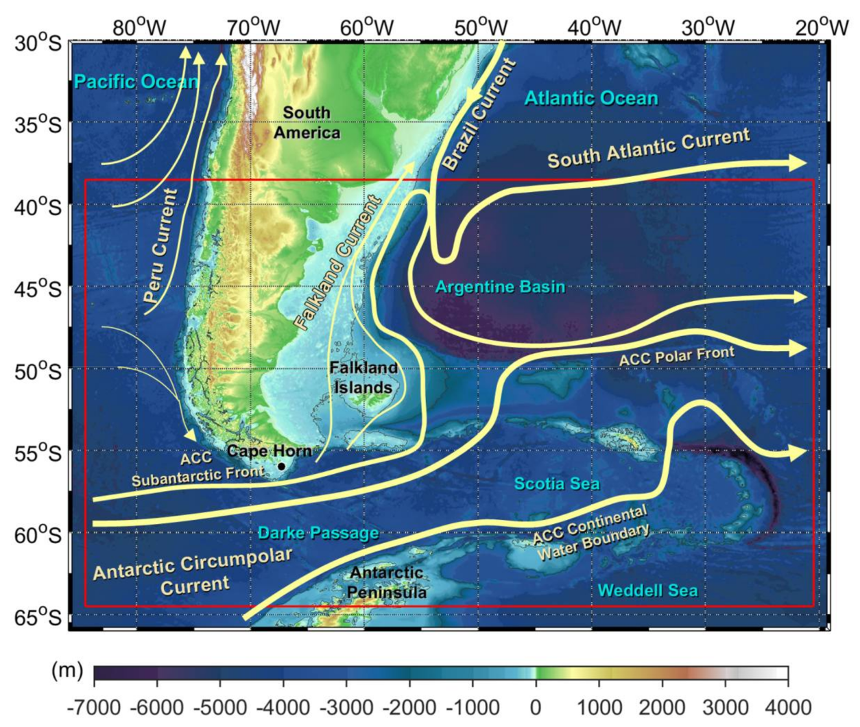
South America and the Falkland Islands are major constraining landforms for the ACC and Falkland Current (FC, also known as the Malvinas Current), forming a complex hydrographic system. In the Southwest Atlantic Ocean, the Patagonian Shelf, where the surface ocean circulation is dominated by the opposing flows of the Brazil Current (BC) and the FC [7], is also a region with a complex pattern of currents (Figure 1). In the regions where these two currents meet, the BC flows southward along the continental slope, carrying subtropical warm and salty water to the South-Atlantic anticyclonic gyre [8]. The FC is a detachment of the ACC that flows northward with distinguishable low temperatures [9]. At approximately 38° S, these two currents meet and generate a quasi-stationary meander that extends northward to approximately 45° S [10]. This quasi-stationary meander zone is the so-called Brazil-Malvinas Confluence (BMC) region, which is one of the most dynamically active regions in the world oceans [11].
It has been widely recognized that the El Niño-Southern Oscillation (ENSO) causes significant inter-annual climate variations in the Northern Pacific. The influences extend as far as South America [12,13,14,15,16,17,18,19]. Generally, the differences in the responses to ENSO in the Southern Hemisphere are mostly governed by atmospheric changes that induce extratropical sea surface temperature (SST) anomalies. The inter-annual variations of the surface air temperature over South America seem to be influenced by the ENSO, which also impacts the atmospheric circulation [20,21]. For instance, Scardillietal [22] indicated that precipitation in Southeast South America also responded directly to ENSO patterns. However, the linkages between those reported variabilities are still unclear. Generally, ENSO-related climate variations have been studied largely using easily accessible SST datasets. This could be because SST is an important indicator used to investigate the physical statuses of the oceans, as well as the potential influence of the ocean on the climate through air–sea energy and mass exchanges [23].
The ENSO and the Pacific Decadal Oscillation (PDO) are two famous climatic phenomena in the tropical Pacific Ocean. Changes in the intensities of trade winds and upwelling off Peru are two major factors governing the changes in SST in the tropical Pacific Ocean. However, the inter-annual variabilities of the SSTs of the Peru Current and the ACC have not yet been widely studied. It is worth mentioning that ACC is one of the main sources of the Peru Current. A change in the SST in the Southern Ocean may change the physical properties of the seawater in the tropical and subtropical Pacific Ocean. This paper aims to show the inter-annual variability of SST over 147 years in the region of 38.5°–64.5° S and 84.5°–20.5° W. Similar variabilities of the SSTs in our study area in relation to that of the Niño 3.4 SST anomaly (SSTA) are demonstrated. The four to six month leading phase of the variations in the SSTAs in the study area with respect to those of the Niño 3.4 SSTA is the first to be illustrated.
2. Materials and Methods
2.1. HadISST
A 147-year (from January 1870 to December 2016) time series of monthly mean SST data was obtained from the Hadley Centre Global Sea Ice and Sea Surface Temperature (HadISST) datasets [24], which have a spatial resolution of 1° × 1° (http://www.metoffice.gov.uk/hadobs/hadisst/index.html). The datasets consist of monthly composite images with resolutions of 1°, which cover areas in the Southeast Pacific Ocean and Southwest Atlantic Ocean (between 38.5° S–64.5° S and 84.5° W–20.5° W, see Figure 1). Prior to calculations, the linear trend from the SST time series at each grid point has been removed. Only the grids with full observations (no single missing data at each grid in the entire period) are used.
2.2. The Niño 3.4 SSTA
SST, in various parts of the Pacific Ocean, is a useful indicator of the ENSO. As defined by Trenberth [25], the Niño 3.4 SSTA was calculated in the region between 5° N–5° S and 120° W–170° W. An El Niño or La Niña event is defined when the Niño 3.4 SSTA is more anomalous than +0.4 °C or −0.4 °C for six months or longer. The positive and negative phases refer to the so-called warm and cold phases, respectively. (Niño 3.4; http://www.esrl.noaa.gov/psd/gcos_wgsp/Timeseries/Nino34/).
3. Results and Discussion
3.1. Complex Hydrography in the Southwest Atlantic Ocean
The SSTs taken from the study area (the red frame shown in Figure 1) indicate that, in the Southwest Atlantic Ocean, such SSTs undergo strong seasonal variations, which is further confirmed by the results of the fast Fourier transform (FFT) analysis (not shown). This result is consistent with recent studies showing that the seasonal cycles of the SSTs in the Southwest Atlantic Ocean account for over 90% of the variance of the SSTs [26]. Rivas [8] also suggested a very clear annual cycle using annual harmonic analysis based on 18-year time series data (1985–2002). Therefore, to place emphasis on the inter-annual SST variability over the oceans east and west of South America, we remove the annual cycle signal in this study and the subsequent analysis deals only with residual time series.
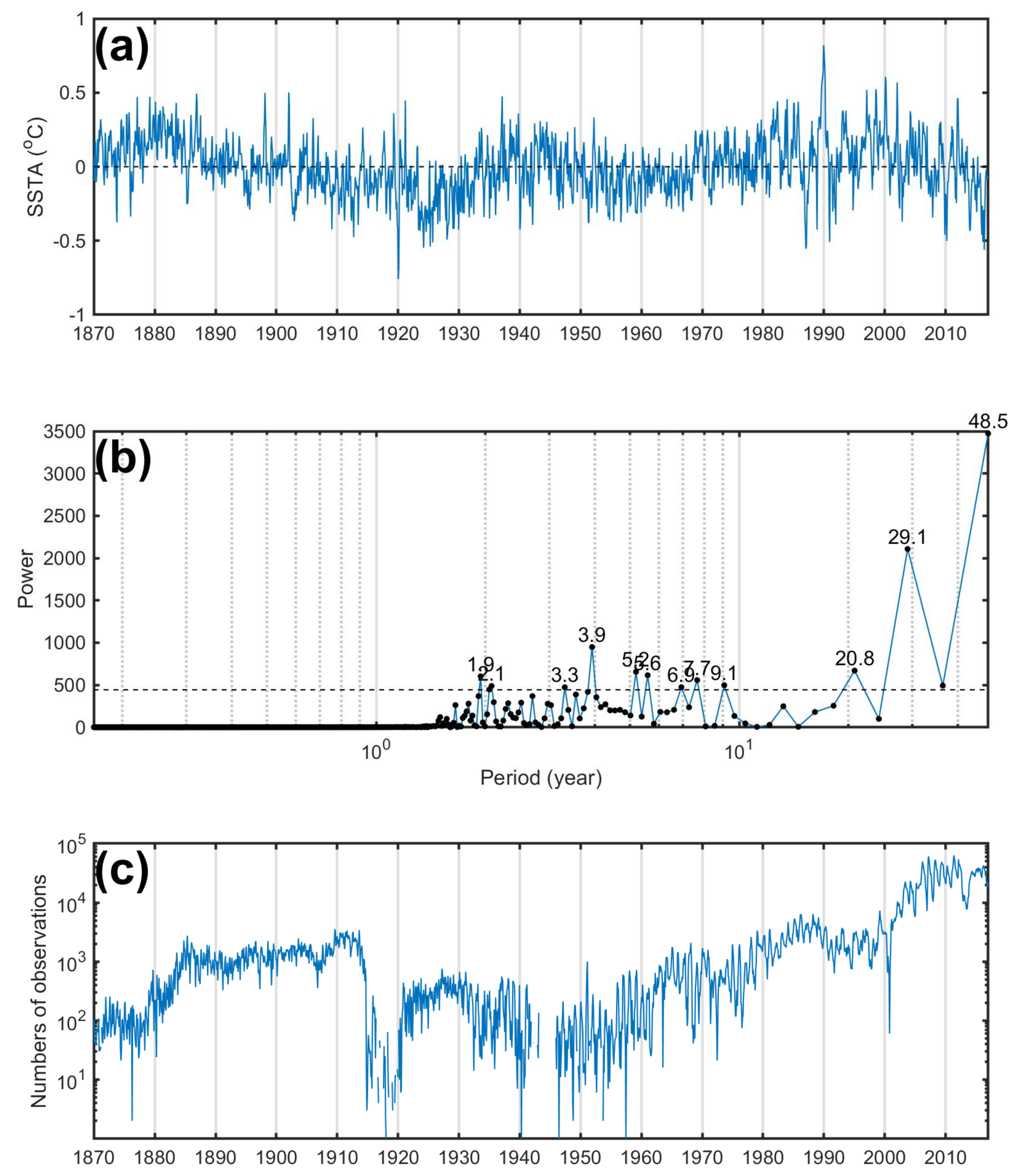
Figure 2a plots the SSTA time series, showing the clear inter-annual and inter-decadal variations in our study area. The strongest cycles of the variations, as shown using the FFT, are between 2.1 and 49 years (Figure 2b). We also noticed that numbers of observations in the study area are incomplete especially during the two World Wars (1914–1918, and 1938–1945) (Figure 2c), it may result in some uncertainties in discussing findings in this study. Although the observations are not continuous, previous studies showed that the South Atlantic Ocean was found to also experience significant inter-annual to multi-decadal variabilities in hydrology [1,27,28,29,30]. Interestingly, the results of the FFT analysis indicate a significant spectral peak at the cycles of 2–5 years, which matches the 3–5-year cycles of ENSO in recent decades [31]. In fact, the inter-annual SST variability in the South Atlantic Ocean was suggested to have a certain correlation to the variabilities in the climate in South America [17,31]. Such results suggest that changes in the SSTA in the South Atlantic Ocean could be similar to those in the tropic and subtopic Pacific Ocean. To investigate this relationship, we examine the correlations between the variations of SSTA in our study area and the ENSO as follows.
3.2. Relationships between the SSTA Composites and the ENSO
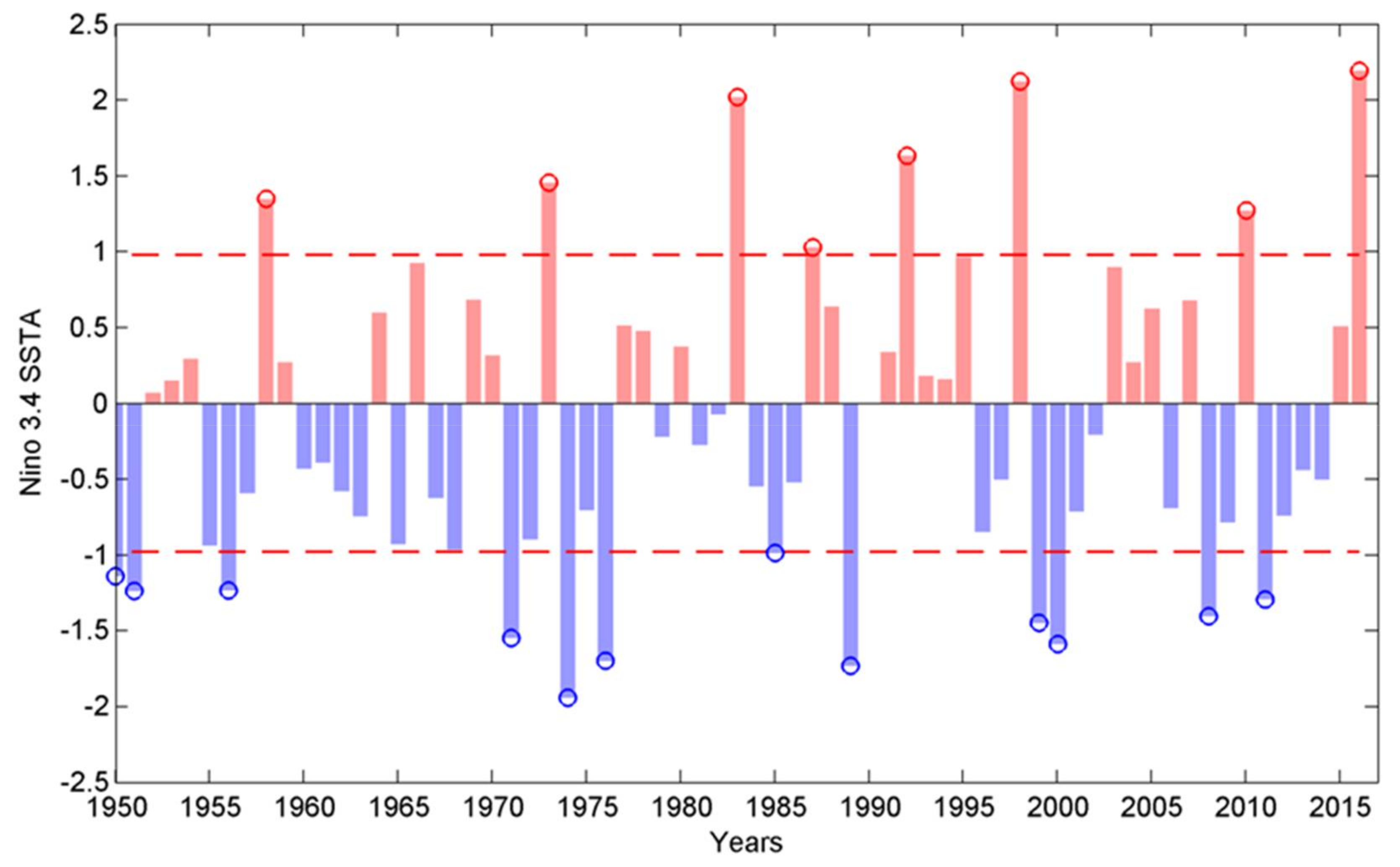
It is noteworthy that the variations in the SSTA shown in Figure 2 might correlate with the ENSO phenomena. To simplify, we first adopt the definition and methodology from KaoandYu [32] and hence identify the ENSO years using the following method. The years of the ENSO years/events are identified when the December–February means of the Niño 3.4 SSTA depart from zero by more than one standard deviation of 0.98 °C (Figure 3). Table 1 lists the years of ENSO events between 1950 and 2016.
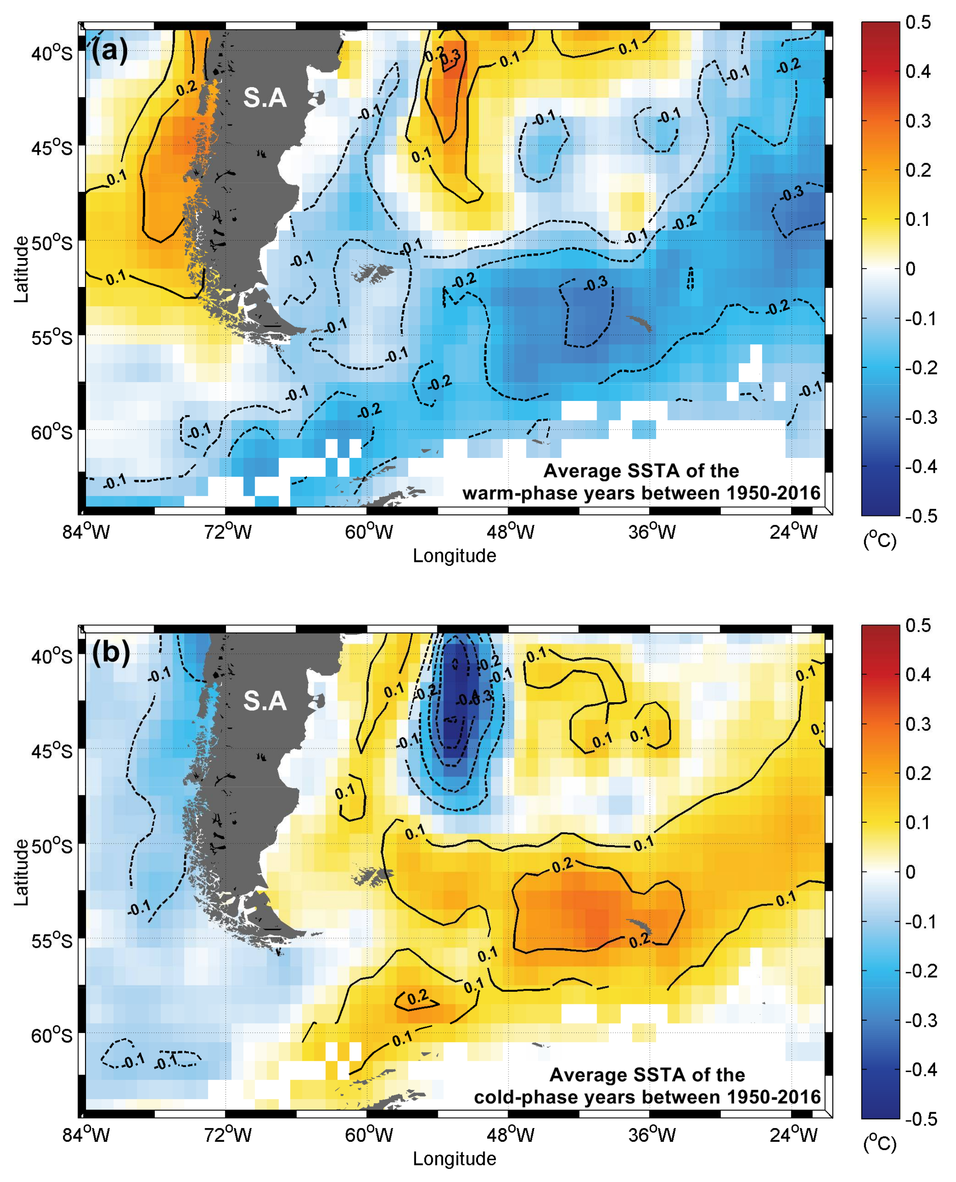
Figure 4 shows the spatial distributions of the SSTA composites during the ENSO warm- or cold-phase years between 1950 and 2016. The results show that, in the warm-phase years, the vicinity of Peru and the BMC region showed positive SSTAs (Figure 4a). Meanwhile, the South and Southwest Atlantic Ocean showed negative SSTAs. In contrast, in the cold-phase years, the vicinity of Peru and the BMC region showed negative SSTAs (Figure 4b). Meanwhile, the Southwest Atlantic Ocean showed positive SSTAs. Such a result shows that the SSTA variability in our study area is highly correlated with that of the Niño 3.4 region and is regionally dependent. In a nutshell, the variability of the SSTAs in the vicinity of Peru and the BMC region was in phase with that of the Niño 3.4 SSTA, while the variability of the SSTAs in the South and Southeast Atlantic Ocean was out of phase with that of the Niño 3.4 SSTA.
3.3. The Evolution of the SST Anomalies Associated with ENSO-Related Phenomena
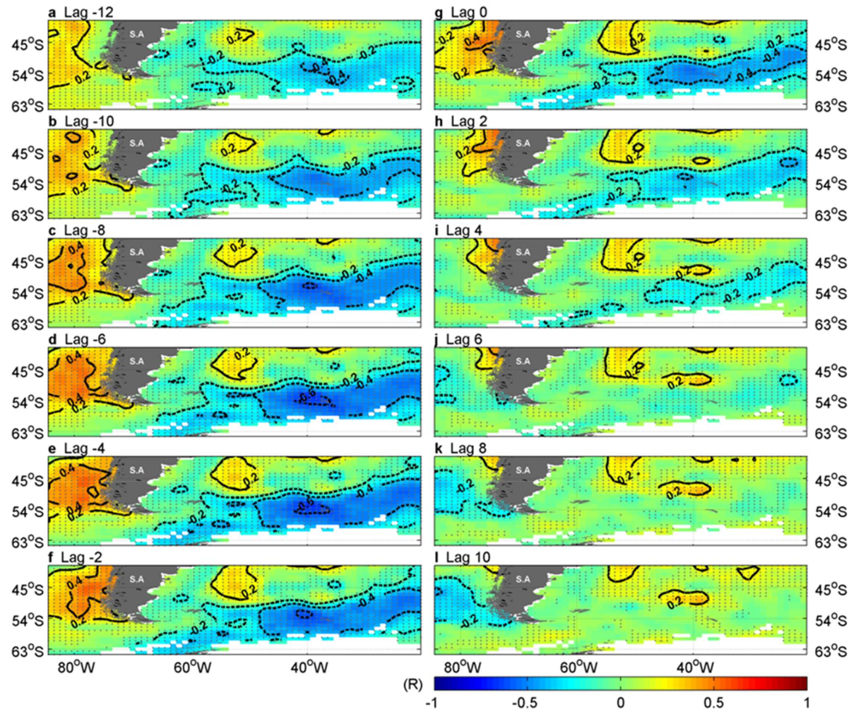
Previous studies have shown that regions experiencing the influences of ENSO on SST or seawater chemistry had different time phase differences in their temporal changes [33,34]. The changes in SSTAs in our study area might temporally lead or lag that of the Niño 3.4 SSTA. To examine this relationship, the cross-correlation coefficient (R) between the SSTAs in our study area and the Niño 3.4 SSTA with different lagging phase was determined. Figure 5 shows the spatial distributions of the R values.
Our results show that the R values reached a maximum of 0.56 for the Southeast Pacific Ocean and a minimum −0.67 for the Southeast Atlantic Ocean with the SSTAs leading the Niño 3.4 SSTA by four months (Table 2, Figure 5). Notably, the magnitudes of the R values decreased when the SSTAs lagged behind the Niño 3.4 SSTA (e.g., lagging the Niño 3.4 SSTA by two to 12 months, Figure 5). The SSTAs leading the ENSO may be due to background oceanic circulation that allows the warming signal to propagate northward via the Peru Current during the development of ENSO [35]. By contrast, the ENSO could lead the changes of regional climate in the Asian and the Antarctic [36,37].
It is worth mentioning that the spatial distributions of the average SSTA shown in Figure 5 as well as the R values shown in Figure 5 are regionally dependent events. It is likely that, during the warm phases of ENSO, the Peru Current originated by the north flow of ACC decreased, and vice versa in the cold phases. The decrease in the amount of incoming relatively cold ACC causes an increase in the SST, and vice versa. Therefore, the SSTAs in the Southeast Pacific Ocean showed positive values in the warm phases and negative values in the cold phases. In contrast, the eastward flow of the ACC enhanced during the ENSO warm phases, and vice versa in the cold phases. Therefore, the SSTAs in the Southeast Atlantic Ocean showed negative values in the warm phases and positive values in the cold phases. Although the driving forces for the changes remain unclear, it is clear that the SSTAs in our study area have patterns of changes similar to those of the Niño 3.4 SSTA. The implication is that a change in the strength of the ENSO, the circulation in our study area, or a combination of both under a changing climate could change the climate in oceans in higher latitudes. On the one hand, ENSO could influence the SSTAs in the regions of Southeast South America and Southeast Atlantic Ocean due to the teleconnection between the tropical Pacific and the Southern Ocean via the Rossby wave train [35,38]. On the other hand, the warming signal in the study area could propagate northward via the Peru Current to further enhance ENSO phenomena [35].
4. Conclusions
Using a 147-year dataset from the Met Office Hadley Centre, we show that the SSTA in the oceans west and east of South America and the Antarctic Peninsula have strong positive and negative correlations with the Niño 3.4 SSTA, respectively. Likely, the changes are due to the changes in the circulation of the ACC. Statistically, the temporal variations in the SSTA of the ACC lead the Niño 3.4 SSTA by four to six months. Although the driving force is unclear, our study implies that changes in the strength of ENSO or circulation of the ACC under changing climate may change the climate in higher-latitude oceans.
Author Contributions
C.-P.L. designed the study. Y.-C.H. analyzed the data and led the writing. C.-P.L., C.-R.W., Y.-L.W., and H.-K.L. contributed to the writing and data interpretation. Contextualization: C.-R.W.
Acknowledgments
The authors would like to thank Met Office Hadley Centre and NOAA for providing the invaluable data. We thank three anonymous reviewers’ constructive comments which clarify and strengthen the manuscript. This research was supported by the Ministry of Science and Technology, ROC, under grants MOST 104-2611-M-003-002-MY3.
Conflicts of Interest
The authors declare no conflict of interest.
References
- Olbers, D.; Borowski, D.; Völker, C.; Wolff, J.O. The dynamical balance, transport and circulation of the Antarctic Circumpolar Current. Antarct. Sci. 2004, 16, 439–470. [Google Scholar] [CrossRef] [Green Version]
- Sloyan, B.M.; Rintoul, S.R. The Southern Ocean Limb of the Global Deep Overturning Circulation. J. Phys. Oceanogr. 2001, 31, 143–173. [Google Scholar] [CrossRef]
- Sloyan, B.M.; Rintoul, S.R. Circulation, Renewal, and Modification of Antarctic Mode and Intermediate Water. J. Phys. Oceanogr. 2001, 31, 1005–1030. [Google Scholar] [CrossRef]
- Swart, S.; Speich, S. An altimetry-based gravest empirical mode south of Africa: 2. Dynamic nature of the Antarctic Circumpolar Current fronts. J. Geophys. Res. Oceans 2010, 115. [Google Scholar] [CrossRef]
- Swart, S.; Speich, S.; Ansorge, I.J.; Lutjeharms, J.R.E. An altimetry-based gravest empirical mode south of Africa: 1. Development and validation. J. Geophys. Res. Oceans 2010, 115. [Google Scholar] [CrossRef]
- Billany, W.; Swart, S.; Hermes, J.; Reason, C.J.C. Variability of the Southern Ocean fronts at the Greenwich Meridian. J. Mar. Syst. 2010, 82, 304–310. [Google Scholar] [CrossRef]
- Peterson, R.G. The boundary currents in the western Argentine Basin. Deep Sea Res. Part A Oceanogr. Res. Pap. 1992, 39, 623–644. [Google Scholar] [CrossRef]
- Rivas, A.L. Spatial and temporal variability of satellite-derived sea surface temperature in the southwestern Atlantic Ocean. Cont. Shelf Res. 2010, 30, 752–760. [Google Scholar] [CrossRef]
- Piola, A.R.; Gordon, A.L. Intermediate waters in the southwest South Atlantic. Deep Sea Res. Part A. Oceanogr. Res. Pap. 1989, 36, 1–16. [Google Scholar] [CrossRef]
- Piola, A.; Matano, R. Brazil and Falklands (Malvinas) currents. Ocean Curr. Deriv. Encycl. Ocean Sci. 2001, 1, 340–349. [Google Scholar]
- Chelton, D.B.; Schlax, M.G.; Witter, D.L.; Richman, J.G. Geosat altimeter observations of the surface circulation of the Southern Ocean. J. Geophys. Res. Oceans 1990, 95, 17877–17903. [Google Scholar] [CrossRef]
- Giannini, A.; Kushnir, Y.; Cane, M.A. Interannual Variability of Caribbean Rainfall, ENSO, and the Atlantic Ocean. J. Clim. 2000, 13, 297–311. [Google Scholar] [CrossRef]
- Montecinos, A.; Díaz, A.; Aceituno, P. Seasonal Diagnostic and Predictability of Rainfall in Subtropical South America Based on Tropical Pacific SST. J. Clim. 2000, 13, 746–758. [Google Scholar] [CrossRef]
- Souza, E.B.D.; Kayano, M.T.; Tota, J.; Pezzi, L.; Fisch, G.; Nobre, C. On the influences of the El Niño, La niña and Atlantic Dipole Paterni on the Amazonian Rainfall during 1960–1998. Acta Amazon. 2000, 30, 305–318. [Google Scholar] [CrossRef]
- Cazes-Boezio, G.; Robertson, A.W.; Mechoso, C.R. Seasonal Dependence of ENSO Teleconnections over South America and Relationships with Precipitation in Uruguay. J. Clim. 2003, 16, 1159–1176. [Google Scholar] [CrossRef]
- Andreoli, R.V.; Kayano, M.T. ENSO-related rainfall anomalies in South America and associated circulation features during warm and cold Pacific decadal oscillation regimes. Int. J. Climatol. 2005, 25, 2017–2030. [Google Scholar] [CrossRef]
- Andreoli, R.V.; Kayano, M.T. Tropical Pacific and South Atlantic effects on rainfall variability over Northeast Brazil. Int. J. Climatol. 2006, 26, 1895–1912. [Google Scholar] [CrossRef]
- Kayano, M.T.; Andreoli, R.V.; Souza, R.A.F.D. Relations between ENSO and the South Atlantic SST modes and their effects on the South American rainfall. Int. J. Climatol. 2013, 33, 2008–2023. [Google Scholar] [CrossRef]
- Tedeschi, R.G.; Collins, M. The influence of ENSO on South American precipitation during austral summer and autumn in observations and models. Int. J. Climatol. 2016, 36, 618–635. [Google Scholar] [CrossRef]
- Jacques-Coper, M.; Brönnimann, S. Summer temperature in the eastern part of southern South America: Its variability in the twentieth century and a teleconnection with Oceania. Clim. Dyn. 2014, 43, 2111–2130. [Google Scholar] [CrossRef]
- Kayano, M.T.; Andreoli, R.V.; Souza, R.A.F.D.; Garcia, S.R. Spatiotemporal variability modes of surface air temperature in South America during the 1951–2010 period: ENSO and non-ENSO components. Int. J. Climatol. 2017, 37, 1–13. [Google Scholar] [CrossRef]
- Scardilli, A.S.; Llano, M.P.; Vargas, W.M. Temporal analysis of precipitation and rain spells in Argentinian centenary reference stations. Theor. Appl. Climatol. 2017, 127, 339–360. [Google Scholar] [CrossRef]
- Wang, C.; Xie, S.P.; Carton, J.A. A global survey of ocean–atmosphere interaction and climate variability. Earth’s Clim. 2004, 1–19. [Google Scholar] [CrossRef]
- Rayner, N.; Parker, D.E.; Horton, E.; Folland, C.; Alexander, L.; Rowell, D.; Kent, E.; Kaplan, A. Global analyses of sea surface temperature, sea ice, and night marine air temperature since the late nineteenth century. J. Geophys. Res. Atmos. 2003, 108. [Google Scholar] [CrossRef] [Green Version]
- Trenberth, K.E. The Definition of El Niño. Bull. Am. Meteorol. Soc. 1997, 78, 2771–2778. [Google Scholar] [CrossRef]
- Lentini, C.A.D.; Campos, E.J.D.; Podestá, G.G. The annual cycle of satellite derived sea surface temperature on the western South Atlantic shelf. Revista Brasileira de Oceanografia 2000, 48, 93–105. [Google Scholar] [CrossRef]
- Venegas, S.A.; Mysak, L.A.; Straub, D.N. An interdecadal climate cycle in the South Atlantic and its links to other ocean basins. J. Geophys. Res. Oceans 1998, 103, 24723–24736. [Google Scholar] [CrossRef]
- Reason, C.J.C. Multidecadal climate variability in the subtropics/mid-latitudes of the Southern Hemisphere oceans. Tellus A 2000, 52, 203–223. [Google Scholar] [CrossRef]
- Palastanga, V.; Vera, C.; Piola, R.A. On the leading modes of sea surface temperature variability in the South Atlantic Ocean. Clivar Exch. 2002, 7, 12–15. [Google Scholar]
- Reason, C.J.C.; Rouault, M.; Melice, J.-L.; Jagadheesha, D. Interannual winter rainfall variability in SW South Africa and large scale ocean–atmosphere interactions. Meteorol. Atmos. Phys. 2002, 80, 19–29. [Google Scholar] [CrossRef]
- Peterson, R.G.; White, W.B. Slow oceanic teleconnections linking the Antarctic Circumpolar Wave with the tropical El Niño-Southern Oscillation. J. Geophys. Res. Oceans 1998, 103, 24573–24583. [Google Scholar] [CrossRef]
- Kao, H.-Y.; Yu, J.-Y. Contrasting Eastern-Pacific and Central-Pacific Types of ENSO. J. Clim. 2009, 22, 615–632. [Google Scholar] [CrossRef]
- Wu, C.-R. Interannual modulation of the Pacific Decadal Oscillation (PDO) on the low-latitude western North Pacific. Prog. Oceanogr. 2013, 110, 49–58. [Google Scholar] [CrossRef]
- Huang, T.-H.; Chen, C.-T.A.; Zhang, W.-Z.; Zhuang, X.-F. Varying intensity of Kuroshio intrusion into Southeast Taiwan Strait during ENSO events. Cont. Shelf Res. 2015, 103, 79–87. [Google Scholar] [CrossRef]
- John, T. The El Niño–southern oscillation and Antarctica. Int. J. Climatol. 2004, 24, 1–31. [Google Scholar] [CrossRef]
- Kawamura, R.; Suppiah, R.; Collier, M.A.; Gordon, H.B. Lagged relationships between ENSO and the Asian Summer Monsoon in the CSIRO coupled model. Geophys. Res. Lett. 2004, 31. [Google Scholar] [CrossRef]
- Ledley, T.S.; Huang, Z. A possible ENSO signal in the Ross Sea. Geophys. Res. Lett. 1997, 24, 3253–3256. [Google Scholar] [CrossRef]
- Karoly, D.J. Southern Hemisphere Circulation Features Associated with El Niño-Southern Oscillation Events. J. Clim. 1989, 2, 1239–1252. [Google Scholar] [CrossRef]
Figure 1.
Topography and schematic sketches of the Antarctic Circumpolar Current (ACC), Peru Current, Falkland Current and Brazil Current (yellow arrows) in the study area. The research area indicated by the red rectangular box is between 38.5° S–64.5° S and 84.5° W–20.5° W.
Figure 1.
Topography and schematic sketches of the Antarctic Circumpolar Current (ACC), Peru Current, Falkland Current and Brazil Current (yellow arrows) in the study area. The research area indicated by the red rectangular box is between 38.5° S–64.5° S and 84.5° W–20.5° W.

Figure 2.
The (a) Sea surface temperature anomaly (SSTA) time series in the study area (38.5° S–64.5° S and 84.5° W–20.5° W) between 1870 and 2016, and the (b) power computed by the Fast Fourier Transform (FFT) method. The values show the periods (year) with the highest power which statistical significance above 99% confidence level (dash line). (c) Numbers of observations in the study area.

Figure 3.
Time series of December–February means of the Niño 3.4 SSTA. The dashed red lines show one standard deviation of ±0.98 °C. The bars with open cycles indicate the El Niño-Southern Oscillation (ENSO) years.
Figure 3.
Time series of December–February means of the Niño 3.4 SSTA. The dashed red lines show one standard deviation of ±0.98 °C. The bars with open cycles indicate the El Niño-Southern Oscillation (ENSO) years.

Figure 4.
The spatial distribution of the average SSTA in the (a) warm-phase (larger than 1 standard deviation) and (b) cold-phase (less than −1 standard deviation) years of ENSO (listed in Table 1 and shown in Figure 4) between 1950 and 2016. The ocean areas with incomplete data are shown in white.

Figure 5.
Distributions of R values with different lagging phases between the SSTA and the Niño 3.4 SSTA. Positive lags denote that the Niño 3.4 SSTA leads the SSTA in the study area. Dots indicate statistical significance above 99% confidence level.
Figure 5.
Distributions of R values with different lagging phases between the SSTA and the Niño 3.4 SSTA. Positive lags denote that the Niño 3.4 SSTA leads the SSTA in the study area. Dots indicate statistical significance above 99% confidence level.


Table 1.
List of the ENSO years between 1950 and 2016 (see Figure 3).
Table 1.
List of the ENSO years between 1950 and 2016 (see Figure 3).
| Year | |
|---|---|
| >1 std (warm phase year) | 1957–1958, 1972–1973, 1982–1983, 1986–1987, 1991–1992, 1997–1998, 2009–2010, 2015–2016 |
| <−1 std (cold phase year) | 1950–1951, 1951–1952, 1955–1956, 1970–1971, 1973–1974, 1975–1976, 1984–1985,1988–1989,1998–1999, 1999–2000, 2007–2008, 2010–2011 |
Table 2.
The maximum and minimum R values of each panel in Figure 5.
Table 2.
The maximum and minimum R values of each panel in Figure 5.
| No. of Month That SSTA Lagged the Niño 3.4 SSTA | R Value | |
|---|---|---|
| Max | Min | |
| −12 | 0.386 | −0.465 |
| −10 | 0.436 | −0.542 |
| −8 | 0.476 | −0.614 |
| −6 | 0.539 | −0.658 |
| −4 | 0.558 | −0.665 |
| −2 | 0.541 | −0.622 |
| 0 | 0.507 | −0.532 |
| 2 | 0.511 | −0.434 |
| 4 | 0.485 | −0.344 |
| 6 | 0.425 | −0.305 |
| 8 | 0.384 | −0.390 |
| 10 | 0.381 | −0.429 |
| 12 | 0.346 | −0.419 |
© 2018 by the authors. Licensee MDPI, Basel, Switzerland. This article is an open access article distributed under the terms and conditions of the Creative Commons Attribution (CC BY) license (http://creativecommons.org/licenses/by/4.0/).
Share and Cite
MDPI and ACS Style
Hsu, Y.-C.; Lee, C.-P.; Wang, Y.-L.; Wu, C.-R.; Lui, H.-K. Leading El-Niño SST Oscillations around the Southern South American Continent. Sustainability 2018, 10, 1783. https://doi.org/10.3390/su10061783
AMA Style
Hsu Y-C, Lee C-P, Wang Y-L, Wu C-R, Lui H-K. Leading El-Niño SST Oscillations around the Southern South American Continent. Sustainability. 2018; 10(6):1783. https://doi.org/10.3390/su10061783
Chicago/Turabian StyleHsu, Yu-Chen, Chung-Pan Lee, You-Lin Wang, Chau-Ron Wu, and Hon-Kit Lui. 2018. "Leading El-Niño SST Oscillations around the Southern South American Continent" Sustainability 10, no. 6: 1783. https://doi.org/10.3390/su10061783
Note that from the first issue of 2016, this journal uses article numbers instead of page numbers. See further details here.