Revisiting the Solid Flux Theory

Abstract

Several variations of the basic activated sludge process and of the related design procedures for final clarifiers have been developed, which are frequently based on the well-known solid flux theory (SFT). In this paper, by using the Lambert W function and a “virtual” solid flux corresponding to the Vesilind parameters’ ratio, the SFT is reformulated, and dimensionless groups are detected, which highly reduce the number of parameters that are involved in the final clarifiers’ design procedure. The derived dimensionless relationships and the corresponding plots have general validity since they can be applied to all the possible design/verification parameter combinations. Moreover, it is shown that for any input dataset, the suitable domains of the SS concentration and of the solid flux can be simply expressed by the two branches of the Lambert W function. By using data retrieved from the literature, several numerical applications and validations of the dimensionless relationships are performed. Finally, it is shown that by introducing in the SFT a new reduction hydrodynamic factor, ρ_R, to be applied to the modified return flow formula rather than to the limiting solid flux as in the past, a significant improvement in the comparison between the results by theory and by experiments can be obtained.

1. Introduction

The importance of well-designed final clarifiers is fully acknowledged, since they determine the operating accuracy of the activated sludge (AS) process, the most used biological process in wastewater treatment plants (WWTPs) [1]. The AS process has been employed for pollutant removal for more than a century owing to its high nutrient removal and biomass retention capabilities and toxin degradation [2].

As environmental regulations become more stringent, increased pressure is placed on WWTPs to enhance their performance [3]. With the water and energy crisis occurring in our lifetime, various reports have identified that methods of addressing, assessing, and reducing energy must be explored [4]. The AS process requires energy to transfer the sludge back to the aeration tank and power the aerators; thus, they need to be properly designed.

The activated sludge wastewater treatment process is based on a multi-chamber reactor unit, which uses microorganisms as a method to remove nutrients from the water and uses oxygen to establish and regulate aerobic conditions and to suspend the sludge. Following the aeration step, the microorganisms need to be separated from the liquid by sedimentation; thus, a final clarification is necessary. A portion of the biological sludge extracted by the bottom of the final clarifier is recycled to the aeration tank to maintain appropriate levels of biomass concentration in the dispersed-growth reactor. The remainder (excess sludge) is removed from the process and sent for sludge processing to maintain in the system an almost constant biomass concentration [5]. The appropriate design of the final clarifiers is compulsory to assure the quality of the treated effluent according to its suspended solids (SS) concentration.

Compared to other types of wastewater treatment, activated sludge WWTPs have several benefits that explain why the activated sludge (AS) process has been widely applied, investigated, and interpreted [2,5,6,7,8,9].

Recently, Jasim [10] used the GPS-X model, which is the first commercially released dynamic wastewater treatment plant simulator, for the mathematical modeling, control, optimization, and management of wastewater treatment plants while designing the Al-Hay city WWTP in the south of Baghdad, Iraq.

Islam et al. [11] suggested a design procedure of an activated sludge WWTP consisting of an activated sludge reactor and settling tank that includes the growth kinetics of microorganisms, causing the degradation of biodegradable pollutants, and assuming that the settling characteristics are fully described by a power law. Moreover, Islam et al. [11] developed a procedure to calculate the activated sludge concentration corresponding to an optimal condition, for which the total required area of the plant is minimum, for a given microbiological system and return ratio.

By applying Vitasovic’s solid flux model [12] to the sewage plant of Siegen (Germany), Koehne et al. [13] investigated the complex dynamic process of clarification, settling, and thickening in final clarifiers of wastewater treatment plants, which are very sensitive to changes in hydraulic and organic loading, and compared the underflow and effluent suspended solids concentrations with simulation results.

By using the method of radioisotope tracer, Kim et al. [14] made a detailed comparison of the calculated residence time distribution curves, with measurements performed inside the clarifier as well as the exhaust, and predicted the characteristics of clarifier flow, such as the waterfall phenomenon at the front end of the clarifier, the bottom density current in the settling zone, and the upward flow in the withdrawal zone.

Several variations of the basic activated sludge process, such as extended aeration and oxidation ditches, are in common use, but the basic principles are almost similar. Most of the commonly applied models are based on the sedimentation theory first suggested by Kynch [15], according to the solids flux theory (SFT). A shortcoming of using SFT is that it does not produce an explicit equation for the representation of limiting solids flux [16]. As a result, many researchers suggested SFT graphical solutions [17,18,19,20,21].

Diehl [22] stated that the SFT can be described conveniently within a larger theory of nonlinear partial differential equations (PDEs) [23] with discontinuous coefficients which has evolved since the 1990s. Diehl [22] showed that concepts such as state point, limiting solid flux, optimal operation, sludge blanket level, and thickening and clarification failure can be identified naturally within a first-order PDE model of the clarification–thickening process.

Contrarily to PDE models, it should be noted that the usefulness of simplified analytical solutions [24], such as those found in many other contexts [25,26], helps the insight into the problem prior to the application of time-consuming numerical methods. On the latter is focused this paper, which recalls the common SFT in order to obtain further design simplification. Thus, a reformulated SFT theory is developed in this work, allowing to design activated sludge final clarifiers according to a general design procedure that can be applied for any input dataset, which seems to be not available.

The objective of this paper is to revisit the theory of solid flux, consolidating the high number of design variables in a much smaller number of dimensionless groups. To this end, the Lambert W function was introduced, which suggested that the key parameter is the normalized limiting suspended solids (SS) concentration, which is related to the other design parameters, thus simplifying and generalizing a lot the design procedure of the final clarifier. Moreover, for verification purposes, it is shown that the behavior of different operating scenarios can be predicted easily, which could be useful for the management stage. Using the detected dimensionless groups, different applications are performed and discussed. Finally, some of the dimensionless relationships are compared with experimental data from other researchers.

The paper is organized as follows. Following this introduction, in Section 2, the common SFT is briefly summarized with no novelty, but it helps in understanding the new derivations. In Section 2.1, Section 2.2, Section 2.3, Section 2.4 and Section 2.5, the Lambert W function, a “virtual” solid flux corresponding to the Vesilind parameters’ ratio, and the dimensionless groups are introduced; the effect of the operating conditions on SS loading variability is focused on; and simple relationships of the domains of the SS concentration and of the solid flux are derived. In Section 3, a numerical application of the dimensionless relationships is performed, while in Section 4, the derived relationships are validated by using experimental data, and a new reduction hydrodynamic factor, ρ_R, is introduced. The paper is concluded in Section 5.

2. Theory

Under a steady state, the limiting solids flux, G_L (kg m⁻² h⁻¹), is commonly evaluated according to the well-known solids flux theory [15], as applied by many researchers [22,27,28,29]. The total solids flux to the final clarifier, G (kg m⁻² h⁻¹), is given by the following:

$$G=G_v+G_u=v x+u x$$

(1)

where G_v (kg m⁻² h⁻¹) and G_u (kg m⁻² h⁻¹) are the solids flux contributions due to gravity and the activated sludge extraction (underflow flux), respectively, which in turn depend on the zone-settling velocity of the activated sludge v (m h⁻¹) and on the recycle velocity, u (m h⁻¹), respectively, and on the suspended solids (SS) concentration, x (kg m⁻³), also denoted as biomass concentration.

According to Vesilind [30], who first proposed the relationship among zone-settling velocity, solids concentration, and sludge settleability, the settling velocity, v, can be expressed by the exponential low well [30]:

$$v=v_0 {\mathrm{e}}^{-k x}$$

(2)

where v₀ (m h⁻¹) and k (m³ kg⁻¹) are empirical coefficients expressing the settling velocity under zero suspended solids concentration (scale factor) and the exponential decay constant (shape factor), respectively.

It should be noted that other models were also applied in the literature [11,23,31,32,33]. However, the Vesilind model, which is considered in this work, is the most used since it works well in most cases [34,35,36], thus making the following derivations widely applicable.

Substituting Equation (2) into Equation (1) yields the following:

$$G=x v_0 {\mathrm{e}}^{-k x}+x u$$

(3)

Determining the limiting solids flux, G_L (kg m⁻² h⁻¹), requires putting the first derivative of Equation (3) with respect to x equal to zero:

$$\frac{\partial G}{\partial x}=u+v_0{ \mathrm{e}}^{-k x} \left(1-k x\right)=0$$

(4)

which provides the u relationship:

$$u=v_0{ \mathrm{e}}^{-k x_L} \left(k x_L-1\right)$$

(5)

Equation (5) can also be solved with respect to the SS concentration corresponding to the limiting condition, x_L (kg m⁻³):

$$x_L=\frac{1}{k}\left(1+\frac{u}{v_0{\mathrm{e}}^{-k x_L}}\right)$$

(6)

which is in an implicit form with respect to x_L. Contrarily to what will be shown here, x_L has usually been obtained numerically [17], as observed in Section 1. The G value corresponding to limiting solids flux, G_L, is obtained by imposing x = x_L into Equation (1):

$$G_L=x_L\left( v_0 {\mathrm{e}}^{-k x_L}+u\right)$$

(7)

By using Equation (5), G_L can also be expressed as follows:

$$G_L=v_0 k x_L^2{e}^{-k x_L}$$

(8)

Dividing G_L by u (m h⁻¹) provides the SS concentration of the recycle flow rate, x_r (kg m⁻³):

$$x_r=\frac{G_L}{u}$$

(9)

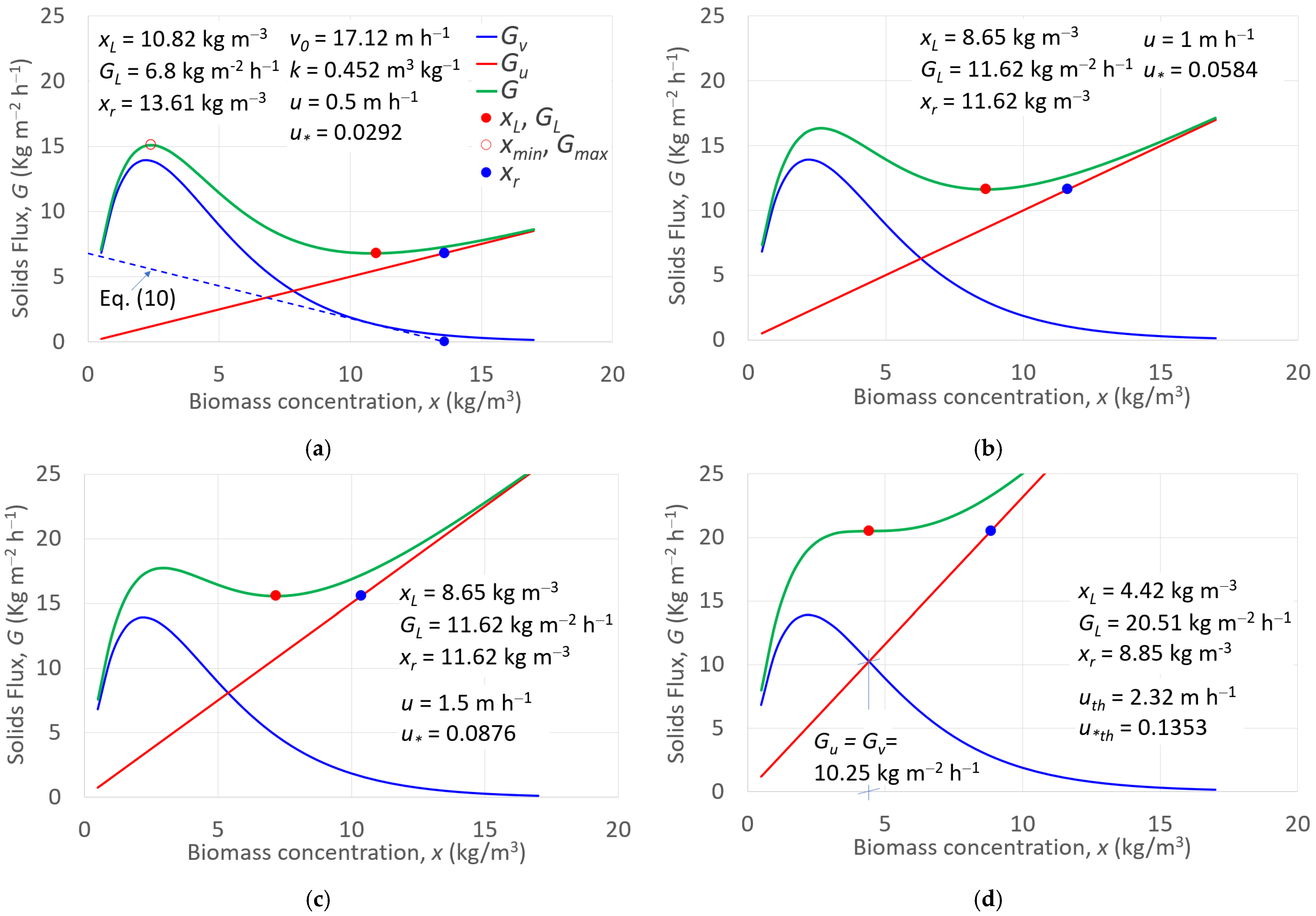
For example, for Vesilind parameters v₀ = 17.12 m h⁻¹ and k = 0.452 m³ kg⁻¹, and by assuming u = 0.5 m h⁻¹, Figure 1a shows the solids flux contributions due to gravity, G_v, and due to the activated sludge extraction, G_u, and their sum G (Equation (1)), which admits the minimum G_L = 6.8 kg m⁻² h⁻¹ for x = x_L = 10.82 kg m⁻³ (Equation (6)). The corresponding SS concentration of the recycle flow rate x_r, which lays on the straight-line G_L = u x_r (Equation (9)), is also indicated. The equation of the dashed straight line is as follows:

$$G=G_L-u x=G_L\left(1-\frac{x}{x_r} \right)$$

(10)

Equation (10) is tangent to the G_v curve at the point x = x_L, showing that at increasing G_L, the recycle flow rate must increase too, but the corresponding SS concentration will reduce (the sludge will be more diluted).

Figure 1a also shows the maximum solid flux G_max associated with the minimum biomass concentration x_min, which, together with x_L, delimits the biomass concentration domain (x_min ≤ x ≤ x_L), which can be analyzed by varying u, as will be shown in Section 2.5.

For the design purpose, by assuming the limiting solid flux G_L, the clarifier surface area, A (m²), is derived by the clarifier mass balance, yielding the following:

$$A=\frac{Q\left(1+R\right)x_0}{G_L}$$

(11)

where x₀ (kg m⁻³) is the influent SS concentration to the final clarifier; Q (m³ h⁻¹) and Q_r (m³ h⁻¹) are the wastewater and the recycle flow discharges, respectively; and R = Q_r/Q is the return ratio.

Equation (11) also makes it possible to introduce the hydraulic loading rate, C_y, which is useful for the design purpose, as it is known:

$$C_y=\frac{Q}{A}=\frac{G_L}{\left(1+R\right)x_0}$$

(12)

Once the well-known SFT has been briefly recalled, in the next section, the SFT is revisited by introducing the Lambert W function and the involved variables consolidated in dimensionless groups.

2.1. Introducing the Lambert W Function and Dimensionless Groups

The described well-known procedure is easy to apply for a fixed triplet of values (v₀, k, and u), although it does not allow a generalization to any input parameters (v₀, k, and u); moreover, Equation (6) is in an implicit form. To achieve the aim of generalizing the SFT, dimensionless groups can be suitably introduced. In this section, it is shown that introducing the Lambert W function helps address this issue and suggests consolidating input and output parameters in a compacted design procedure. Indeed, dimensionless groups are useful for scaling arguments; for consolidating experimental, analytical, and numerical results into a compact form; and to delimit the parameters domain of interest.

By using the branch W₋₁ of the Lambert W function, also denoted as the omega function or product logarithm, Equation (6), which is usually solved numerically [17], can also be expressed in the following form:

$$x_L=\frac{1}{k}\left[ 1-W_{-1}\left(-\mathrm{e} u_{\ast }\right)\right]$$

(13)

where u_* denotes the u value normalized with respect to v₀:

$$u_{\ast }=\frac{u}{v_0}$$

(14)

The Lambert W function is a multivalued function [37], namely with two branches of the converse relation of the function f(y) = y e^y, where y is any complex number and e^y is the exponential function, and it has been applied in different contexts [38,39]. When dealing with real numbers, as in the considered case, only the two brunches W₀ and W₋₁ can be considered, and the general equation y e^y = x can be solved for y, if x ≥ −1/e. In particular, for x > 0, y = W₀(x), and for −1/e ≤ x < 0, the two values W₀ and W₋₁ occur. In this case, imposing the condition x ≥ −1/e provides:

$$-\mathrm{e} u_{\ast }\ge -\frac{1}{\mathrm{e}}$$

(15)

meaning that the real solutions can be found under the following condition:

$$u_{\ast }\le \frac{1}{{\mathrm{e}}^2}=u_{\ast th}$$

(16)

or in dimensional terms:

$$u\le \frac{v_0}{{\mathrm{e}}^2}=u_{th}$$

(17)

For different v₀ values, including v₀ = 7.4 m h⁻¹ (i.e., u_th = 1 m h⁻¹) and 17.12 m h⁻¹ (Figure 1a),

Table 1. For different v₀ values, threshold u values, u_th, and the corresponding u_*th, −e u_*th, (k x_L)_th, (G_*L)_th, (k x_r)_th, and for R_c = 1, (C_*h)_th, for which Equation (21) admits real x_L solutions.

v0 (m h−1)	uth (m h−1)	u*th	−e u*th	(k xL)th	(G*L)th	(k xr)th	(C*h)th
2.1	0.28	0.1353	−0.3679	2	0.5413	4	0.1353 (Rc = 1)
3	0.41
4	0.54
5	0.68
6	0.81
7	0.95
7.4	1.00
17.12	2.32

reports the corresponding u_th = v₀ e² values.

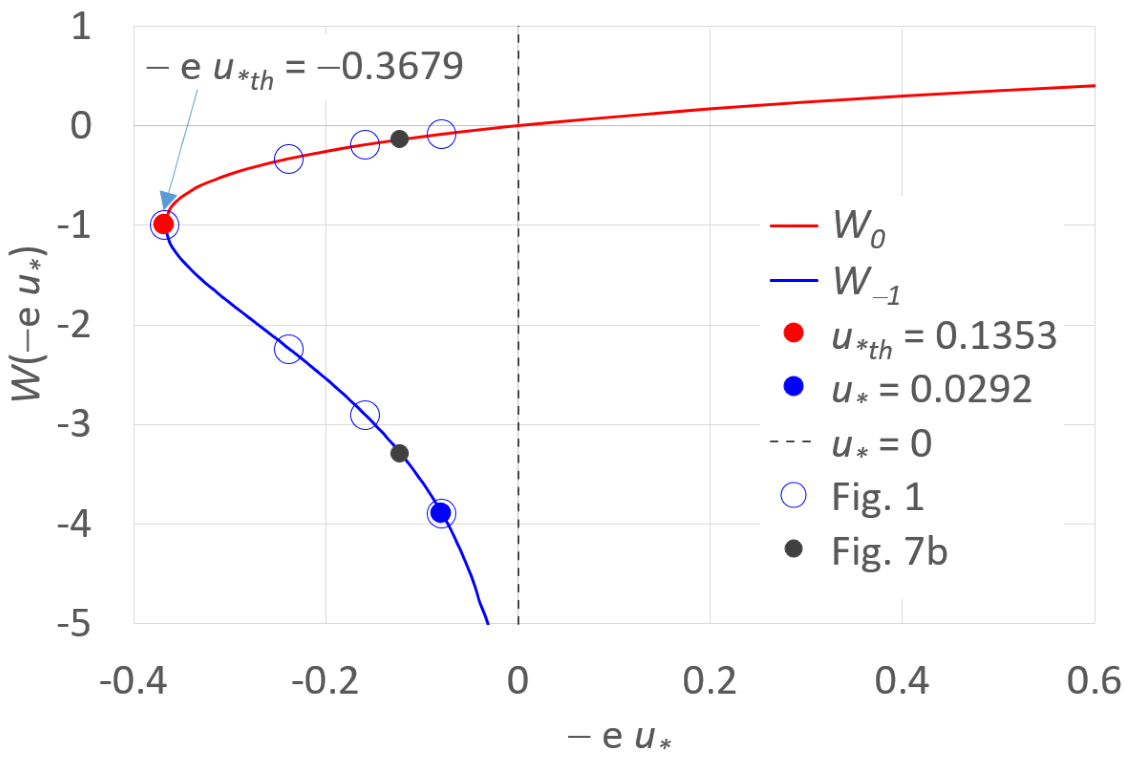
By considering the Lambert W function W(−e u_*), a graphical illustration of the u_* domain for which Equation (13) provides real solutions can be performed. Figure 2 plots the two branches of the Lambert W function, W₀ and W₋₁, versus −e u_*, together with the threshold value −e u_*th (Table 1) and the vertical dashed line that delimits the physical circumstance that u_* has to be positive (downward), depicting the x_L real solutions domain. Figure 2 also illustrates the W value corresponding to u_* = 0.0292 (−e u_* = −3.892) that refers to the application of Figure 1 and to the applications that will be performed later, which lay on the W₋₁ brunch.

The corresponding dots that lay on the W₀ brunch allow for calculating the minimum value of the biomass concentration x_min, associated with G_max (Figure 1a), if replacing W₋₁ by W₀ into Equation (13), as will be recalled in Section 2.5.

For the fixed Vesilind parameters (v₀ = 17.12 m h⁻¹ and k = 0.452 m³ kg⁻¹); for u = 1, 1.5; and for the threshold u_th = 2.32 m h⁻¹ (Table 1), for which the minimum of Equation (3) does not occur, the effect of the recycle velocity is shown in Figure 1b–d, where the solid fluxes vs. the biomass concentration are plotted.

Figure 1a–d highlight what is already known, which is recalled here only because it helps with deriving the following dimensionless derivations. In particular, at increasing u, the slope of the straight line increases, whereas the limit biomass concentration x₀ and the SS concentration of the recycle flow rate x_r decrease. For u = u_th, the minimum does not occur, but a horizontal point of inflection occurs where the curvature of the G function changes sign, thus producing a flat tangent line as the double derivate will equal to zero at its coordinates. This means that for u > u_th, x₀ itself determines the limiting concentration of the incoming biomass to the final clarifier. For u = u_th, the underflow flux achieves the solid flux contribution due to gravity (G_u = G_v, Figure 1d). The occurrence u = u_th is illustrated by the red dot in the Lambert W function (Figure 2).

The occurrence of the minimum also requires the following condition:

$$\frac{{\partial }^{2}G}{\partial x^2}=v_0 k {\mathrm{e}}^{-k x_L}\left(k x_L-2\right)>0$$

(18)

Since the factors out of brackets are positive, Equation (18) requires the following:

$$x_L>\frac{2}{k}$$

(19)

Imposing Equation (19) into Equation (5) yields the following:

$$u<v_0{ \mathrm{e}}^{-2}$$

(20)

which matches Equation (17).

Since in Equation (13) the Lambert W function is dimensionless, Equation (13) suggests that k is the scale factor of the limiting SS concentration. By consolidating the parameters k and x_L in their dimensionless product, we can write:

$$k x_L=1-W_{-1}\left(-\mathrm{e} u_{\ast }\right)$$

(21)

By denoting G₀ (kg m⁻² h⁻¹) a “virtual” solids flux corresponding to the settling velocity under zero SS concentration [40,41], we can write the following:

$$G_0=\frac{v_0}{k}$$

(22)

Normalizing G and G_L with respect to G₀ provides the dimensionless G_* and G_*L relationships, respectively:

$$G_{\ast }=\frac{G}{G_0}=k x \left({\mathrm{e}}^{-k x}+u_{\ast }\right)$$

(23)

$$G_{\ast L}=\mathsf{\rho }\frac{G_L}{G_0}=\mathsf{\rho } {\left(k x_L\right)}^2 e^{-k x_L}$$

(24)

Into Equation (24), a reduction hydrodynamic factor ρ < 1 was introduced to account for the fact that the maximum permissible solids loading of the settling tank was observed to be less than the limiting solid flux, G_L, derived by the simplified SFT [16]. This occurrence was ascribed to the hydrodynamics of the final clarifier, which behaves differently to what the simplified 1D SFT is able to describe [42].

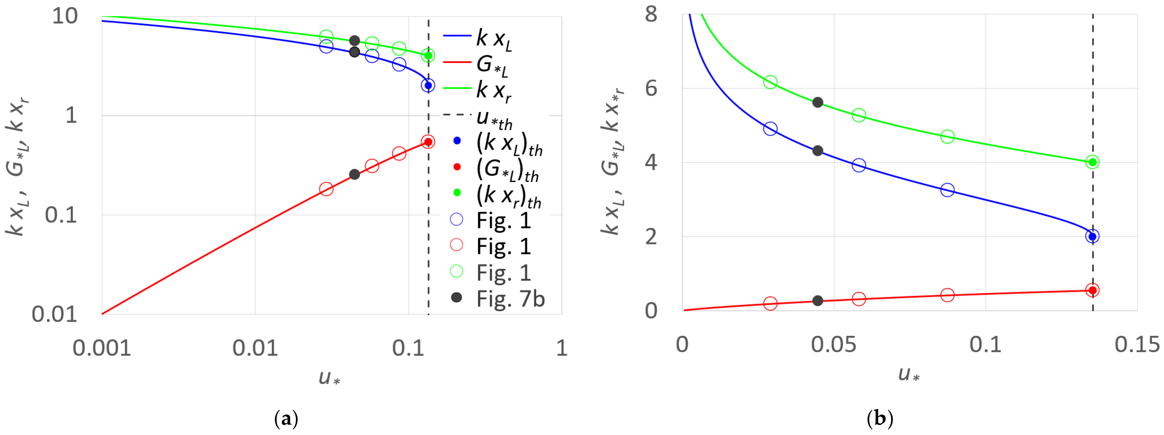
The dimensionless G_*L is plotted in Figure 3 (red lines) versus the normalized recycle velocity, u_*, in a log-log scale (Figure 3a) and in a linear scale (Figure 3b), together with the k x_L parameter (Equation (18)) versus u_*. The key parameter k x_L is useful to derive since it allows for determining any k and u_* values, the limiting SS concentration, x_L, and thus G_*L. In dimensionless terms, besides u_*, no parameters are required since they are arranged in the dimensionless groups; thus, Figure 3 covers all the possible combinations of the design parameters.

Of course, the limiting u_* condition, u_*th, does come back to k x_L as well as G_*L, which are denoted as (k x_L)_th and (G_*L)_th, respectively, as indicated in Figure 3, laying in the vertical dashed line, u_* = u_*th (Table 1). In Figure 3, the pairs (u_*, k x_L) and (u_*, G_*L) corresponding to the applications of Figure 1 are also indicated.

The dimensionless k x_L (Equation (21)) also allows for inspection of the behavior of the SS concentration of the recycle flow rate, Q_r, corresponding to the limiting condition x_r (kg m⁻³), the return rate R, and the hydraulic loading rate C_h.

For x_r, substituting Equations (5) and (8) into Equation (9) provides the following:

$$x_r=\frac{k x_L^2}{k x_L-1}$$

(25)

which can also be written in dimensionless terms as a function of k x_L as follows:

$$k x_r=\frac{{\left(k x_L\right)}^2}{k x_L-1}$$

(26)

By using Equation (21), Figure 3a,b also plot Equation (26) versus u_*, confirming the dominant role of k x_L in the final clarifier behavior.

Commonly, the influent SS concentration to the final clarifier, denoted as x₀, differs from the limiting SS concentration, x_L, and it can be shown that x₀ is related to x_L and to the return ratio, R, even by a dimensionless relationship. To show this, the mass balance needs to be invoked, as described in the next section, in dimensionless terms.

2.2. The Return Ratio by Dimensionless Groups

Under a steady state, the return ratio R can be derived by making the mass balance around the final clarifier. By assuming that the sludge blanket level in the settling tank remains constant and that the SS effluent from the final clarifier is negligible, we can write the following:

$$Q x_0=R Q\left(x_r-x_0\right)$$

(27)

where x₀ (kg m⁻³) is the influent SS concentration to the final clarifier. Substituting Equation (25) into Equation (27) yields the following:

$$R=\frac{ x_0\left(k x_L-1\right)}{k x_L^2-x_0\left(k x_L-1\right)}$$

(28)

which can be written in dimensionless terms as a function of the dimensionless k x₀ and k x_L:

$$R=\frac{k x_0\left(k x_L-1\right)}{{\left( k x_L\right)}^2-k x_0\left(k x_L-1\right)}$$

(29)

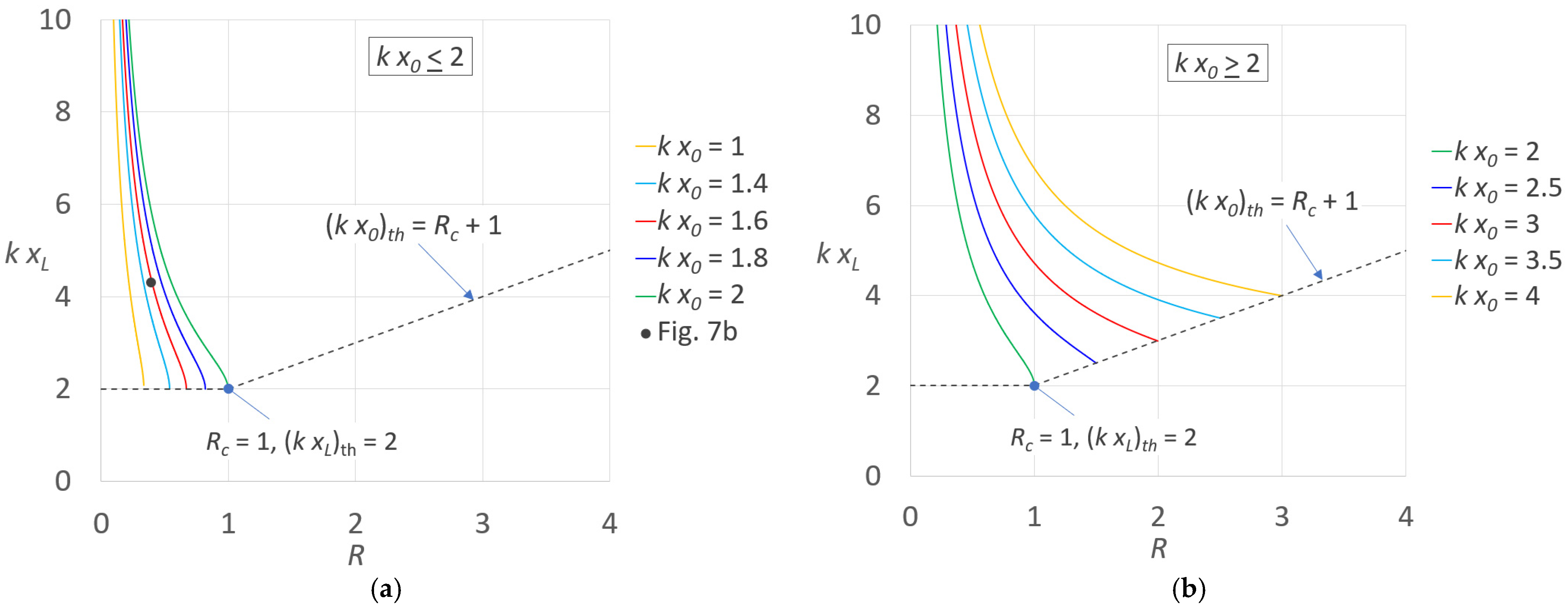
For k x₀ ≤ 2 and k x₀ ≥ 2, by varying k x_L, Equation (29) is plotted in Figure 4a and Figure 4b, respectively. The figures show that k x_L decreases at increasing R, as could be expected. For a fixed R, at increasing k x₀, k x_L increases for both k x₀ ≤ 2 and k x₀ ≥ 2, with a greater influence on the latter that could require unsuitable high R > 1 values. Contrarily, it can also be observed that for k x₀ ≤ 2, R is less than one.

In Figure 4a,b, the limiting condition is also indicated. As already discussed in Table 1, for k x₀ ≤ 2 and for any R ≤ 1, (k x_L)_th equals 2, whereas for k x₀ ≥ 2 and for R ≥ 1, since the x_L minimum does not occur, x₀ itself provides the limiting SS concentration. Therefore, imposing x_L = x₀ into Equation (29) yields the following:

$${\left(k x_0\right)}_{th}=R_c+1$$

(30)

where R_c denotes the corresponding limiting return ratio. Figure 4a also indicates the dot corresponding to the application performed later.

Of course, for u_* = u_*th, it can also be verified that substituting (k x_L)_th = 2 into Equation (30) provides R_c = 1, as indicated in Figure 4a,b. In conclusion, the following limiting conditions occur:

$${\left(k x_L\right)}_{th}=2 for R\le 1 and k x_0\le 2$$

(31)

$${\left(k x_0\right)}_{th}=R_c+1 for any R and k x_0\ge 2$$

(32)

Knowing k x_L and Equation (29) makes it possible to determine, for any R and k x₀, the limiting solid flux, G_*L, and the SS concentration of the recycle flow rate, k x_r, by using Equations (24) and (26), respectively.

The dimensionless groups detected in this section allow an SFT generalization, with reference to the limiting solid flux and the related return ratio and SS concentration to the final clarifier; however, they do not help in designing the final clarifier. To this end, in agreement with the previously introduced dimensionless groups, the normalized hydraulic loading rate needs to be defined.

2.3. Normalized Hydraulic Loading Rate

By dividing both sides of Equation (12) with respect to v₀, the dimensionless hydraulic loading rate C_*h can be expressed as:

$$C_{\ast y}=\frac{Q}{A v_0}=\frac{G_L}{\left(1+R\right)x_0{v}_0}$$

(33)

Moreover, by dividing and multiplying the right side by k, and using Equation (24), C_*h can also be rewritten as follows:

$$C_{\ast h}=\frac{Q}{A v_0}=\frac{G_{\ast L}}{\left(1+R\right) k x_0}=\frac{\mathsf{\rho } {\left(k x_L\right)}^2 e^{-k x_L}}{\left(1+R\right) k x_0}$$

(34)

again showing the important role of k x_L in C_*h. Equation (34) shows the dependence of C_*h on ρ, R, k x_L, and k x₀. The normalized influent SS concentration k x₀ can be also expressed by Equation (29):

$$k x_0=\frac{R {\left(k x_L\right)}^2}{\left(1+R\right)\left(k x_L-1\right)}$$

(35)

Substituting Equation (35) into Equation (34) provides a useful relationship of the normalized hydraulic loading rate:

$$C_{\ast h}=\frac{Q}{A v_0}=\frac{\mathsf{\rho } e^{-k x_L}\left(k x_L-1\right) }{R}$$

(36)

Equation (36) is of paramount importance for the design purpose since it describes the possible combinations of the design parameters—i.e., for any SS Vesilind parameters and influent discharge to the WWTP, Q.

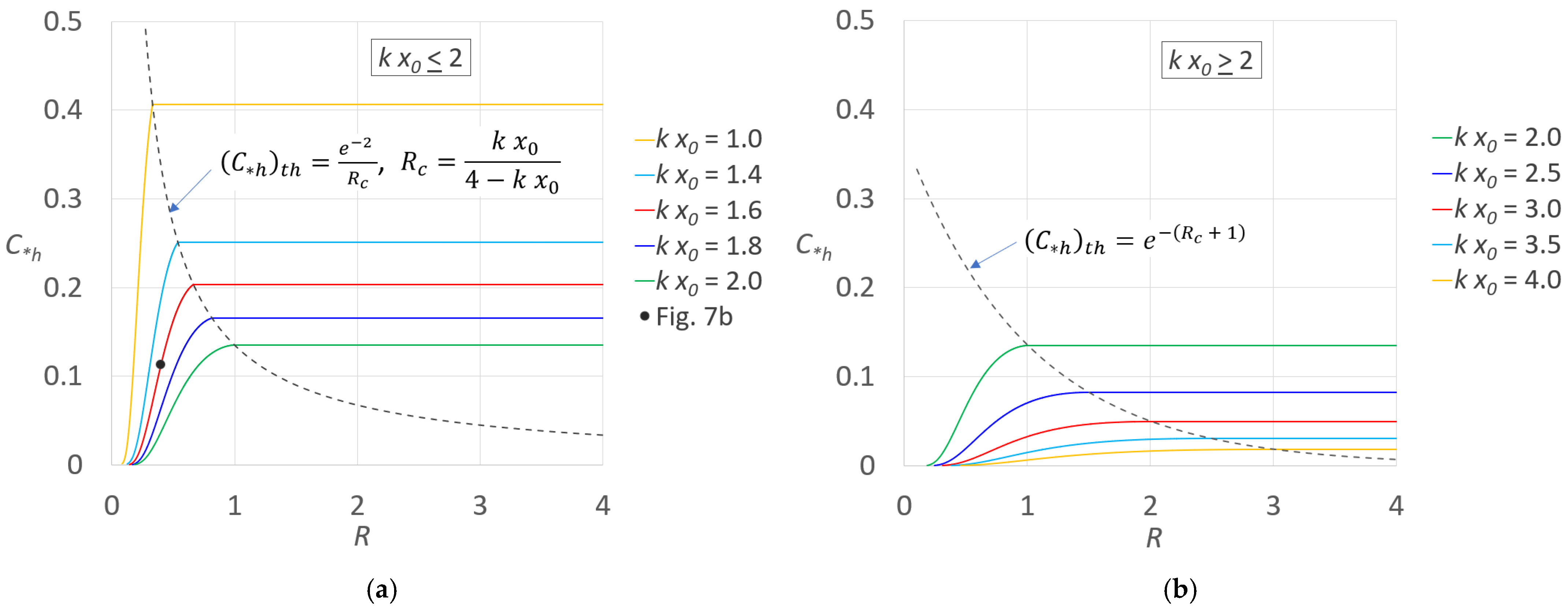
By varying k x_L, and thus R (Equation (29)), for k x₀ ≤ 2 and k x₀ ≥ 2, Equation (36) is plotted in Figure 5a and Figure 5b, respectively. The figures show that C_*h increases at increasing R, and that for a fixed R at increasing k x₀, C_*h increases for k x₀ ≤ 2 whereas it decreases for k x₀ ≥ 2.

Moreover, to k x₀ ≥ 2 correspond low C_*h values that of course make this occurrence not recommended. It can also be observed that for k x₀ ≤ 2, R is less than the unity, whereas for the not recommended condition k x₀ ≥ 2, R can also be higher than the unity.

Based on Figure 4a,b, in Figure 5a,b the limiting C_*h condition was also plotted. Similarly to k x_L, two cases can be distinguished: (i) k x₀ ≤ (k x_L)_th (R_c ≤ 1) and (ii) k x₀ ≥ (k x_L)_th (R_c ≥ 1).

For k x₀ ≤ (k x_L)_th (R_c ≤ 1), by putting k x_L = (k x_L)_th = 2 into Equation (29), the limiting condition can be written as a function of k x₀:

$$R_c=\frac{ k x_0}{4-k x_0}$$

(37)

which matches with that suggested by d’Antonio and Carbone (1987; see Equation (21)). By considering (k x_L)_th = 2 and substituting Equation (37) into Equation (36), the corresponding limiting C_*h, (C_*h)_th, can be derived (Figure 5a):

$${\left(C_{\ast h}\right)}_{th}=\frac{Q}{A v_0}=\frac{e^{-2}}{R_c}=\frac{4-k x_0 }{k x_0}{e}^{-2}$$

(38)

For k x₀ ≥ (k x_L)_th, since the x_L minimum does not occur, x₀ itself provides the limiting SS concentration, as previously observed. Putting x_L = x₀ into Equation (35), and considering that R_c can be expressed by Equation (30), the limiting C_*h condition equals the following (Figure 5b):

$${\left(C_{\ast h}\right)}_{th}=e^{-k x_0}=e^{-\left(R_{c }+1\right)}$$

(39)

For R_c = 1, both Equations (38) and (39) yield (C_*h)_th = e⁻² (0.1353), matching u_*th, as reported in Table 1.

For R > R_c (x₀ = x_L), C_*h does not depend on R (Figure 5a,b). The latter can be derived by substituting Equation (32) into Equation (36), showing that C_*h matches the normalized settling velocity corresponding to x₀ (ρ e^{−k x}₀, Equation (2) with ρ = 1).

By monitoring and controlling the final clarifier point of view, it could be interesting to analyze the final clarifier behavior by varying the influent SS concentration. Indeed, final clarifiers are usually designed for a fixed x₀, but during the operating conditions, e.g., after heavy rainfalls (storm water influent flow), loading variability can be expected. This issue is addressed in the next section.

2.4. Varying the Influent SS Concentration

The normalized influent SS concentration, k x₀, does not figure into Equation (36) but of course affects C_*h, since x_L depends on u (Equation (13)), which in turn depends on R (u = RQ/A) and thus x₀ (Equation (29)). To express C_*h as a function of k x₀, which could be useful in practice, a dimensionless relationship between k x_L and k x₀ needs to be determined. From Equation (29), we can write the following:

$$R {\left(k x_L\right)}^2-k x_0\left(1+R \right)k x_L+k x_0\left(1+R\right)=0$$

(40)

where k x₀ (1 + R) equals the rate of the amount of volumetric solids to the final clarifier, Q_s (m³ h⁻¹), normalized with respect to the influent discharge to WWTP, Q (m³ h⁻¹).

Equation (40) is a quadratic equation in the unknown k x_L. The corresponding discriminant, Δ, is as follows:

$$\mathrm{\Delta }={\left[k x_0\left(1+R \right)\right]}^2-4 k x_{0}R\left(1+R\right)$$

(41)

For the discriminant to be positive, so that two distinct real roots exist, it needs the following:

$$k x_0>\frac{4R}{1+R}$$

(42)

According to the quadratic formula, the two roots of Equation (40) can be derived:

$$k x_L=\frac{k x_0 \left(1+R\right)\pm \sqrt{k x_0 \left(1+R\right)\left(k x_0 \left(1+R\right)-4R\right)}}{2 R}$$

(43)

In Equation (43), because of the condition k x_L > 2 (Equation (19)), only the solution corresponding to the plus sign needs to be taken into account:

$$k x_L=\frac{k x_0 \left(1+R\right)+\sqrt{k x_0 \left(1+R\right)\left(k x_0 \left(1+R\right)-4R\right)}}{2R}$$

(44)

For any v₀, k, and R, Equations (36) and (44) make it possible to determine the normalized hydraulic loading rate, C_*h, as a function of k x₀, and thus, for any Q, the surface area clarifier area, A, which would be necessary to cope with the inflow SS loadings’ variability (k x₀).

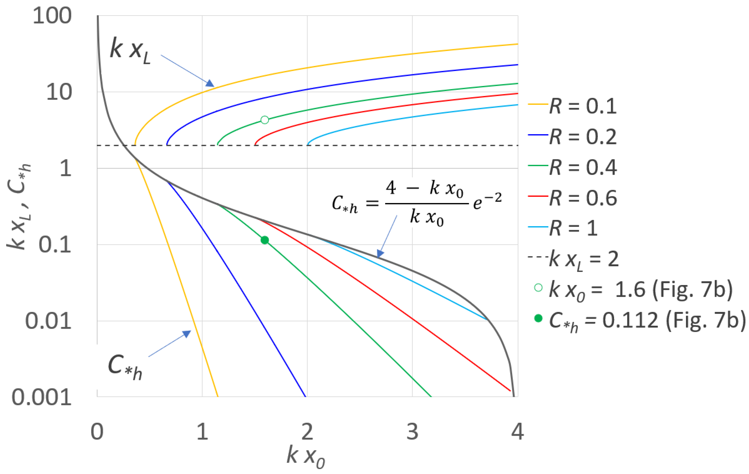
For different R values, Figure 6 plots k x_L (Equation (44)) and C_*h (Equation (36)) as a function of k x₀. The limiting conditions (k x_L)_th = 2 and Equation (38) are also illustrated. As expected, for any selected SS sample (v₀ and k), an increase in the influent SS concentration (k x₀) determines a k x_L increase but also requires decreasing C_*h—i.e., decreasing Q—or increasing the clarifier surface area (for the design purpose) or the return ratio. Figure 3, Figure 4 and Figure 6 strongly evidence its general validity for all the design/verification parameters’ combinations.

2.5. The Domains of the SS Concentration and of the Solid Flux

As observed in Section 2, x_min delimits the biomass concentration domain (x_min ≤ x ≤ x_L), which can even be analyzed in dimensionless terms by varying u_*. The possible domain of the biomass concentration, Δx_*, and the corresponding solid flux domain, ΔG_*, are expressed by the following:

$$\mathrm{\Delta }{x}_{\ast }=k x_L-k x_{min}$$

(45)

$$\mathrm{\Delta }{G}_{\ast }=G_{\ast max}-G_{\ast L}$$

(46)

After simple algebra, calculating k x_min by replacing W₋₁ with W₀ in Equation (21), using Equation (24) to calculate G_*max and G_*L, and substituting into Equation (45) and Equation (46) provides Δx_* and ΔG_* relationships that only depend on W₋₁ and W₀:

$$\mathrm{\Delta }{x}_{\ast }=W_0\left(-\mathrm{e} u_{\ast }\right)-W_{-1}\left(-\mathrm{e} u_{\ast }\right)$$

(47)

$$\mathrm{\Delta }{G}_{\ast }=u_{\ast }\left[W_{-1}^{-1}\left(-\mathrm{e} u_{\ast }\right)-W_0^{-1}\left(-\mathrm{e} u_{\ast }\right)-\mathrm{\Delta }{x}_{\ast }\right]$$

(48)

Figure 7a plots Equations (47) and (48) (secondary axis) versus u_*. As expected, both Δx_* and ΔG_*, in between which the pairs (k x₀, G_*) could lay, decrease at increasing u_*, meaning that for high u_*, WWTP misoperation could be expected, depending on the occurring variable influent SS concentration. Of course, for u_* = u_*th = 0.1353 (Table 1), Δx_* and ΔG_* are equal to zero. In Figure 7a, the black dots correspond to the parameters Δx_* and ΔG_* of the application performed in the next section (Figure 7b).

3. Example of Application

In this section, a numerical application of the described procedure is described. The involved parameters are summarized in

Table 2. Dimensional parameters and their symbols and values, corresponding to the application of Figure 7b.

Dimensional Parameters	Symbol	Value
Settling velocity under zero SS concentration (x = 0)	v0 (m h−1)	8.0
Exponential decay constant	k (m3 kg−1)	0.375
Virtual solids flux under zero SS concentration (x = 0, v = v0)	G0 (kg m−2 h−1)	21.35
Influent SS concentration to the final clarifier	x0 (kg m−3)	4.27
Settling velocity for settling velocity for x = x0	v (x0) (kg m−3)	1.62
Total solid flux for x = x0	G (x0) (kg m−2 h−1)	8.43
Influent discharge to the treatment plant	Q (m3 h−1)	54.0
Return sludge discharge	Qr (m3 h−1)	21.6
SS concentration of the recycle flowrate	xr (kg m−3)	14.94
Recycle velocity	u (m h−1)	0.359
Limiting SS concentration	xL (kg m−3)	11.47
Limiting solids flux	GL (kg m−2 h−1)	5.37
Total solid flow to the final clarifier	(Q + Qr) x0 (kg h−1)	322.8
Clarifier surface area	A (m2)	60.16
Hydraulic loading rate	Ch (m h−1)	0.90

in dimensional terms and in

Table 3. Dimensionless groups and their symbols and values, corresponding to the application of Figure 7b.

Dimensionless Parameters	Symbol	Value
Return ratio	R	0.40
Recycle velocity, u, normalized with respect to v0	u*	0.045
Dimensionless influent SS concentration	k x0	1.600
Dimensionless limiting SS concentration	k xL	4.297
Limiting solids flux normalized with respect to G0	G*L	0.251
Dimensionless SS concentration of the recycle flowrate	k xr	5.600
Hydraulic loading rate normalized with respect to v0	C*h	0.112

in a far smaller number of dimensionless terms.

For verification purposes, let us assume that a WWTP is fed by an influent discharge Q equal to 54 m³ h⁻¹ and operates with a return ratio R = 40%, so that the return sludge discharge Q_r equals 21.6 m³ h⁻¹. The parameters k and v₀ of the Vesilind model are equal to 8 m h⁻¹ and 0.375 m³ kg⁻¹, respectively, and the clarifier surface area A is 60.16 m². By assuming ρ = 1 for an influent SS concentration to the final clarifier of x₀ = 4.27 kg m⁻³ (k x₀ = 1.6), we want to establish whether the WWTP operates properly—i.e., the solids do not escape in the supernatant—and how the WWTP operates under R or x₀ variability.

Equation (14), u_* = R Q/(v₀ A), equals 0.045, which for e u_* = 0.122 (W₋₁ = −3.3, Figure 2) allows calculating k x_L by Equation (21) (Figure 3), resulting to 4.297. Thus, k x_L is properly higher than (k x_L)_th = 2. Knowing u_* makes it possible to calculate G_*L = 0.251 and k x_r = 5.6, which are also indicated in Figure 3. The goodness of the WWTP design can also be observed in Figure 4a, where for k x₀ = 1.6, the pair (R = 0.4, k x_L = 4.297) is illustrated, together with the limiting condition.

The effect of k x₀ and R variation can be observed in Figure 4a and Figure 5a, and in Figure 6, where the considered parameters, k x₀ = 1.6 and R = 0.4, match those of this application, and the corresponding dots are indicated. In Figure 5a, it can be observed that at increasing R, C_*h, which for x = x₀ equals 0.112, increases too, meaning that for the fixed clarifier surface area, A = 60.16 m², a higher influent discharge, Q, to the WWTP should be required. Meanwhile, for a fixed R = 0.4 at increasing k x₀, Figure 5a shows that C_*h decreases, and so should Q.

Finally, for an influent SS concentration to the final clarifier corresponding to the limiting condition (k x₀ = k x_L), the normalized settling velocity, v/v₀, highly decreases (from 0.202 to 0.014), and for the imposed Q, the clarifier surface area should be 161.55 m²—thus 2.68 times greater than for x = x₀ (Table 2).

The dimensionless parameters of this example application (Table 3) make it possible to illustrate the normalized solids fluxes G_*v and G_*u and their sum G_* (Equation (1)) versus the normalized biomass concentration, k x, as graphed in Figure 7b. Figure 7b also shows the normalized solid fluxes corresponding to both k x₀ = 1.6 and k x_L = 4.3, in green and red dots, respectively. The minimum value of the biomass concentration x_min, associated with G_max, and the domains Δx_* and ΔG_* are also displayed in Figure 7b.

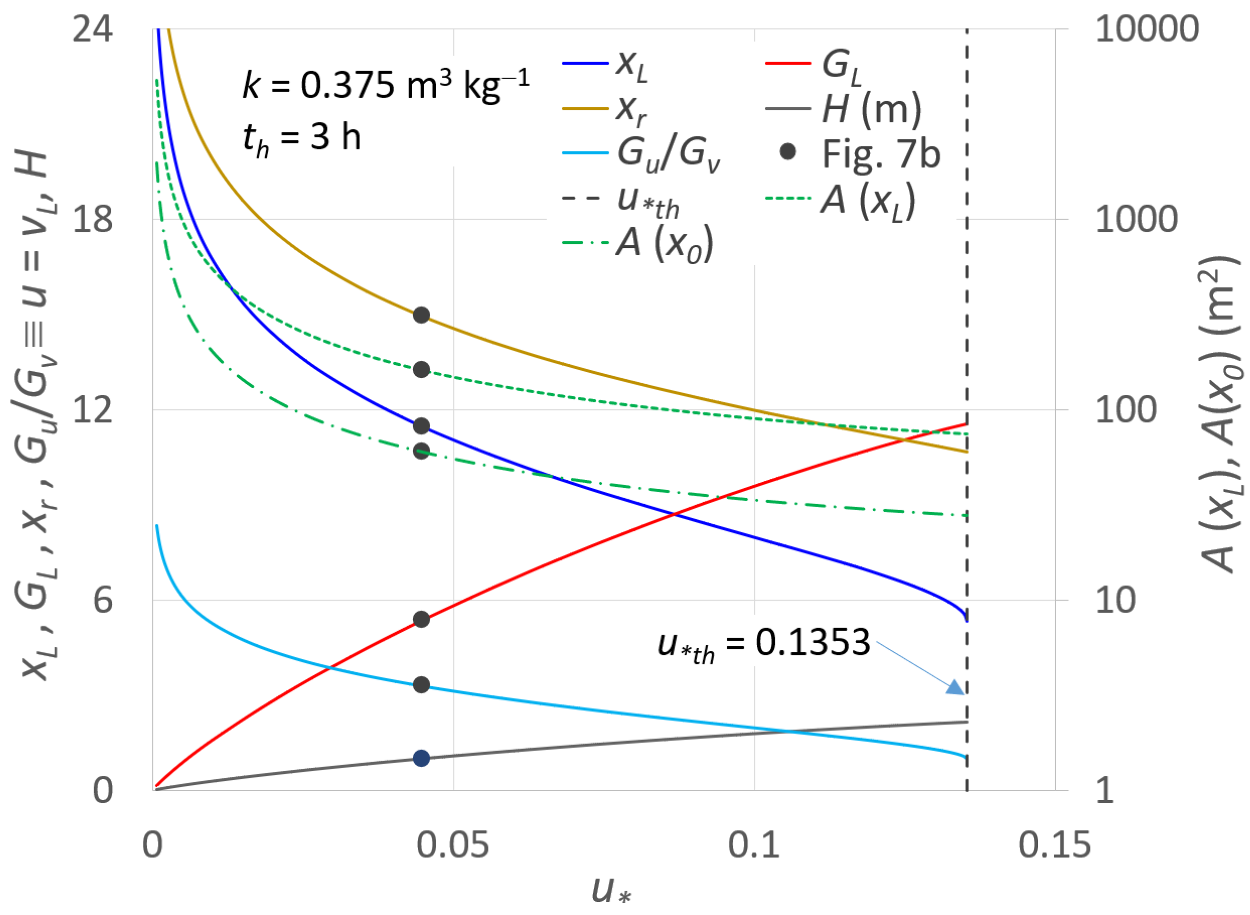
Once the verification problem, or the design problem, is solved in dimensionless terms, for the considered case, the dimensional variables can be easily derived by calculating G₀ = v₀/k (Equation (22)), which is equal to 21.35 kg m⁻² h⁻¹. In dimensional terms, for the imposed influent discharge Q = 54 m³ h⁻¹, Figure 8 shows the expected decreasing trends versus u_* of x_L, x_r, and G_u/G_v in the secondary axis for x = x_L and x = x₀, A(x_L) and A(x₀), respectively, and the increasing trend of G_L.

By assuming a hydraulic detention time of t_h = 3 h (i.e., clarifier volume V = Q t_h = 162 m³), the height of the final clarifier, H, versus u_* is also graphed. For any u_* value, the clarifier surface area corresponding to x₀ = 4.27 kg m⁻³, A(x₀), provides lower values than A(x_L). The parameters corresponding to the application of Figure 7b are indicated by black dots.

Figure 8 makes it possible to elucidate the influence of the recycling flow rate on the design parameters. The ratio G_u/G_v ≥ 1 which matches the ratio u/v_L is interesting to consider since it represents how much higher the involved recycling flow rate, related to the energy required for recycling, is than the gravitational settling velocity. Of course, for u = u_th, the ratio G_u/G_v ≡ u/v_v is equal to the unity. This occurrence is seldom achieved in practice since it is associated with low x_L values and high values of the settling velocity. Moreover, for u > u_th, the energy required for the sludge extraction would be less than that corresponding to the gravitational hindered settling, but high u values make the wastewater treatment not efficient from an energetic point of view. In practice, high u values also need to be checked according to the required cellular residence time, depending on the wastewater characteristics.

From an economic point of view, the most convenient design choice should be performed by also considering the energy and the investment costs. Since at increasing u the former increases and the latter decreases, the design choice corresponding to the maximum economic benefit could be detected. However, the latter issue is beyond the scope of this work.

4. Comparison with Experimental Data and the New Hydrodynamic Factor

Experimental data retrieved from the literature [34] were used to verify the suitability of the detected dimensionless groups, as well as for the evaluation of the reduction hydrodynamic factor. D’Antonio and Carbone [34] verified the SFT by experimental measurements carried out in a treatment pilot plant (0.4 m in diameter and 1.5 m high) in Bagnoli (IT) for influent SS concentrations to the final clarifier equal to x₀ = 1.8, 2.3, 3.0, and 3.8 kg m⁻³, which correspond to k x₀ = 0.864, 1.104, 1.440, and 1.840, respectively, for the k = 0.48 m³ kg⁻¹ Vesilind parameter that we considered.

By using power and exponential laws to describe the sedimentation model, d’Antonio and Carbone [34] identified in the exponential law the best function that interprets the behavior of the sedimentation tank and concluded that the use of theoretical equations derived by SFT produced an undersized value of 30% of the surface area on average and of 15% according to the values of the underflow withdrawal velocity.

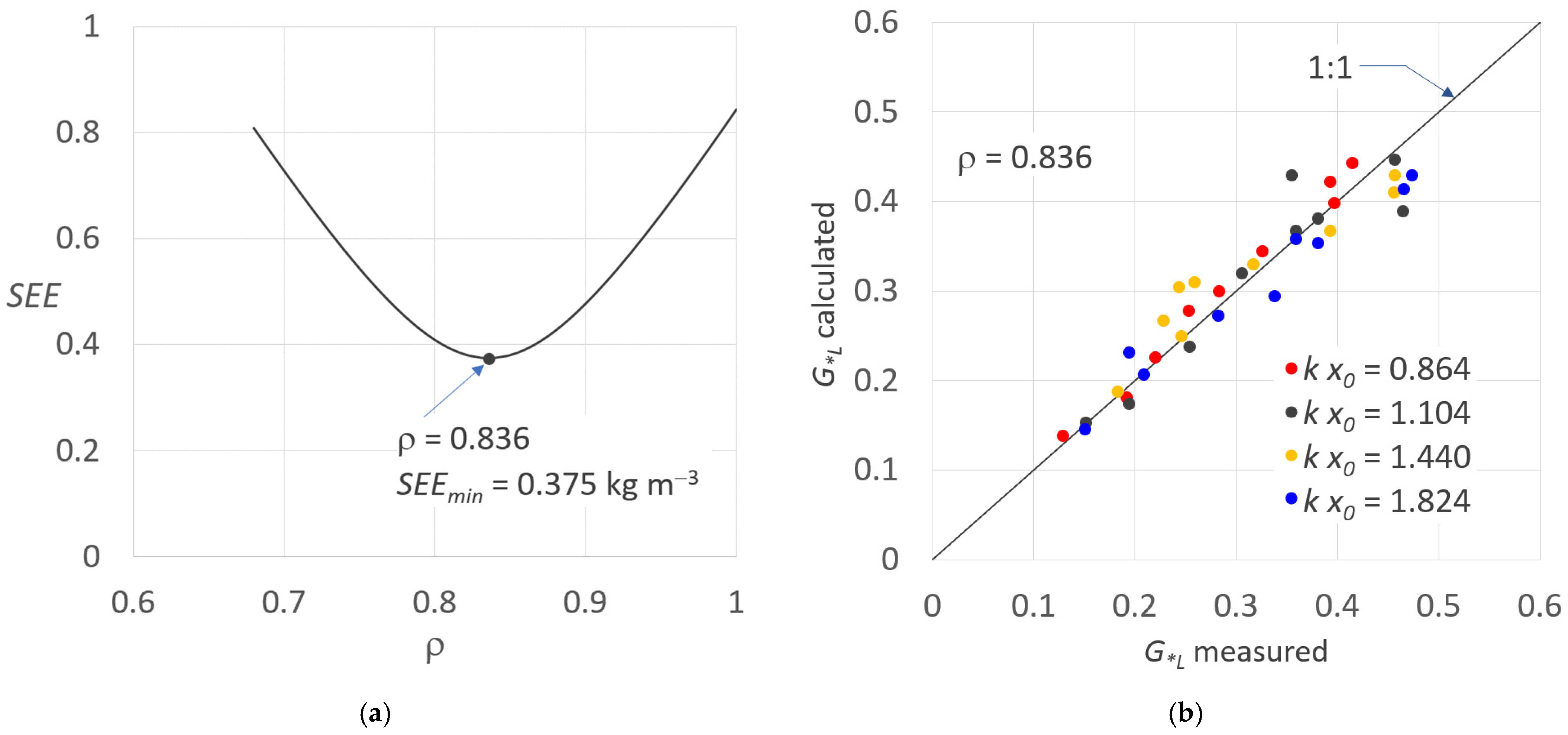
The experimental limiting solid fluxes and the hydraulic loading rates provided by d’Antonio and Carbone [34] were considered in this work. First, by varying the reduction hydrodynamic factor ρ, the standard error on the estimate, SEE, between the experimental limiting normalized solid fluxes, G_*L,m,i, and those calculated by Equation (24) was determined:

$$SEE=\sqrt{{\sum }_{i=1}^N\frac{{\left(G_{\ast L,m,i}-\mathsf{\rho } {\left(k x_{L,i}\right)}^2 e^{-k x_{L,i}}\right)}^2}{N-1}}$$

(49)

where N is the sample size, which is equal to 36 and refers to the runs carried out for u_* < u_*th. The SEE values are plotted in Figure 9a, showing that for ρ = 0.836, the minimum SSE, SSE_min = 0.0856, was obtained (

Table 4. Sum square error, SSE; sample size, N; and standard error of the estimate, SEE, for different values of the reduction hydrodynamic factor.

Correction Factor	ρ Estimation Method	SSE	N	SEE
ρ = 1	no correction in the SFT, Figure 10a	0.2492	35	0.0856
ρ = 0.836	by minimizing SSE (GL), Figure 10b	0.0862	35	0.0448
ρ = 0.809	by minimizing SSE (C*h), Figure 11a	0.0640	35	0.0434
ρR = 0.796	by minimizing SSE (C*h), Figure 11b	0.0688	49	0.0378

).

For ρ = 0.836, the comparison between the observed and calculated G_*L values is plotted in Figure 9b, with k x₀ as a parameter. The obtained ρ values almost agree with the results found by other researchers such as Ekama and Marais [42] and Gohle et al. [43], who suggested ρ = 0.8. Watts et al. [32] also found ρ values in the range of 0.55–0.94, with an average of ρ = 0.73.

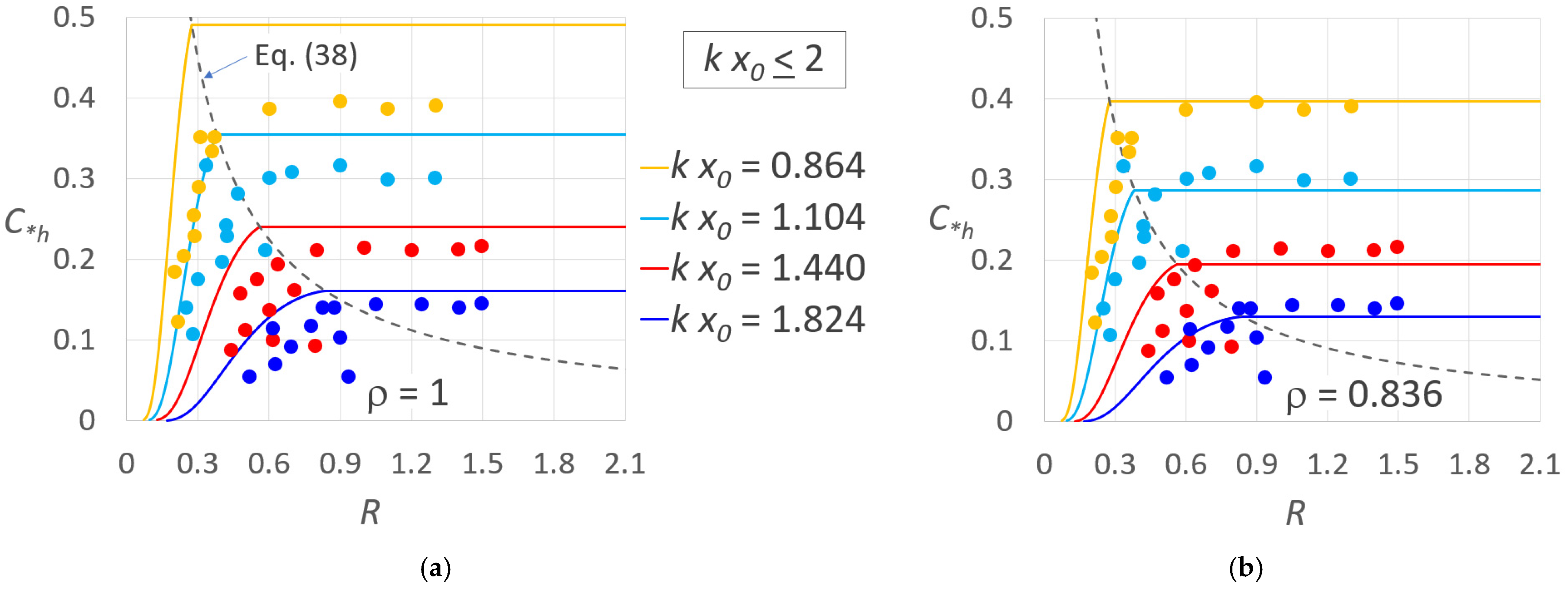
The consistency of the detected ρ values can also be observed by comparing Figure 10a,b, where the normalized hydraulic rate C_*h versus R is graphed (Equation (36)) together with the corresponding experimental values derived by d’Antonio and Carbone (1987) for ρ = 1 (Figure 10a, no correction) and for ρ = 0.836 (Figure 10b), with k x₀ as a parameter.

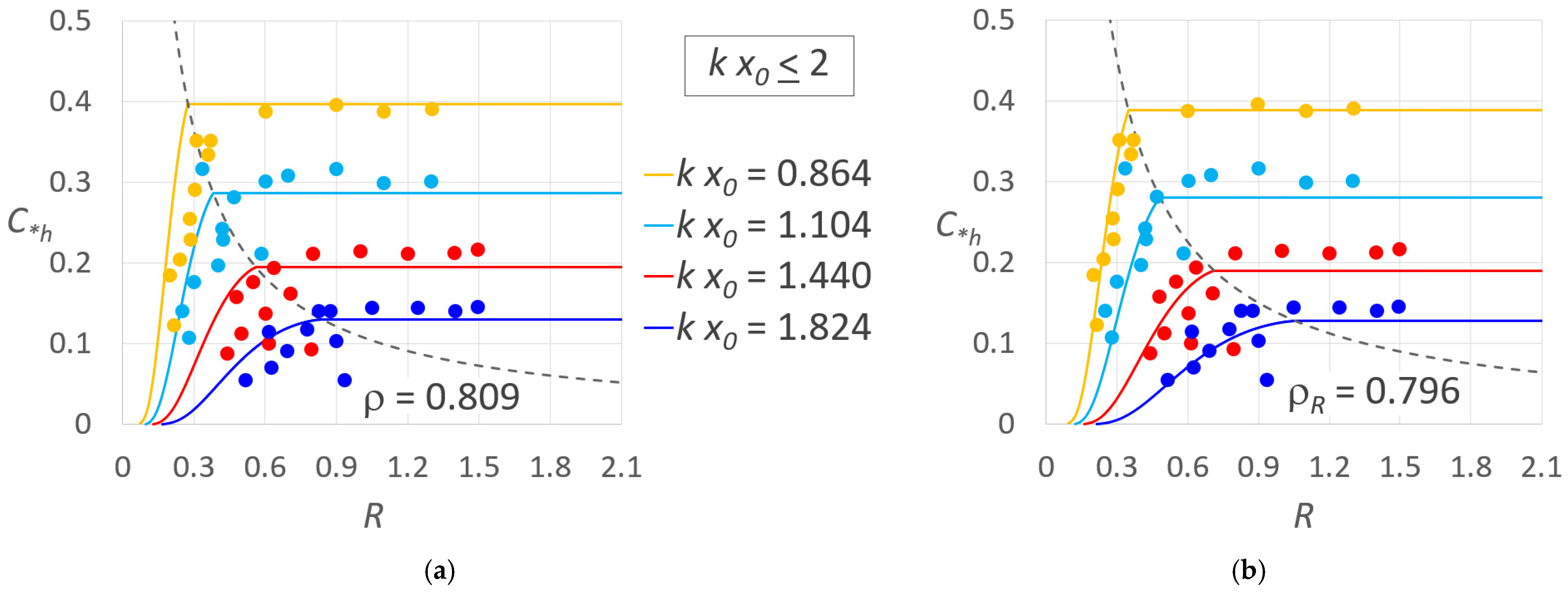
A slight improvement in the results displayed in Figure 10b was obtained by minimizing the SSE for the whole dataset provided by d’Antonio and Carbone (1987), including the 36 C_h measurements carried out for u_* < u_*tk and the 18 measurements carried out for u_* > u_*th (Figure 11a), yielding ρ = 0.809.

Based on the rationale that the hydrodynamic factor applied to G_*L only partially corrects the simplified SFT, another attempt was made to improve the accuracy of the predictions derived by the SFT because according to Equation (24), k x_L, which affects the other design variables, certainly also requires correction.

Differently from the above-mentioned researchers [32,42,43], who applied the correction factor ρ to the limiting solid flux, it is opinion of these authors that the correction could be applied to the return ratio R. This is because the dependence of G_*L on k x_L is not linear; applying a correction to R by introducing a new reduction hydrodynamic factor, ρ_R, into Equation (29) would overcome this issue:

$$R={\mathsf{\rho }}_R\frac{k x_0\left(k x_L-1\right)}{{\left( k x_L\right)}^2-k x_0\left(k x_L-1\right)}$$

(50)

The results obtained by applying Equation (50) with ρ_R = 0.796 and Equation (36) with ρ = 1 strongly improved the fitting of the experimental measurements to the new dimensionless SFT (especially for k x₀ = 0.864), as can be observed in Figure 11b. The corresponding SEE values seem to validate the new ρ_R hydrodynamic factor to be applied to Equation (50) since for this scenario, the lowest SEE = 0.0378 was obtained (Table 4).

5. Conclusions

Activated sludge processes are the most widely used biological processes in wastewater treatment plants (WWTPs) and are based on the well-known solid flux theory. In this paper, by adopting the widespread Vesilind sedimentation model, the solid flux theory has been reformulated according to a “virtual” solid flux corresponding to the Vesilind parameters’ ratio and dimensionless groups that consolidate the parameters that are involved in a far smaller number of parameters.

The Lambert W function, which helps detect the limiting solid flux and the domains of the normalized biomass concentration and the solid flux, was applied and suggested that the key parameter is the limiting dimensionless SS concentration, which was found to be related to the other design parameters, thus greatly simplifying the design procedure of the final clarifier.

It was shown that the plots obtained by the derived dimensionless relationships have general validity and describe all the possible design parameter combinations. Numerical applications and validations of the dimensionless relationships using data retrieved from the literature were performed.

Finally, it is suggested that by introducing in the solid flux theory a reduction hydrodynamic factor to be applied to a new return flow formula rather than to the limiting solid flux as in the past, a significant improvement in the comparison between results by theory and those by experiments can be obtained, since the standard error on the normalized hydraulic loading rate estimate moved from 0.0856 to 0.0378.

References

- Gray, N.F. Activated Sludge, Theory and Practice; Oxford University: Oxford, UK, 1990. [Google Scholar]
- Yang, Y.; Wang, L.; Xiang, F.; Zhao, L.; Qiao, Z. Activated Sludge Microbial Community and Treatment Performance of Wastewater Treatment Plants in Industrial and Municipal Zones. Int. J. Environ. Res. Public Health 2020, 17, 436. [Google Scholar] [CrossRef] [PubMed] [Green Version]
- Puig, S.; van Loosdrecht, M.C.M.; Colprim, J.; Meijer, S.C.F. Data evaluation of full-scale wastewater treatment plants by mass balance. Water Res. 2008, 42, 4645–4655. [Google Scholar] [CrossRef] [PubMed]
- EEA. European Environment Agency. Urban Waste Water Treatment for 21st Century Challenges. 2019. Available online: https://www.eea.europa.eu/highlights/new-challenges-facing-europe2019s-wastewater (accessed on 12 August 2022).
- Abu-Madi, M.O.R. Incentive Systems for Wastewater Treatment and Reuse in Irrigated Agriculture in the MENA Region: Evidence from Jordan and Tunisia; CRC Press: Boca Raton, FL, USA; Taylor and Francis Group: London, UK, 2004. [Google Scholar]
- Keinath, T.M. Operational dynamics and control of secondary clarifiers. J. Water Pollut. Control Fed. 1985, 57, 770–776. [Google Scholar]
- Chancelier, J.P.; de Lara, M.C.; Joannis, C.; Pacard, F. New insight in dynamic modelling of a secondary settler—I. Flux theory and steady-states analysis. Water Res. 1997, 31, 1847–1856. [Google Scholar] [CrossRef]
- Ekama, G.A.; Barnard, J.L.; Günthert, F.W.; Krebs, P.; McCorquodale, J.A.; Parker, D.S.; Wahlberg, E.J. Secondary Settling Tanks: Theory, Modelling, Design and Operation; IAWQ Scientific and Technical Report No. 6; IWA Publishing: London, UK, 1997. [Google Scholar]
- Ozinsky, A.E.; Ekama, G.A.; Reddy, B.D. Mathematical Simulation of Dynamic Behaviour of Secondary Settling Tanks; Technical Report W85; Department of Civil Engineering, University of Cape Town: Cape Town, South Africa, 1994. [Google Scholar]
- Jasim, N.A. The design for wastewater treatment plant (WWTP) with GPS X modelling. Cogent Eng. 2020, 7, 1723782. [Google Scholar] [CrossRef]
- Islam, M.A.; Amin, M.S.A.; Hoinkis, J. Optimal design of an activated sludge plant: Theoretical analysis. Appl. Water Sci. 2013, 3, 375–386. [Google Scholar] [CrossRef] [Green Version]
- Vitasovic, Z. Continuous Settler Operation: A Dynamic Model Dynamic Modeling and Expert Systems in Wastewater Engineering; Patry, G.G., Chapman, D., Eds.; Lewis Publishers: Boca Raton, FL, USA, 1989. [Google Scholar]
- Koehne, M.; Hoen, K.; Schuhen, M. Modelling and simulation of final clarifiers in wastewater treatment plants. Math. Comput. Simul. 1995, 39, 609–616. [Google Scholar] [CrossRef]
- Kim, H.S.; Shin, M.S.; Janga, D.S.; Jung, S.H.; Jin, J.H. Study of flow characteristics in a secondary clarifier by numerical simulation and radioisotope tracer technique. Appl. Radiat. Isot. 2005, 63, 519–526. [Google Scholar] [CrossRef]
- Kynch, G.J. A theory of sedimentation. Trans. Faraday Soc. 1952, 48, 166–176. [Google Scholar] [CrossRef]
- Yuen, W.A. Empirical Equations for the Limiting Solids Flux of Final Clarifiers. Water Environ. Res. 2002, 74, 2. [Google Scholar] [CrossRef]
- Daigger, G.T. Development of Refined Clarifier Operating Diagrams Using an Updated Settling Characteristics Database. Water Environ. Res. 1995, 67, 95. [Google Scholar] [CrossRef]
- Daigger, G.T.; Roper, R.E. The relationship between SVI and activated sludge settling characteristics. J. Water Pollut. Control Fed. 1985, 57, 859–866. [Google Scholar]
- Hermanowicz, S.W. Secondary Clarification of Activated Sludge: Development of Operating Diagrams. Water Environ. Res. 1998, 70, 10. [Google Scholar] [CrossRef]
- Keinath, T.M. Diagram for Designing and Operating Secondary Clarifiers According to the Thickening Criterion. J. Water Pollut. Control Fed. 1990, 62, 254. [Google Scholar]
- Koopman, B.; Cadee, K. Prediction of Thickening Capacity Using Diluted Sludge Volume Index. Water Res. 1983, 17, 1427. [Google Scholar] [CrossRef]
- Diehl, S. The solids-flux theory—Confirmation and extension by using partial differential equations. Water Res. 2008, 42, 4976–4988. [Google Scholar] [CrossRef]
- Wang, X.; Zhou, S.; Li, T.; Zhang, Z.; Sun, Y.; Cao, Y. Three-dimensional simulation of the water flow field and the suspended-solids concentration in a circular sedimentation tank. Can. J. Civ. Eng. 2011, 38, 825–836. [Google Scholar] [CrossRef]
- Wett, B. A straight interpretation of the solids flux theory for a three-layer sedimentation model. Water Res. 2002, 36, 2949–2958. [Google Scholar] [CrossRef]
- Baiamonte, G. Simplified model to predict runoff generation time for well-drained and vegetated soils. J. Irrig. Drain. Eng. ASCE 2016, 142, 04016047. [Google Scholar] [CrossRef]
- Baiamonte, G. Simple Relationships for the Optimal Design of Paired Drip Laterals on Uniform Slopes. J. Irrig. Drain. Eng. 2016, 142, 04015054. [Google Scholar] [CrossRef]
- Lessard, P.; Beck, M.B. Dynamic modeling of the activated sludge process: A case study. Water Res. 1993, 27, 963–978. [Google Scholar] [CrossRef]
- Zhang, Y.; Yin, X.; He, Z.; Zhang, X.; Wen, Y.; Wang, H. Modeling the Activated Sludge—Thickening Process in Secondary Settlers. Int. J. Environ. Res. Public Health 2015, 12, 15449–15458. [Google Scholar] [CrossRef] [PubMed] [Green Version]
- Xu, G.; Yin, F.; Xu, Y.; Yu, H.Q. A force-based mechanistic model for describing activated sludge settling process. Water Res. 2017, 127, 118–126. [Google Scholar] [CrossRef] [PubMed]
- Vesilind, P.A. Design of Prototype Thickeners from Batch Settling Tests. Water Sew. Works 1968, 115, 302. [Google Scholar]
- Cho, S.H.; Colin, F.; Sardin, M.; Prost, C. Settling velocity of activated sludge. Water Res. 1993, 27, 1237–1242. [Google Scholar] [CrossRef]
- Watts, R.W.; Svoronos, S.A.; Koopman, B. One-Dimensional Clarifier Model with Sludge Blanket Heights. J. Environ. Eng. 1996, 122, 1094. [Google Scholar] [CrossRef]
- Vanderhasselt, A.; Vanrolleghem, P.A. Estimation of sludge sedimentation parameters from single batch settling curves. Water Res. 2000, 34, 395–406. [Google Scholar] [CrossRef]
- D’Antonio, G.; Carbone, P. Verifica sperimentale della teoria del flusso solido. Ingegneria Sanitaria 1987, 6, 325–336. (In Italian). Available online: http://www.diia.unina.it/pdf/pubb0546.pdf (accessed on 12 August 2022).
- Von Sperling, M.; Fróes, C.M.V. Determination of the Required Surface Area for Activated Sludge Final Clarifiers Based on a Unified Database. Water Res. 1999, 33, 1887. [Google Scholar] [CrossRef]
- Schuler, A.J.; Jang, H. Density effects on activated sludge zone settling velocities. Water Res. 2007, 41, 1814–1822. [Google Scholar] [CrossRef]
- Corless, R.M.; Gonnet, G.H.; Hare, D.E.G.; Jeffrey, D.J.; Knuth, D.E. On the Lambert W function. Adv. Comput. Math. 1996, 5, 329–359. [Google Scholar] [CrossRef]
- Serrano, S.E. Explicit Solution to Green and Ampt Infiltration Equation. J. Hydrol. Eng. 2001, 6, 336–340. [Google Scholar] [CrossRef]
- Baiamonte, G. Complex Rating Curves for Sharp Crested Orifices for Rectangular or Triangular Weirs under Unsteady Flow Conditions. J. Hydrol. Eng. 2021, 26, 04021005. [Google Scholar] [CrossRef]
- Sanin, F.D.; Clarkson, W.W.; Vesilind, P.A. Sludge Engineering: The Treatment and Disposal of Wastewater Sludges; Destech Pubns: Lancaster, PA, USA, 2011; p. 393. [Google Scholar]
- Mancell-Egala, W.A.S.K.; Kinnear, D.; Jones, K.L.; De Clippeleir, H.; Takács, I.; Murthy, S.N. Limit of stokesian settling concentration characterizes sludge settling velocity. Water Res. 2016, 90, 100–110. [Google Scholar] [CrossRef]
- Ekama, G.A.; Marais, G.V.R. Sludge Settleability. Secondary Settling Tank Design Procedures. J. Water Pollut. Control Fed. 1986, 85, 101. [Google Scholar]
- Gohle, F.; Finnson, A.; Hultman, B. Dynamic Simulation of Sludge Blanket Movements in a Full-Scale Rectangular Sedimentation Basin. Water Sci. Technol. 1996, 33, 89. [Google Scholar] [CrossRef]
Figure 1.
Solids flux contributions due to gravity, Gv, and the activated sludge extraction, Gu, and their sum G (Equation (1)) versus the biomass concentration, x, for (a) u = 0.5 m h−1, (b) u = 1 m h−1, (c) u = 1.5 m h−1, and (d) u = uth = 2.32 m h−1. The limiting SS concentration, xL; the corresponding solid flux, GL; and the SS concentration of the recycle flow rate, xr, are also indicated.
Figure 2.
The two branches of the Lambert W function, W0 and W−1. In the branch W−1, the Lambert W function values corresponding to the application performed later are indicated. The domain of the real xL solutions − e u*th ≤ − e u* ≤ 0 and the dots corresponding to the applications are also reported.
Figure 3.
Relationship between the dimensionless parameters k xL (Equation (21)), G*L (Equation (24)), and k xr (Equation (26)) versus the normalized velocity recycle flow rate u* (a) in a log-log scale and (b) in a linear scale. Dots correspond to the applications performed later. For u* = u*th = 0.1353, the threshold values (k xL)th, (G*L)th, and (k xr)th (Table 1) are also indicated.
Figure 4.
Dimensionless parameters k xL (Equation (29)) versus the return ratio, R, (a) for k x0 ≤ 2 and (b) for k x0 ≥ 2. The limiting k xL conditions (Equations (31) and (32)) are also indicated. In (a), the dot corresponds to the applications performed later.