Sub-pixel Area Calculation Methods for Estimating Irrigated Areas

Abstract
:1. Introduction
2. Methods
- Google earth estimate (IAF-GEE);
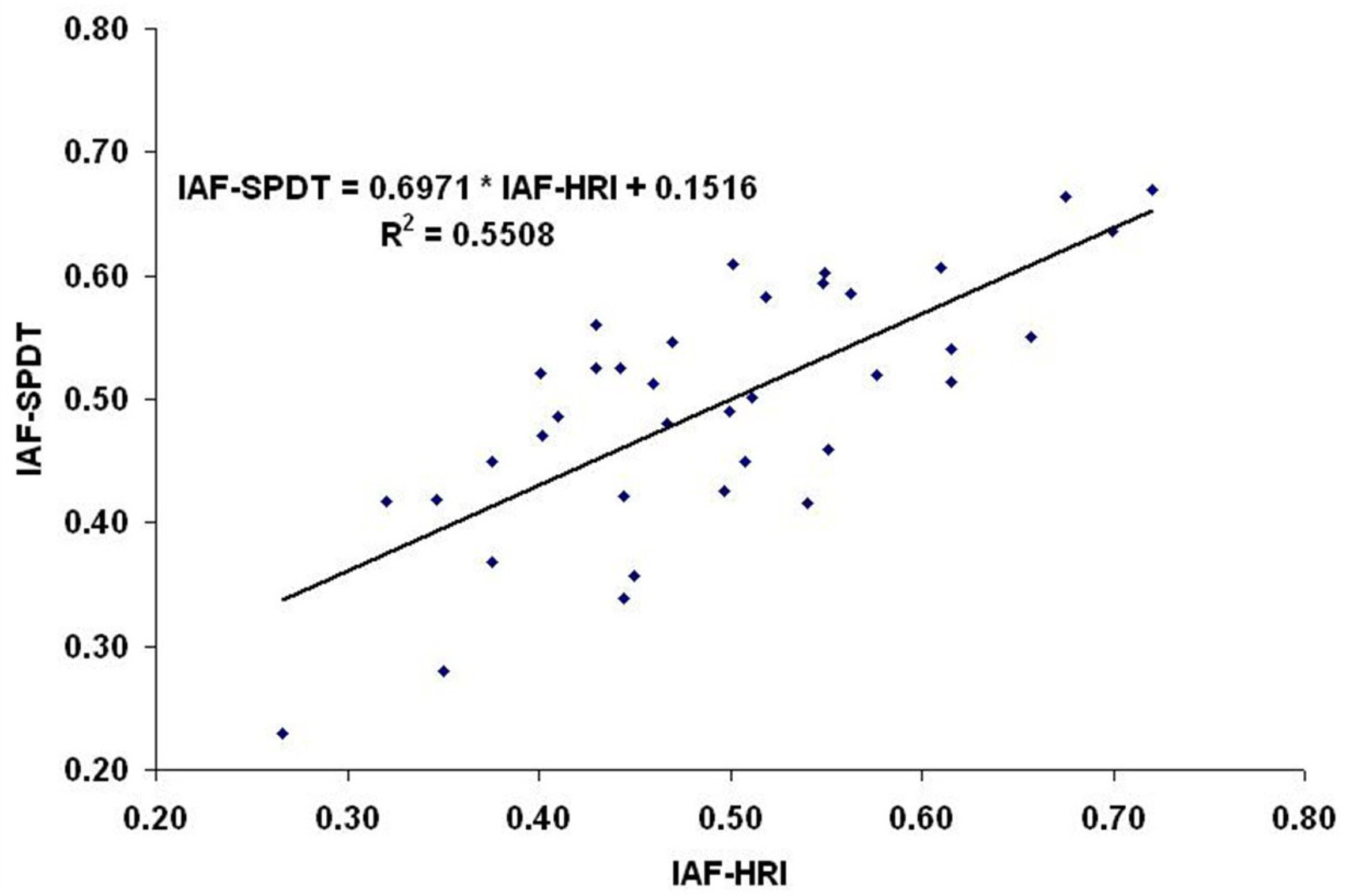
- High resolution imagery (IAF-HRI); and
- Sub-pixel de-composition technique (IAF-SPDT).
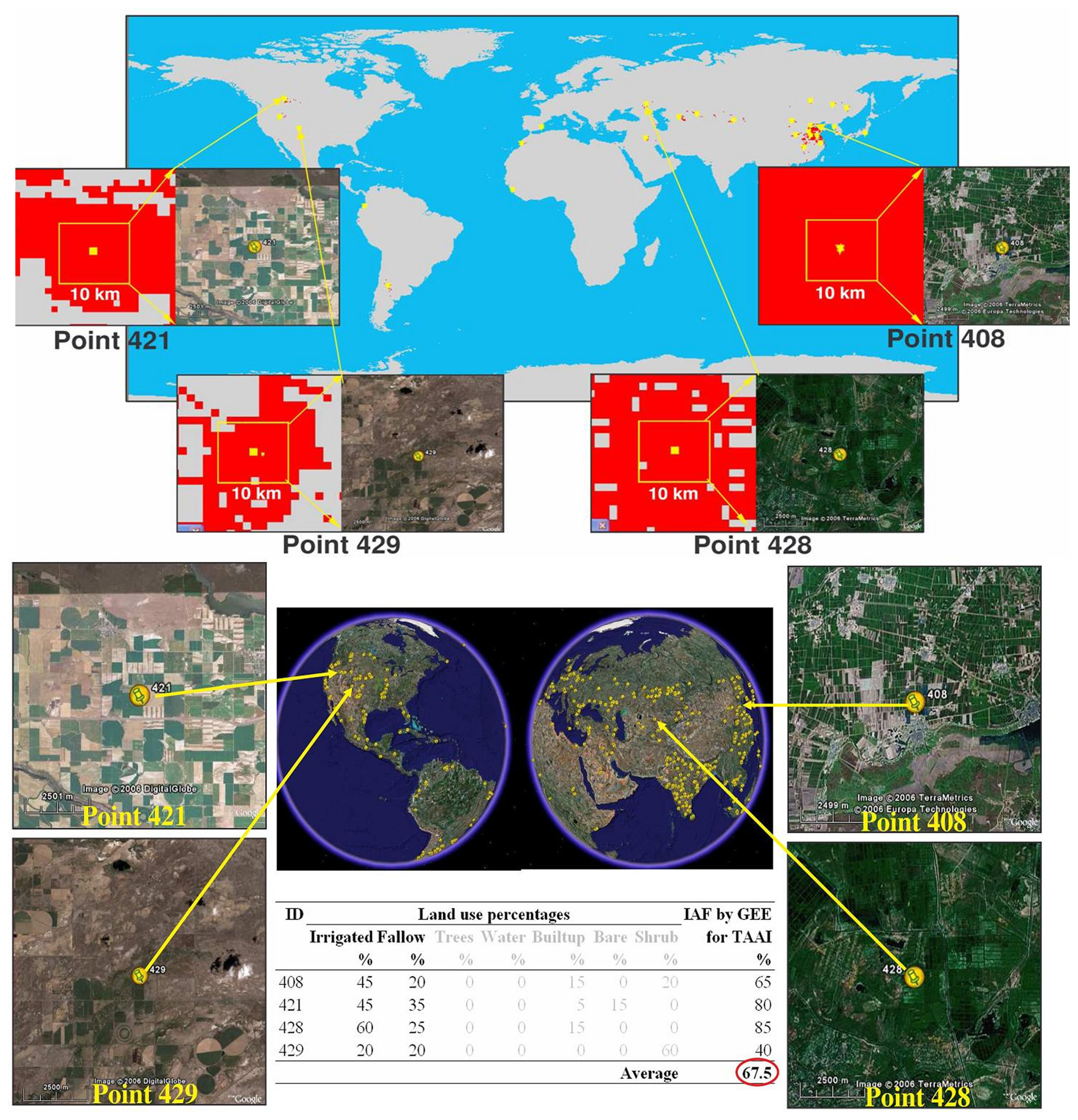
2.1 IAF-GEE
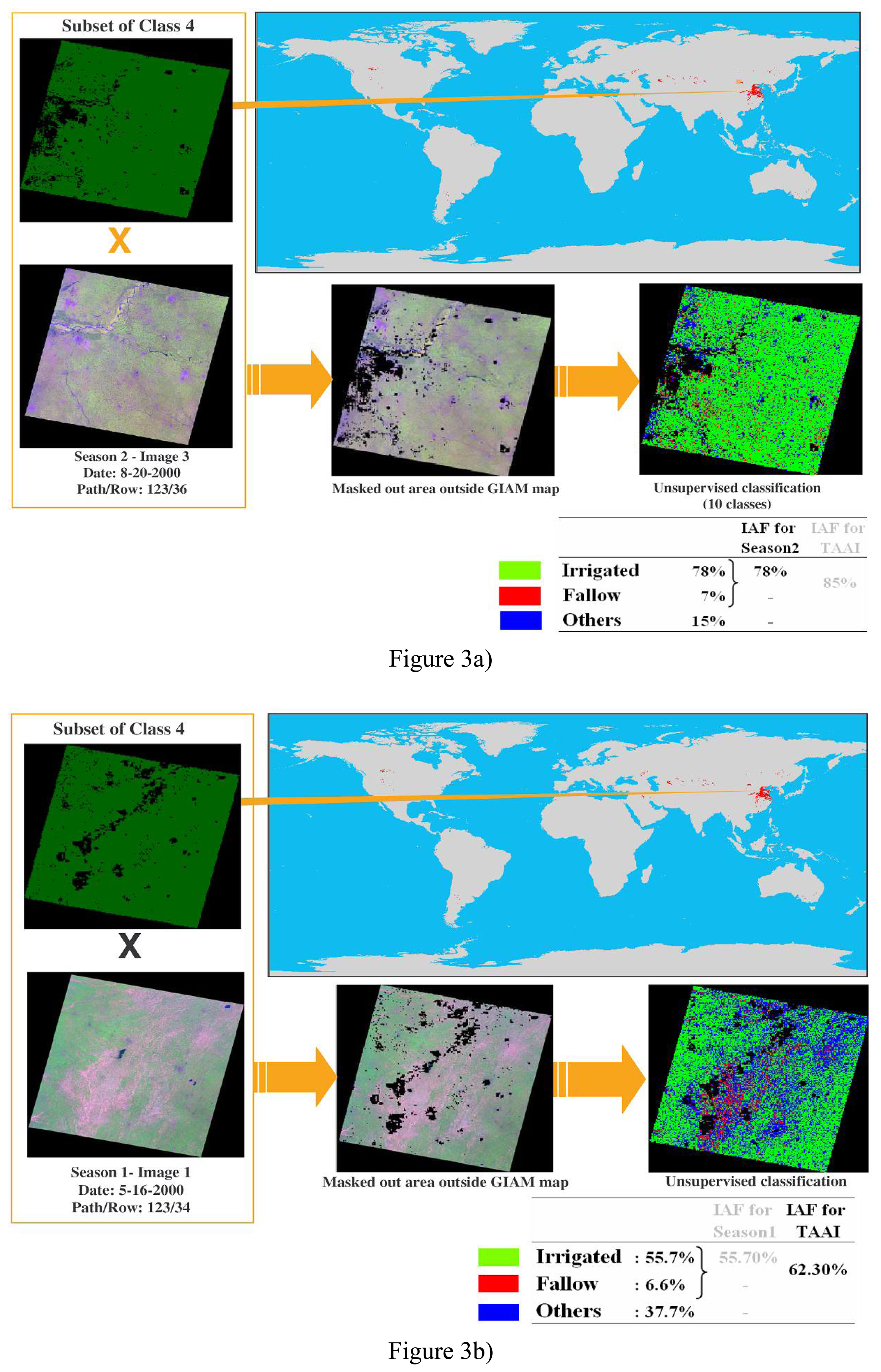
2.2 IAF-HRI
- Randomly selecting 3-6 locations in a GIAM28 class (e.g., illustrated for 1 location in Figure 3a);
- Overlaying Landsat ETM+ 6 band-non-thermal band imagery on GIAM class area and masking out ETM+ imagery area that was outside the GIAM class area (Figure 3a);
- Determine IAF-HRI for the image;
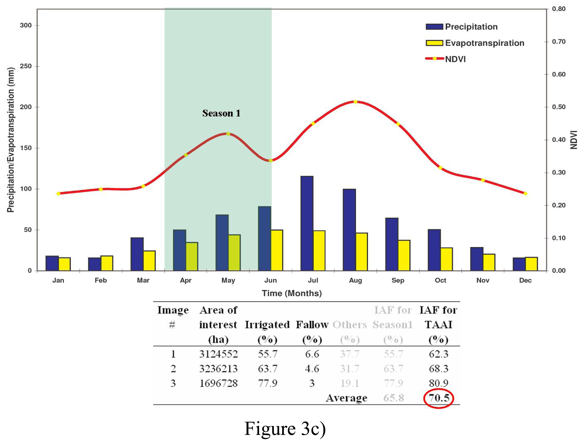
- Repeat the above steps by taking additional Landsat ETM+ images from different portions of the image as well as from different seasons;
- Establish IAF-HRI for each season, by averaging from several images. The resultant fractional irrigated areas shown in Table 1.
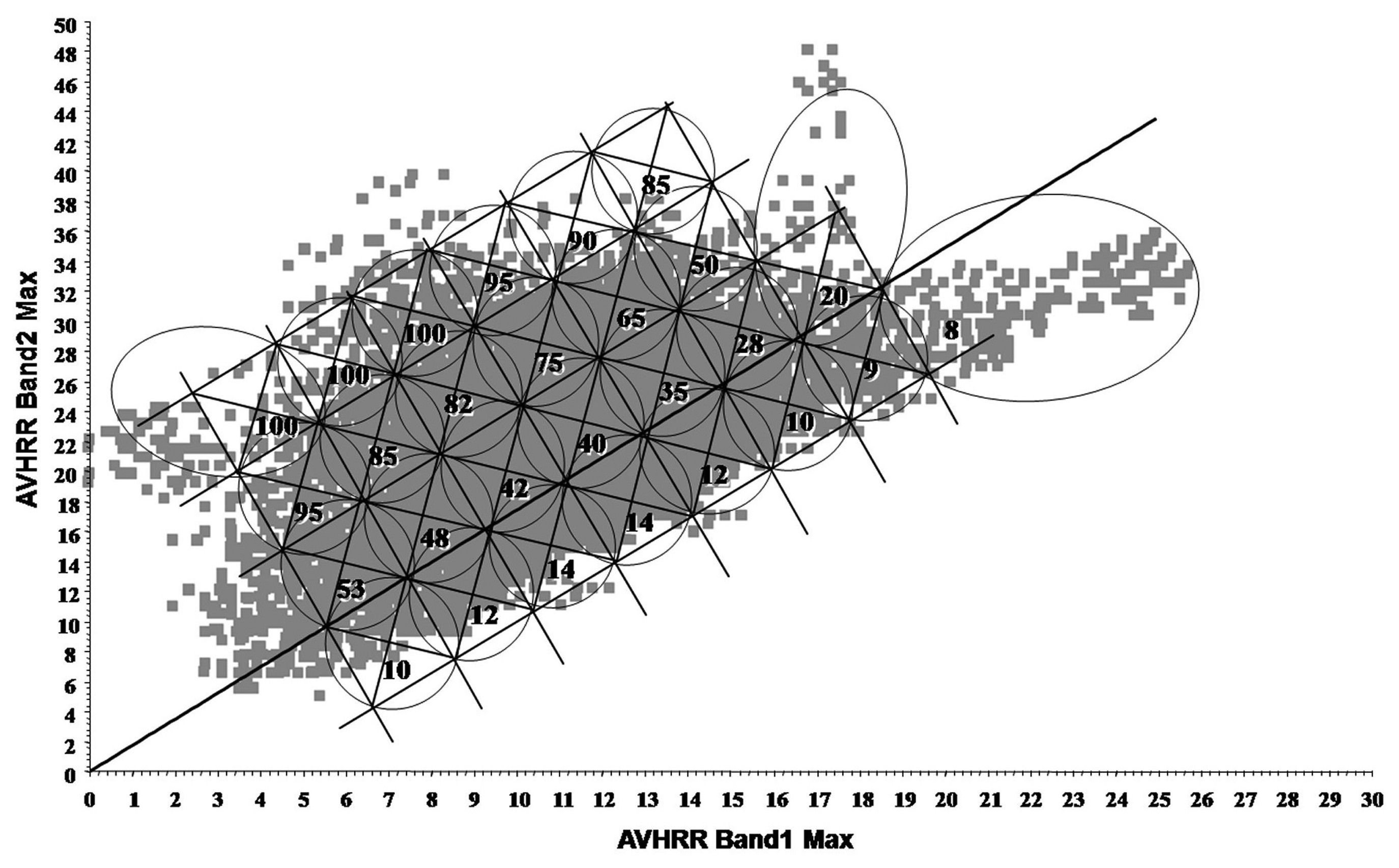
2.3 IAF-SPDT
- groundtruth data and digital photos,
- high-resolution images,
3. SPIAs
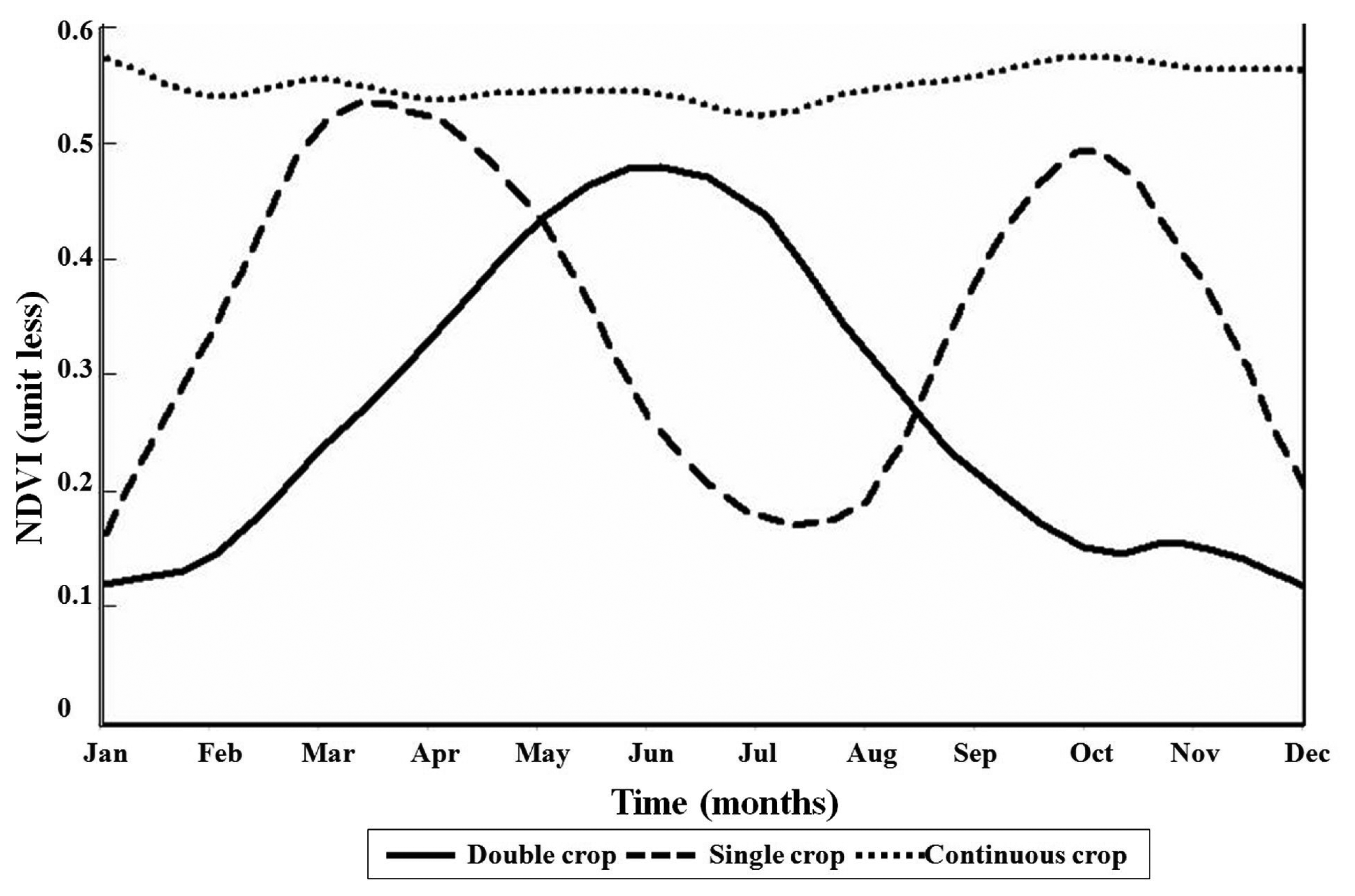
3.1. Total area available for irrigation (TAAI)
3.2 Annualized irrigated area (AIA)
4. Results and Discussion
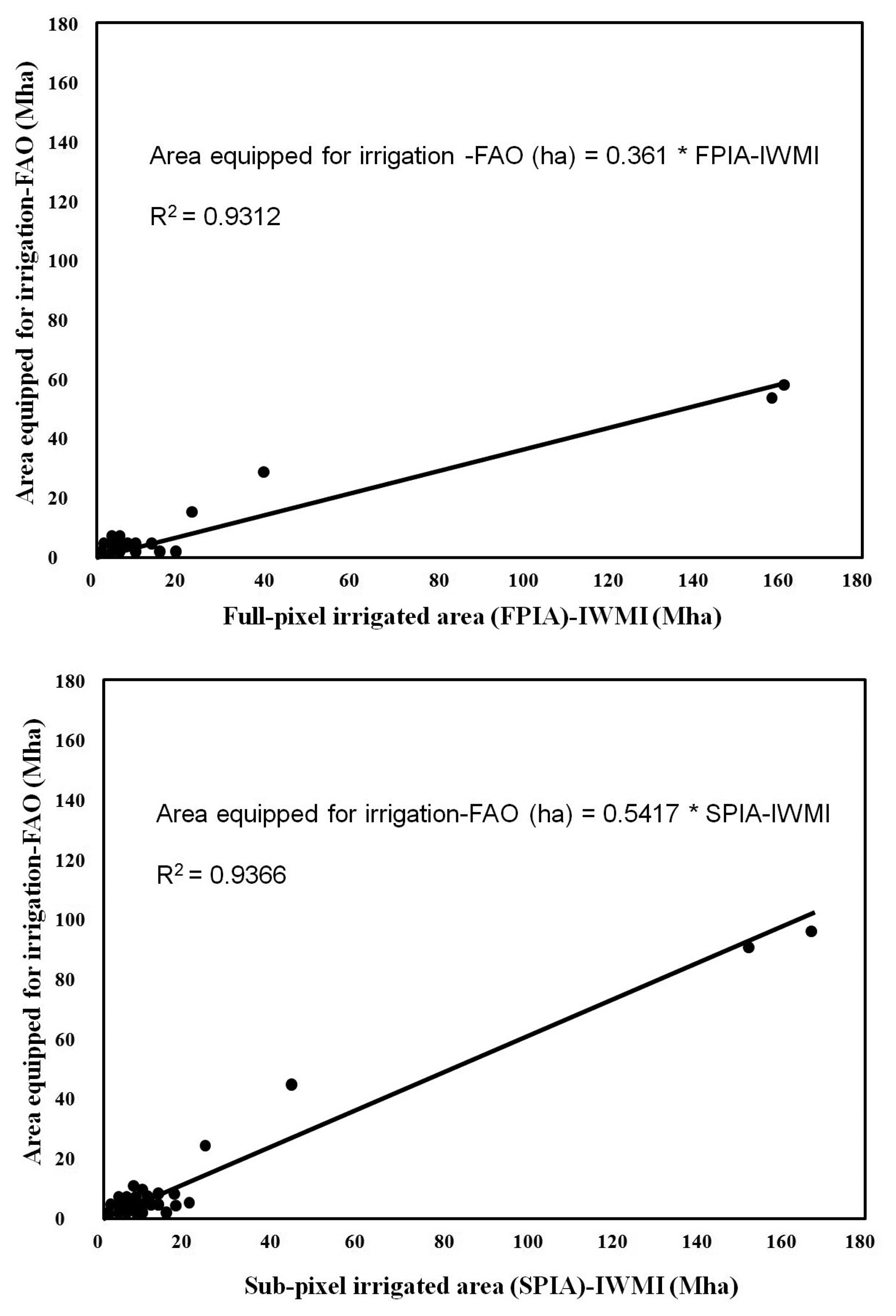
4.1 FPIAs and SPIAs at AVHRR 10-km resolution versus National statistics (FAO Aquastat)
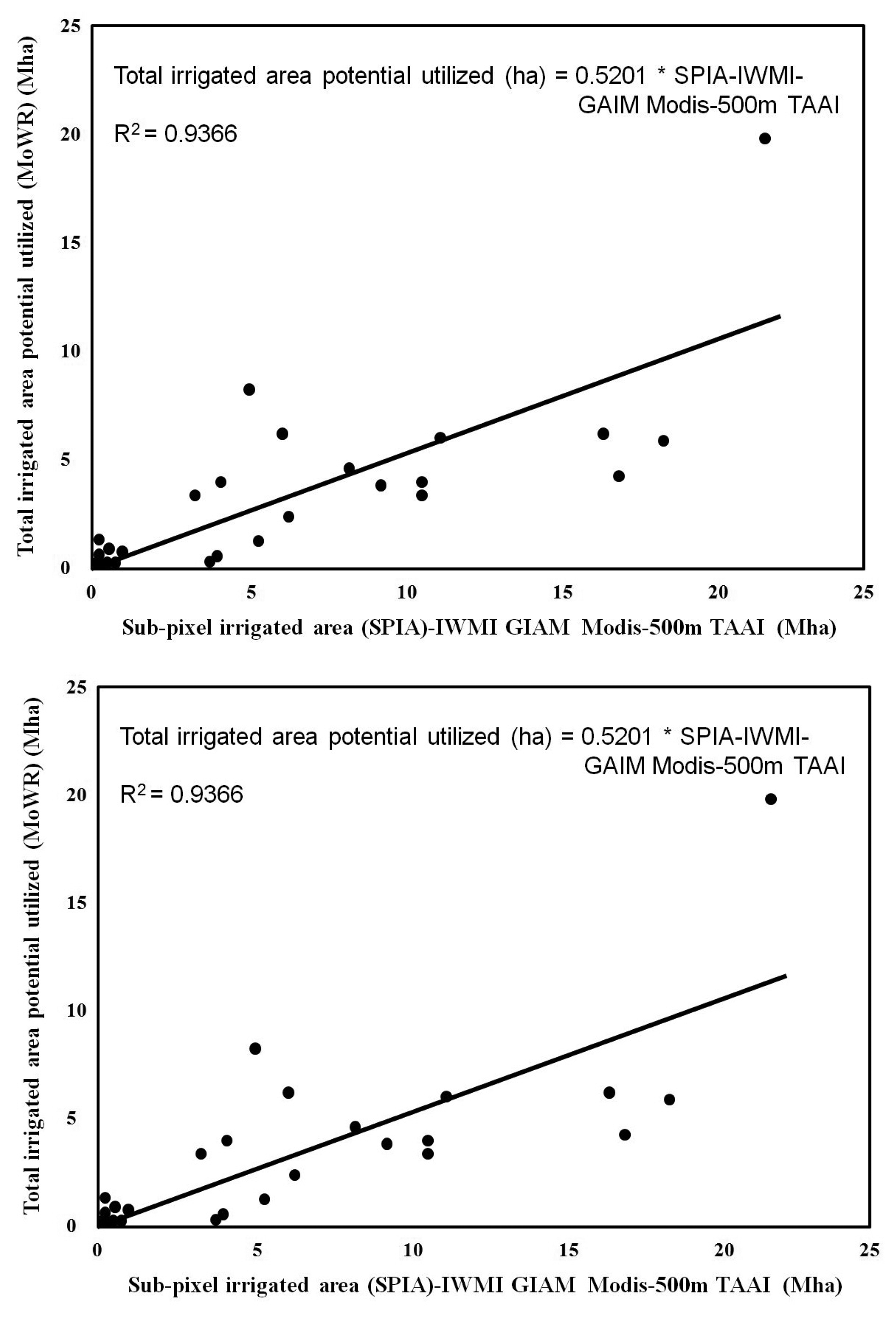
4.2 FPAs and SPAs at MODIS 500-m resolution versus National statistics (FAO Aquastat)
4.3 Uncertainties and errors in SPA estimates
5. Conclusions
6. References and Notes
- Xiao, X.; Liu, J.; Zhuang, D.; Frolking, S.; Boles, S.; Xu, B.; Liu, M.; Salas, W.; Moore, B.; Li, C. Uncertainties in estimates of cropland area in China: a comparison between an AVHRR-derived dataset and a Landsat TM-derived dataset. Global and Planetary Change 2003, 37, 297–306. [Google Scholar]
- Loveland, T.R.; Reed, B.C.; Brown, J.F.; Ohlen, D.O.; Zhu, J.; Yang, L.; Merchant, J.W. Development of a Global Land Cover Characteristics Database and IGBP DISCover from 1-km AVHRR Data. International Journal of Remote Sensing 2000, 21(6-7), 1303–1330. [Google Scholar]
- Gallego, F.J. Remote sensing and land cover area estimation. International Journal of Remote Sensing 2004, 25(15), 3019–3047. [Google Scholar]
- Foody, G.M.; Lucas, R.M.; Curran, P.J.; Honzak, M. Mapping tropical forest fractional cover from coarse spatial resolution remote sensing imagery. Plant Ecology 1997, 131(2), 143–154. [Google Scholar]
- Atkinson, P.M.; Cutler, M.E.J.; Lewis, H. Mapping sub-pixel proportional land cover with AVHRR imagery. International Journal of Remote Sensing 1997, 8(4), 917–935. [Google Scholar]
- Gallego, F.J.; Delince, J.; Rueda, C. Crop area estimates through remote sensing: stability of the regression correction. International Journal of Remote Sensing 1993, 14, 3433–3445. [Google Scholar]
- Gonzalez-Alonso, F.; Cuevas, J.M.; Arbiol, R.; Baulies, X. Remote sensing and agricultural statistics: crop area estimation in north-eastern Spain through diachronic Landsat TM and ground sample data. International Journal of Remote Sensing 1997, 18(2), 467–470. [Google Scholar]
- Thenkabail, P.S.; Biradar, C.M.; Turral, H.; Noojipady, P.; Li, Y.J.; Vithanage, J.; Dheeravath, V.; Velpuri, M.; Schull, M.; Cai, X.L.; Dutta, R. An Irrigated Area Map of the World (1999) derived from Remote Sensing; Research Report No. 105; International Water Management Institute: Battaramulla, Sri Lanka, 2006; p. 74. [Google Scholar]
- Biggs, T.; Thenkabail, P.S.; Krishna, M.; Gangadhara, R.P.; Turral, H. Vegetation phenology and irrigated area mapping using combined MODIS time-series, ground surveys, and agricultural census data in Krishna River Basin, India. International Journal of Remote Sensing 2006, 27(19), 4245–4266. [Google Scholar]
- Fang, H.; Wu, B.; Liu, H.; Huang, X. Using NOAA AVHRR and Landsat TM to estimate rice area year by year. International Journal of Remote Sensing 1998, 19(3), 521–525. [Google Scholar]
- Xiao, X.; Boles, S.; Frolking, S.; Salas, W.; Moore, B.; Li, C.; He, L.; Zhao, R. Landscape-scale characterization of cropland in China using VEGETATION sensor data and Landsat TM imagery. International Journal of Remote Sensing 2002, 23, 3579–3594. [Google Scholar]
- DeFries, R.; Hansen, M.; Steininger, M.; Dubayah, R.; Sohlberg, R.; Townshend, J. Subpixel forest cover in Central Africa from Multisensor, multitemporal data. Remote Sensing of Environment 1997, 60, 226–246. [Google Scholar]
- Quarmby, N.A. Towards continental scale crop area estimation. International Journal of Remote Sensing 1992, 13(5), 981–989. [Google Scholar]
- Ozdogan, M.; Woodcock, C.E. Resolution dependent errors in remote sensing of cultivated areas. Remote Sensing of Environement 2006, 103(2), 203–217. [Google Scholar]
- Thenkabail, P.S.; Schull, M.; Turral, H. Ganges and Indus river basin Land Use/Land Cover (LULC) and irrigated area mapping using continuous streams of MODIS data. Remote Sensing of Environment 2005, 95(3), 317–341. [Google Scholar]
- Thenkabail, P.S.; Gangadhara, R.P.; Biggs, T.; Krishna, M.; Turral, H. Spectral Matching Techniques to Determine Historical Land use/Land cover (LULC) and Irrigated Areas using Time-series AVHRR Pathfinder Datasets in the Krishna River Basin, India. Photogrammetric Engineering and Remote Sensing 2007, 73(9), 1029–1040. [Google Scholar]
- Settle, J.J.; Drake, N.A. Linear mixing and the estimation of ground cover proportions. International Journal of Remote Sensing 1993, 14, 1159–1177. [Google Scholar]
- Drake, N.A.; Mackin, S.; Settle, J.J. Spectral matching and mixture modelling of SWIR AVIRIS imagery. Proceedings of the 23rd Annual Conference of the Remote Sensing Society: RSS'97 Observations & Interactions, Reading, Sept 2-4, 1997; pp. 410–415.
- Purevdorj, T.; Tateishi, R.; Ishiyama, T.; Honda, Y. Relationships between percent vegetation cover and vegetation indices. International Journal of Remote Sensing 1998, 19(18), 3519–3535. [Google Scholar]
- Purevdorj, T.; Tateishi, D. Estimation of percent vegetation cover of grassland in Mongolia using NOAA AVHRR data; Poster presentation, ACRS 1997; GIS Development.net.
- Barnes, E.M.; Clarke, T.R.; Richards, S.E. In Proceedings of the Fifth International Conference on Precision Agriculture, Bloomington, Minnesota, Jul 16-19, 2000; Robert, P.C., Rust, R.H., Larson, W.E., Eds.; Precision Ag Center: St. Paul, MN, 2001. [Google Scholar]
- Hallant, L.H.J.; Ian, P.P.; Chris, M.; Priestley, G. Prediction of sheet and rill erosion over the Australian Continent, Incorporating monthly soil loss distribution; Technical Report 13/01 for CSIRO Land and Water; Canberra, Australia, 2001. [Google Scholar]
- Li, X.B.; Chen, Y.H.; Shi, P.J.; Chen, J. Detecting Vegetation Fractional Coverage of Typical Steppe in Northern China Based on Multi-scale Remotely Sensed Data. Acta Botanica Sinica 2003, 45(10), 1146–1156. [Google Scholar]
- Siebert, S.; Döll, P.; Hoogeveen, J.; Faurès, J-M.; Frenken, K.; Feick, S. Development and validation of the global map of irrigation areas. Hydrology and Earth System Sciences 2005, 9, 535–547. [Google Scholar]
- Siebert, S.; Hoogeveen, J.; Frenken, K. Irrigation in Africa, Europe and Latin America - Update of the digital global map of irrigation areas to version 4.; Frankfurt Hydrology Paper 05; Institute of Physical Geography: Rome, Italy, and University of Frankfurt: Frankfurt am Main, Germany and Food and Agriculture Organization of the United Nations: Rome, Italy; 2006. [Google Scholar]
- Liu, J.B. Study of spatial-temporal feature of modern land-use change in China: using remote sensing techniques. Quaternary Sciences 2000, 20(2), 229–239. [Google Scholar]
- 3rd Census of Minor Irrigation Schemes (2000-01); Ministry of Water Resources, Govt. of India: New Delhi, India, 2005.


| Class Number | IAF-GEE | Season 1 | Season 2 | Continuous | |||
|---|---|---|---|---|---|---|---|
| Irrigated Area Fraction - IAF | |||||||
| IAF-HRI | IAF-SPDT | IAF-HRI | IAF-SPDT | IAF-HRI | IAF-SPDT | ||
| 1 | 0.73 | 0.61 | 0.61 | ||||
| 2 | 0.85 | 0.43 | 0.53 | ||||
| 3 | 0.68 | 0.40 | 0.52 | ||||
| 4 | 0.71 | 0.54 | 0.42 | 0.68 | 0.66 | ||
| 5 | 0.63 | 0.62 | 0.51 | 0.62 | 0.54 | ||
| 6 | 0.72 | 0.55 | 0.60 | 0.51 | 0.45 | ||
| 7 | 0.74 | 0.70 | 0.64 | 0.58 | 0.49 | ||
| 8 | 0.64 | 0.38 | 0.37 | 0.32 | 0.42 | ||
| 9 | 0.49 | 0.41 | 0.49 | ||||
| 10 | 0.61 | 0.55 | 0.46 | ||||
| 11 | 0.52 | 0.47 | 0.55 | ||||
| 12 | 0.7 | 0.46 | 0.51 | ||||
| 13 | 0.68 | 0.27 | 0.22 | ||||
| 14 | 0.47 | 0.35 | 0.42 | ||||
| 15 | 0.73 | 0.66 | 0.55 | 0.51 | 0.50 | ||
| 16 | 0.84 | 0.72 | 0.67 | ||||
| 17 | 0.68 | 0.55 | 0.59 | ||||
| 18 | 0.73 | 0.38 | 0.45 | ||||
| 19 | 0.62 | 0.35 | 0.28 | ||||
| 20 | 0.77 | 0.50 | 0.43 | ||||
| 21 | 0.77 | 0.56 | 0.59 | ||||
| 22 | 0.67 | 0.50 | 0.49 | 0.44 | 0.42 | ||
| 23 | 0.69 | 0.44 | 0.34 | 0.45 | 0.36 | ||
| 24 | 0.51 | 0.44 | 0.53 | 0.43 | 0.53 | ||
| 25 | 0.51 | 0.47 | 0.48 | ||||
| 26 | 0.69 | 0.40 | 0.47 | ||||
| 27 | 0.76 | 0.52 | 0.58 | ||||
| 28 | 0.81 | 0.50 | 0.61 | ||||
| Sl. no. | GMIA 28 Classes Class Name | Single Crop | Double Crop | Continuous Crop | |
|---|---|---|---|---|---|
| First | Second | ||||
| 01 | Irrigated, surface water, single crop, wheat-corn-cotton | Mar-Nov | |||
| 02 | Irrigated, surface water, single crop, cotton-rice-wheat | Apr-Oct | |||
| 03 | Irrigated, surface water, single crop, mixed-crops | Mar-Oct | |||
| 04 | Irrigated, surface water, double crop, rice-wheat-cotton | Mar-Jun | Jun-Oct | ||
| 05 | Irrigated, surface water, double crop, rice-wheat-cotton-corn | Jun-Oct | Dec-Mar | ||
| 06 | Irrigated, surface water, double crop, rice-wheat-plantations | Jul-Dec | Dec-Mar | ||
| 07 | Irrigated, surface water, double crop, sugarcane | Jun-Dec | Dec-Feb | ||
| 08 | Irrigated, surface water, double crop, mixed-crops | Jul-Nov | Dec-Apr | ||
| 09 | Irrigated, surface water, continuous crop, sugarcane | Jul-May | |||
| 10 | Irrigated, surface water, continuous crop, plantations | Jan-Dec | |||
| 11 | Irrigated, ground water, single crop, rice-sugarcane | Jul-Dec | |||
| 12 | Irrigated, ground water, single crop, corn-soybean | Mar-Oct | |||
| 13 | Irrigated, ground water, single crop,rice and other crops | Mar-Nov | |||
| 14 | Irrigated, ground water, single crop, mixed-crops | Jul-Dec | |||
| 15 | Irrigated, ground water, double crop, rice and other crops | Jul-Dec | Dec-Mar | ||
| 16 | Irrigated, conjunctive use, single crop, wheat-corn-soybean-rice | Mar-Nov | |||
| 17 | Irrigated, conjunctive use, single crop, wheat-corn-orchards-rice | Mar-Nov | |||
| 18 | Irrigated, conjunctive use, single crop, corn-soybeans-othercrops | Mar-Oct | |||
| 19 | Irrigated, conjunctive use, single crop, pastures | Mar-Dec | |||
| 20 | Irrigated, conjunctive use, single crop, pasture, wheat, sugarcane | Jul-Feb | |||
| 21 | Irrigated, conjunctive use, single crop, mixed-crops | Mar-Nov | |||
| 22 | Irrigated, conjunctive use, double crop, rice-wheat sugacane | Jun-Nov | Dec-Mar | ||
| 23 | Irrigated, conjunctive use, double crop, sugarcane-other crops | Apr-Jul | Aug-Feb | ||
| 24 | Irrigated, conjunctive use, double crop, mixed-crops | Jul-Dec | Dec-Feb | ||
| 25 | Irrigated, conjunctive use, continuous crop, rice-wheat | Mar-Feb | |||
| 26 | Irrigated, conjunctive use, continuous crop, rice-wheat-corn | Jun-May | |||
| 27 | Irrigated, conjunctive use, continuous crop, sugacane-orchards-rice | Jun-May | |||
| 28 | Irrigated, conjunctive use, continuous crop, mixed-crops | Jun-May | |||
| Class Nr. | Class Names | Full Pixel area (FPA) | Irrigated area fraction based on IAF-GEE & IAF-HRI (IAF-TAAI) | Total area available for irrigation (TAAI=FPA*IAF-TAAI) | IAF-season1 Mean of IAF-HRI & IAF-SPDT | Season 1 sub pixel irrigated area (SPA)= FPA*season1 IAF | IAF-Season2 Mean of IAF-HRI & IAF-SPDT | Season 2 sub pixel irrigated area (SPA) = FPA*season2 IAF | IAF-continuous season Mean of IAF-HRI & IAF-SPDT | Season continuous sub pixel irrigated area (SPA)=FPA*season continuous IAF | Annualized irrigated areas (AIAs)= season 1 SPA+ season2 SPA+ season continuous SPA |
|---|---|---|---|---|---|---|---|---|---|---|---|
| hectares | unit less | hectares | unit less | hectares | unit less | hectares | unit less | hectares | |||
| 1 | Irrigated, surface water, single crop, wheat-corn-cotton | 10,639,378 | 0.73 | 7,766,444 | 0.61 | 6,471,843 | 6,471,843 | ||||
| 2 | Irrigated, surface water, single crop, cotton-rice-wheat | 6,896,128 | 0.85 | 5,880,717 | 0.55 | 3,813,841 | 3,813,841 | ||||
| 3 | Irrigated, surface water, single crop, mixed-crops | 14,135,930 | 0.68 | 9,628,687 | 0.46 | 6,511,261 | 6,511,261 | ||||
| 4 | Irrigated, surface water, double crop, rice-wheat-cotton | 69,830,220 | 0.71 | 49,710,095 | 0.53 | 36,711,650 | 0.67 | 46,745,513 | 83,457,163 | ||
| 5 | Irrigated, surface water, double crop, rice-wheat-cotton-corn | 72,501,012 | 0.63 | 45,369,799 | 0.56 | 40,938,905 | 0.52 | 37,483,023 | 78,421,928 | ||
| 6 | Irrigated, surface water, double crop, rice-wheat-plantations | 51,769,022 | 0.72 | 37,389,472 | 0.58 | 29,807,112 | 0.48 | 24,769,631 | 54,576,742 | ||
| 7 | Irrigated, surface water, double crop, sugarcane | 2,569,367 | 0.74 | 1,910,007 | 0.67 | 1,716,980 | 0.53 | 1,372,877 | 3,089,857 | ||
| 8 | Irrigated, surface water, double crop, mixed-crops | 60,312,587 | 0.64 | 38,779,483 | 0.37 | 22,446,718 | 0.37 | 22,213,443 | 44,660,161 | ||
| 9 | Irrigated, surface water, continuous crop, sugarcane | 116,418 | 0.49 | 56,932 | 0.42 | 49,302 | 49,302 | ||||
| 10 | Irrigated, surface water, continuous crop, plantations | 13,427,918 | 0.61 | 8,184,907 | 0.44 | 5,865,373 | 5,865,373 | ||||
| 11 | Irrigated, ground water, single crop, rice-sugarcane | 12,780,583 | 0.52 | 6,653,732 | 0.49 | 6,255,930 | 6,255,930 | ||||
| 12 | Irrigated, ground water, single crop, corn-soybean | 5,997,678 | 0.70 | 4,181,556 | 0.49 | 2,916,140 | 2,916,140 | ||||
| 13 | Irrigated, ground water, single crop, rice and other crops | 1,570,188 | 0.68 | 1,063,691 | 0.15 | 241,540 | 241,540 | ||||
| 14 | Irrigated, ground water, single crop, mixed-crops | 11,799,752 | 0.47 | 5,590,581 | 0.38 | 4,518,047 | 4,518,047 | ||||
| 15 | Irrigated, ground water, double crop, rice and other crops | 3,554,656 | 0.73 | 2,583,423 | 0.55 | 1,949,455 | 0.51 | 1,800,169 | 3,749,623 | ||
| 16 | Irrigated, conjunctive use, single crop, wheat-corn-soybean-rice | 29,919,283 | 0.84 | 25,082,625 | 0.47 | 13,994,126 | 13,994,126 | ||||
| 17 | Irrigated, conjunctive use, single crop, wheat-corn-orchards-rice | 10,479,639 | 0.68 | 7,135,193 | 0.57 | 5,982,487 | 5,982,487 | ||||
| 18 | Irrigated, conjunctive use, single crop, corn-soybeans-other crops | 17,658,270 | 0.73 | 12,810,184 | 0.51 | 9,039,700 | 9,039,700 | ||||
| 19 | Irrigated, conjunctive use, single crop, pastures | 9,150,534 | 0.62 | 5,672,425 | 0.25 | 2,287,634 | 2,287,634 | ||||
| 20 | Irrigated, conjunctive use, single crop, pasture, wheat, sugarcane | 2,521,549 | 0.77 | 1,942,683 | 0.46 | 1,162,908 | 1,162,908 | ||||
| 21 | Irrigated, conjunctive use, single crop, mixed-crops | 17,131,259 | 0.77 | 13,120,827 | 0.57 | 9,836,226 | 9,836,226 | ||||
| 22 | Irrigated, conjunctive use, double crop, rice-wheat-sugarcane | 71,510,203 | 0.67 | 48,004,873 | 0.49 | 35,361,814 | 0.43 | 30,967,596 | 66,329,410 | ||
| 23 | Irrigated, conjunctive use, double crop, sugarcane-other crops | 1,838,672 | 0.69 | 1,265,539 | 0.39 | 720,494 | 0.50 | 916,272 | 1,636,766 | ||
| 24 | Irrigated, conjunctive use, double crop, mixed-crops | 25,756,897 | 0.51 | 13,057,718 | 0.48 | 12,463,458 | 0.34 | 8,700,640 | 21,164,097 | ||
| 25 | Irrigated, conjunctive use, continuous crop, rice-wheat | 13,969,654 | 0.51 | 7,186,641 | 0.47 | 6,618,040 | 6,618,040 | ||||
| 26 | Irrigated, conjunctive use, continuous crop, rice-wheat-corn | 15,427,976 | 0.69 | 10,573,933 | 0.50 | 7,672,155 | 7,672,155 | ||||
| 27 | Irrigated, conjunctive use, continuous crop, sugarcane-orchards-rice | 13,018,909 | 0.76 | 9,912,989 | 0.55 | 7,168,857 | 7,168,857 | ||||
| 28 | Irrigated, conjunctive use, continuous crop, mixed-crops | 22,304,422 | 0.81 | 18,011,795 | 0.56 | 12,393,114 | 12,393,114 | ||||
| Total | 588,588,106 | 398,526,951 | 480,202,841 | ||||||||
© 2007 by MDPI ( http://www.mdpi.org). Reproduction is permitted for noncommercial purposes.
Share and Cite
Thenkabailc, P.S.; Biradar, C.M.; Noojipady, P.; Cai, X.; Dheeravath, V.; Li, Y.; Velpuri, M.; Gumma, M.; Pandey, S. Sub-pixel Area Calculation Methods for Estimating Irrigated Areas. Sensors 2007, 7, 2519-2538. https://doi.org/10.3390/s7112519
Thenkabailc PS, Biradar CM, Noojipady P, Cai X, Dheeravath V, Li Y, Velpuri M, Gumma M, Pandey S. Sub-pixel Area Calculation Methods for Estimating Irrigated Areas. Sensors. 2007; 7(11):2519-2538. https://doi.org/10.3390/s7112519
Chicago/Turabian StyleThenkabailc, Prasad S., Chandrashekar M. Biradar, Praveen Noojipady, Xueliang Cai, Venkateswarlu Dheeravath, Yuanjie Li, Manohar Velpuri, Muralikrishna Gumma, and Suraj Pandey. 2007. "Sub-pixel Area Calculation Methods for Estimating Irrigated Areas" Sensors 7, no. 11: 2519-2538. https://doi.org/10.3390/s7112519