
Central Arterial Dynamic Evaluation from Peripheral Blood Pressure Waveforms Using CycleGAN: An In Silico Approach
 , , , and
Abstract
:1. Introduction
1.1. Arterial Stiffness
1.2. Arterial Stiffness and Machine Learning
1.3. Virtual Databases in Research
2. Methodology
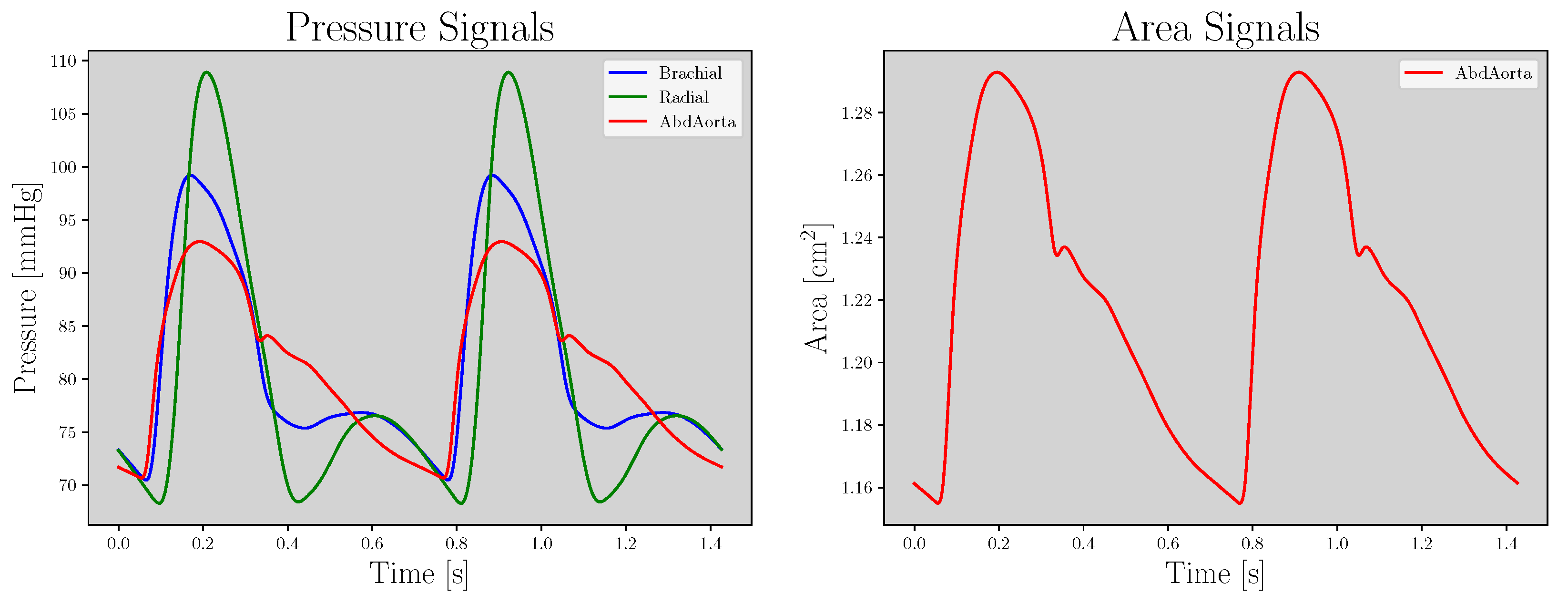
2.1. Dataset
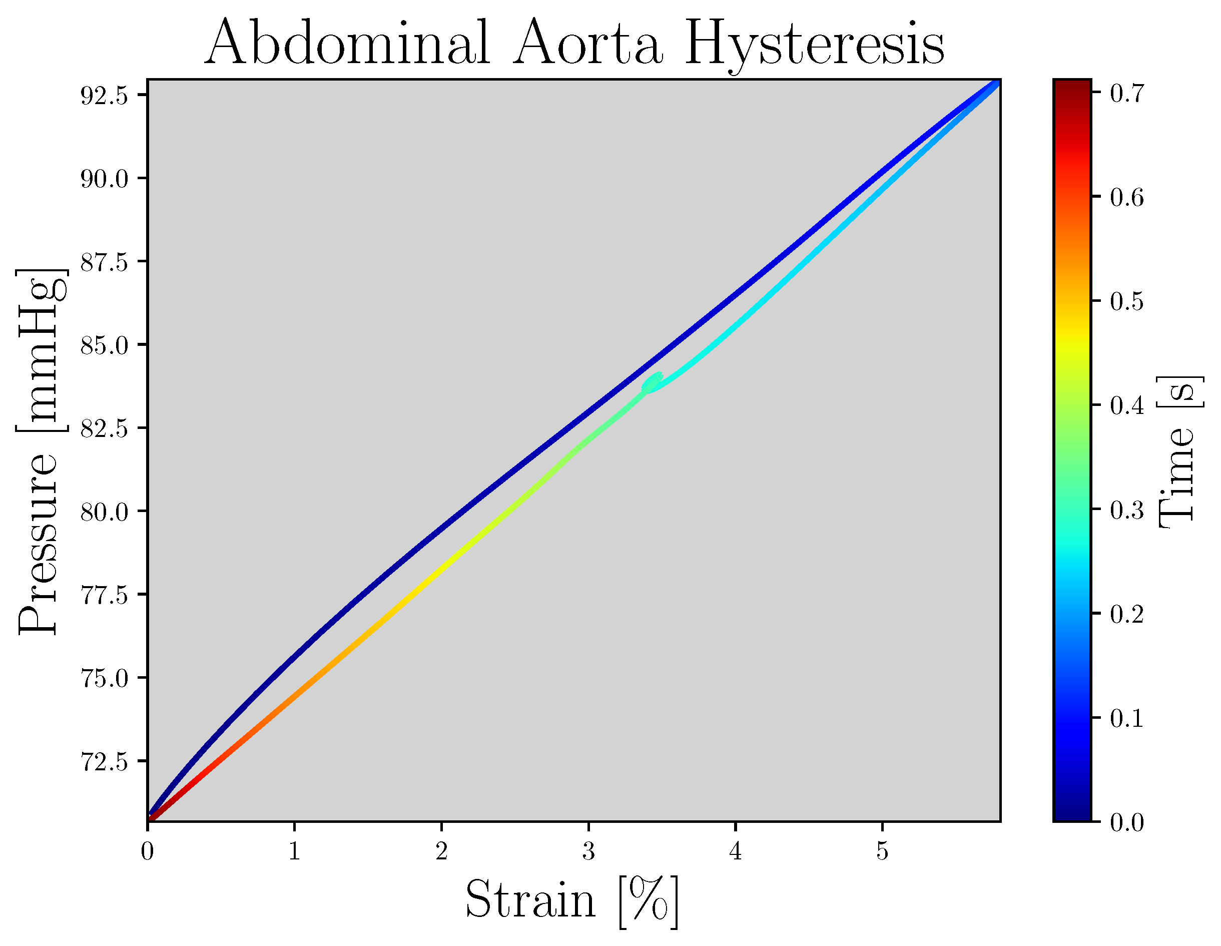
2.2. Pressure–Strain Elastic Modulus
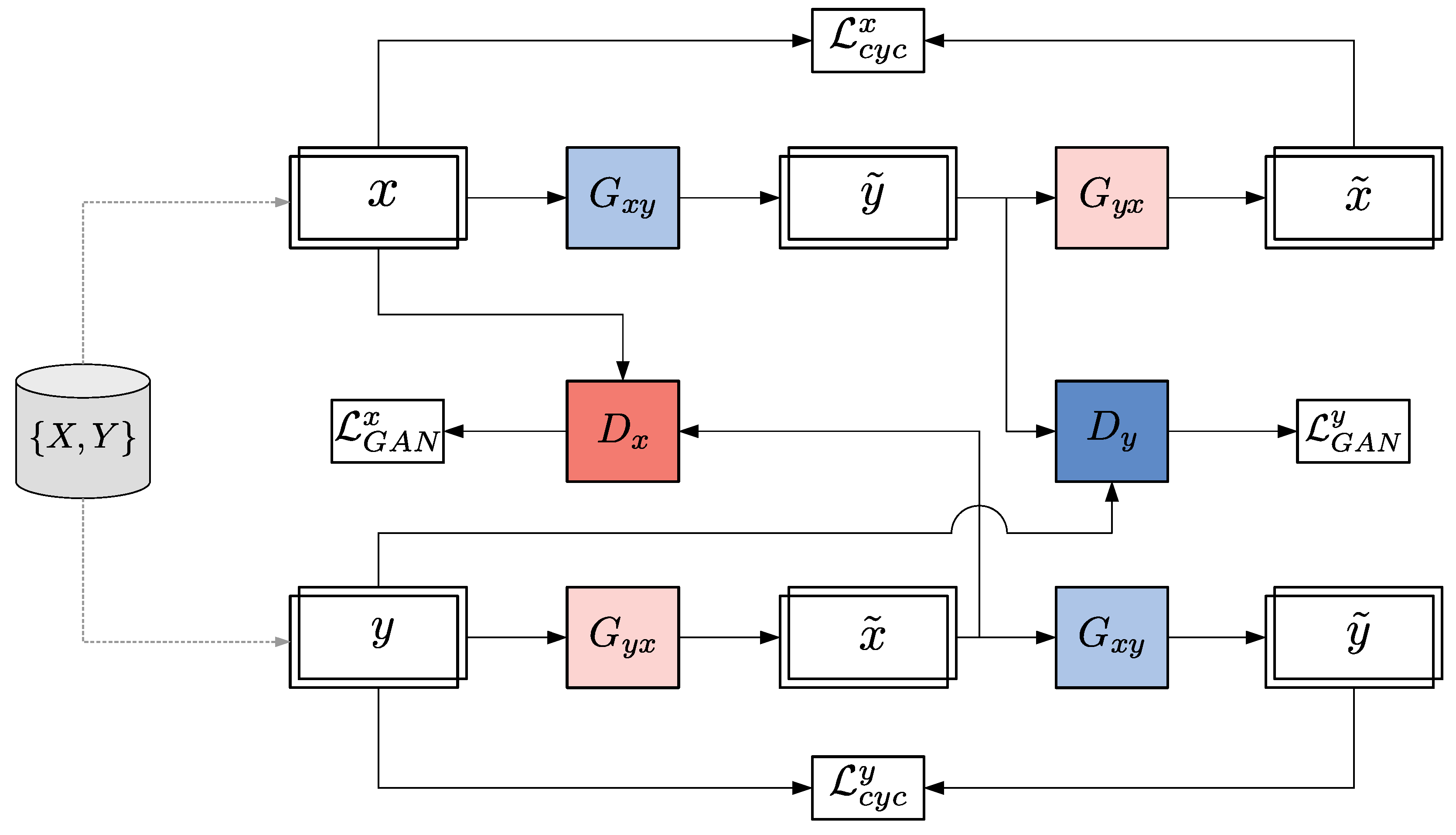
2.3. CycleGAN Model
2.3.1. General Architecture
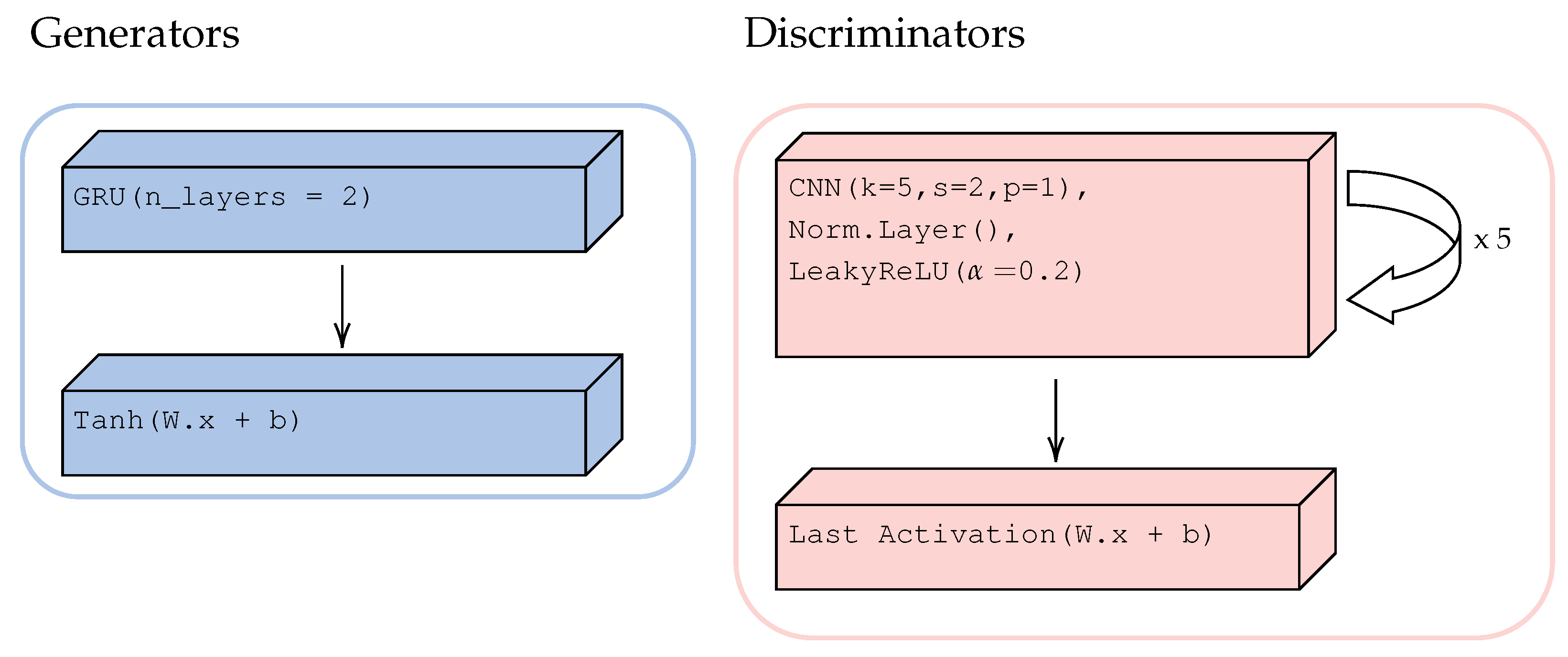
2.3.2. Architecture of Generators and Discriminators
2.3.3. Loss Functions
- where LSGAN and WGAN-GP measure the Pearson divergence and the Wasserstein distance, respectively. For the sake of simplicity, only the case where (the second term in Equation (5)) is written, because is defined analogously by replacing the X with the Y domain and vice versa. The objective for considering LSGAN is defined as follows:
2.3.4. Hyperparameters and Experimental Settings
2.4. Evaluation
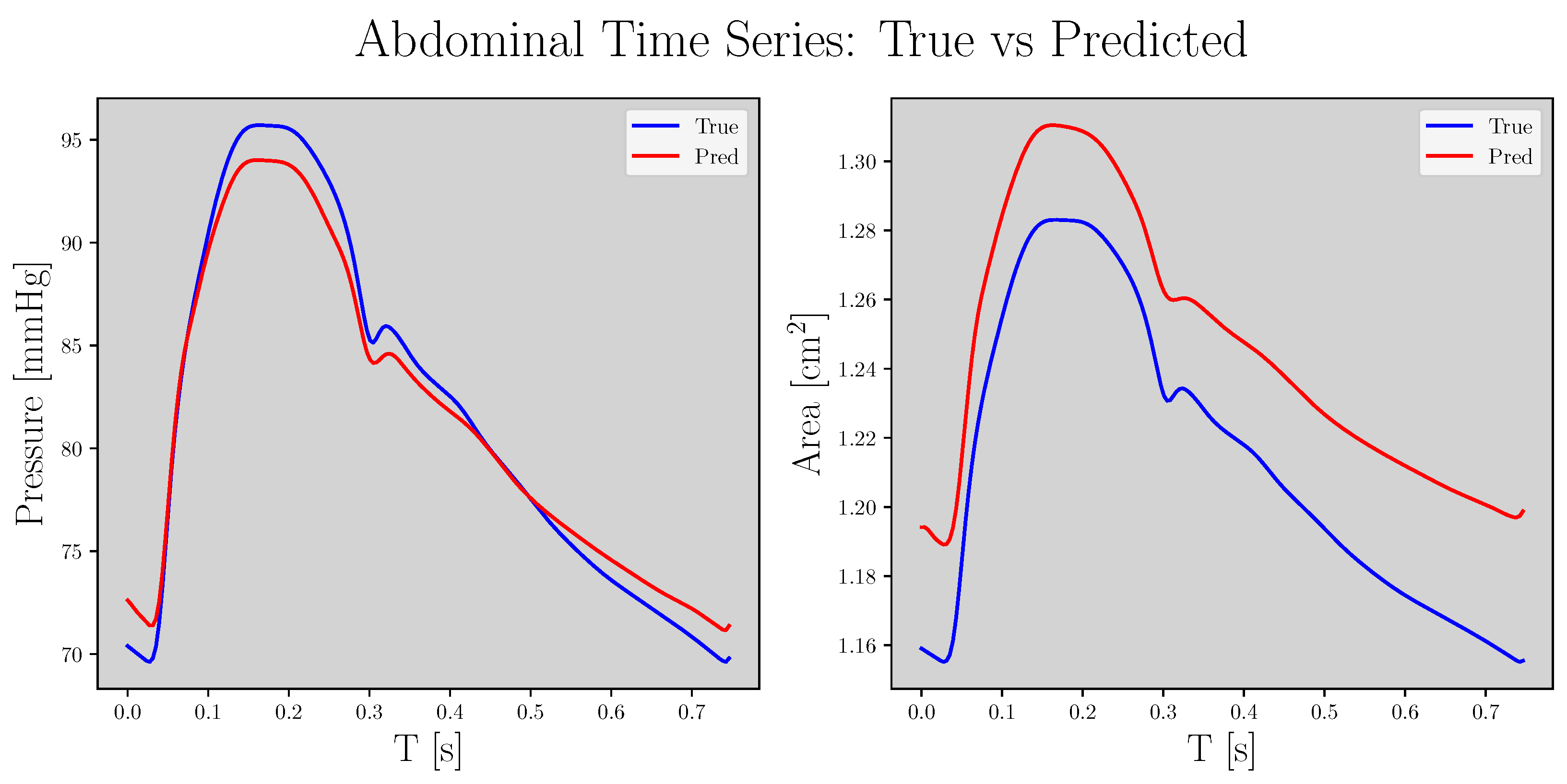
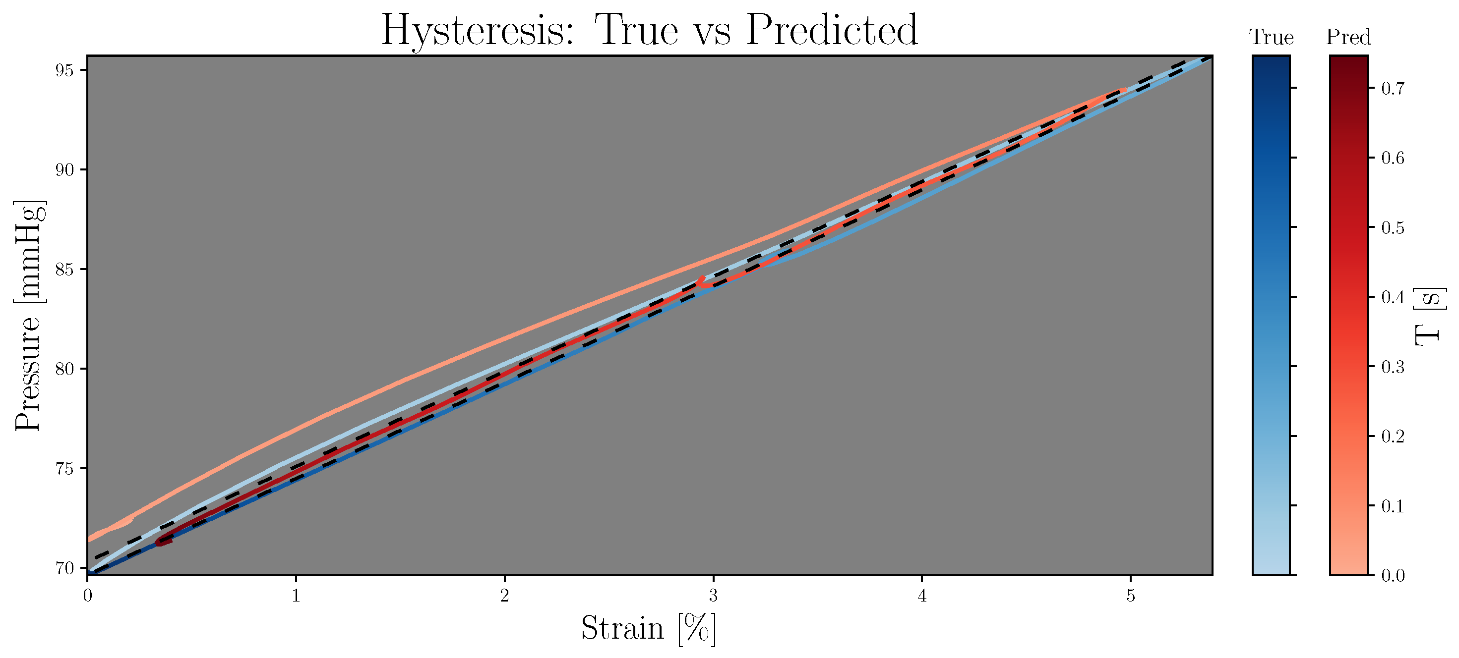
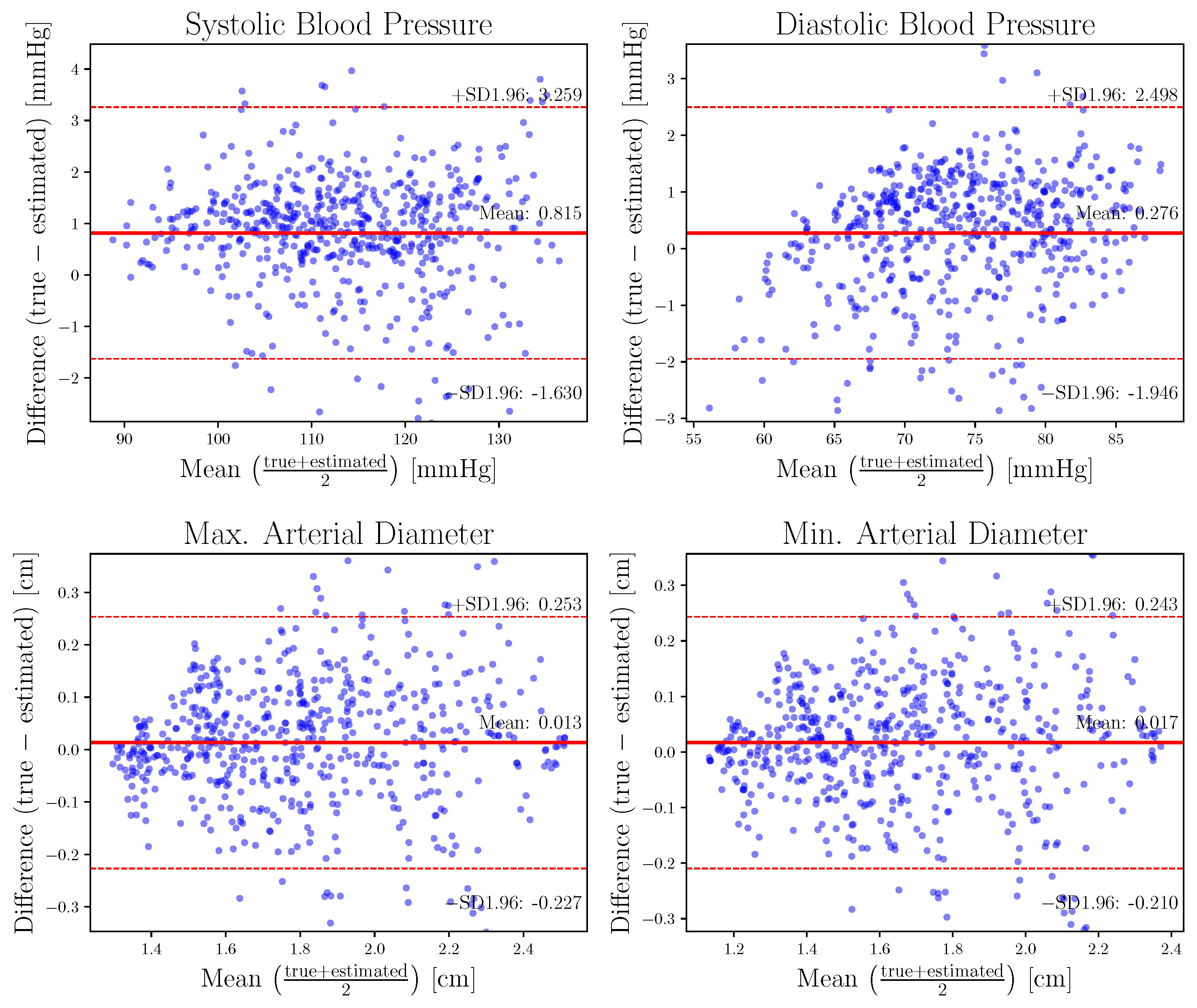
3. Results
4. Discussion
5. Conclusions
Supplementary Materials
Author Contributions
Funding
Data Availability Statement
Conflicts of Interest
Abbreviations
| BP | blood pressure |
| CNN | convolutional neural network |
| CV | cardiovascular |
| CVD | cardiovascular disease |
| DBP | diastolic blood pressure |
| E | elastic module |
| EP- | pressure–strain elastic modulus |
| GAN | generative adversarial network |
| GRU | gated recurrent unit |
| LOA | limit of agreement |
| LR | learning rate |
| LSGAN | least-square GAN |
| MAPE | mean absolute percentage error |
| ME | mean error |
| ML | machine learning |
| NN | neural network |
| P-D | pressure–diameter |
| PPG | photoplethysmography |
| PW | pulse wave |
| PWV | pulse wave velocity |
| RMSE | root mean squared error |
| SBP | systolic blood pressure |
| SVM | support vector machine |
| WGAN-GP | Wasserstein GAN with gradient penalty |
Appendix A

| Experiment | |||||
|---|---|---|---|---|---|
| LSGAN | 128 | 8 | 1 | 5 | A |
| WGAN-GP | 64 | 6 | 15 | 25 | B |
| LSGAN | 64 | 6 | 1 | 15 | C |
| 64 | 6 | 1 | 25 | D | |
| 64 | 6 | 1 | 5 | E | |
| WGAN-GP | 128 | 8 | 15 | 5 | F |
| 64 | 6 | 10 | 5 | G | |
| 64 | 6 | 15 | 15 | H | |
| 64 | 6 | 15 | 5 | I | |
| 64 | 6 | 50 | 15 | J | |
| 64 | 6 | 50 | 25 | K |
| Experiment | Pressure [mmHg] | Area [cm2] | [mmHg/%] | ||
|---|---|---|---|---|---|
| RMSE | RMSE | ME | MAPE | ||
| LSGAN | A | 0.8 ± 0.4 | 0.1 ± 0.1 | 13.1 ± 56.5 | 6.5 ± 5.1 |
| WGAN-GP | B | 1.7 ± 0.8 | 0.2 ± 0.2 | 70.6 ± 216.0 | 28.6 ± 19.3 |
| LSGAN | C | 4.4 ± 1.2 | 0.2 ± 0.1 | 229.3 ± 304.6 | 45.0 ± 25.7 |
| D | 27.1 ± 6.3 | 0.2 ± 0.1 | 654.2 ± 265.4 | 137.5 ± 14.6 | |
| E | 5.8 ± 3.3 | 0.3 ± 0.2 | 18.0 ± 137.7 | 17.3 ± 13.1 | |
| WGAN-GP | F | 2.7 ± 1.7 | 0.4 ± 0.2 | 3.1 ± 349.1 | 59.7 ± 54.4 |
| G | 3.8 ± 1.8 | 0.2 ± 0.1 | 84.3 ± 201.0 | 28.7 ± 19.5 | |
| H | 1.5 ± 0.7 | 0.4 ± 0.3 | 104.8 ± 222.3 | 28.7 ± 22.7 | |
| I | 3.4 ± 2.1 | 0.3 ± 0.2 | 10.9 ± 273.3 | 39.3 ± 31.9 | |
| J | 1.6 ± 0.7 | 0.4 ± 0.2 | 12.7 ± 300.1 | 48.2 ± 47.0 | |
| K | 2.0 ± 0.8 | 0.2 ± 0.2 | 68.4 ± 242.7 | 32.9 ± 23.6 | |
References
- World Health Organization. Cardiovascular Diseases (CVDs). 2021. Available online: https://www.who.int/news-room/fact-sheets/detail/cardiovascular-diseases-(cvds) (accessed on 19 May 2022).
- Salvi, P. Pulse Waves: How Vascular Hemodynamics Affects Blood Pressure, 2nd ed.; Springer International Publishing: Cham, Switzerland, 2017. [Google Scholar] [CrossRef]
- Armentano, R.L.; Barra, J.G.; Levenson, J.; Simon, A.; Pichel, R.H. Arterial Wall Mechanics in Conscious Dogs. Circ. Res. 1995, 76, 468–478. [Google Scholar] [CrossRef] [PubMed]
- Cymberknop, L.J.; Gabaldon Castillo, F.; Armentano, R.L. Beat to Beat Modulation of Arterial Pulse Wave Velocity Induced by Vascular Smooth Muscle Tone. In Proceedings of the 2019 41st Annual International Conference of the IEEE Engineering in Medicine and Biology Society (EMBC), Berlin, Germany, 23–27 July 2019; Volume 2019, pp. 5030–5033. [Google Scholar] [CrossRef]
- Alty, S.R.; Angarita-Jaimes, N.; Millasseau, S.C.; Chowienczyk, P.J. Predicting Arterial Stiffness From the Digital Volume Pulse Waveform. IEEE Trans. Biomed. Eng. 2007, 54, 2268–2275. [Google Scholar] [CrossRef] [PubMed]
- Tavallali, P.; Razavi, M.; Pahlevan, N.M. Artificial Intelligence Estimation of Carotid-Femoral Pulse Wave Velocity Using Carotid Waveform. Sci. Rep. 2018, 8, 1014. [Google Scholar] [CrossRef] [PubMed]
- Jin, W.; Chowienczyk, P.; Alastruey, J. Estimating Pulse Wave Velocity from the Radial Pressure Wave Using Machine Learning Algorithms. PLoS ONE 2021, 16, e0245026. [Google Scholar] [CrossRef]
- Mildenhall, B.; Srinivasan, P.P.; Tancik, M.; Barron, J.T.; Ramamoorthi, R.; Ng, R. NeRF: Representing Scenes as Neural Radiance Fields for View Synthesis. arXiv 2020, arXiv:cs/2003.08934. [Google Scholar] [CrossRef]
- Charlton, P.H.; Mariscal Harana, J.; Vennin, S.; Li, Y.; Chowienczyk, P.; Alastruey, J. Modeling Arterial Pulse Waves in Healthy Aging: A Database for in Silico Evaluation of Hemodynamics and Pulse Wave Indexes. Am. J. Physiol.-Heart Circ. Physiol. 2019, 317, H1062–H1085. [Google Scholar] [CrossRef]
- Xiao, H.; Tan, I.; Butlin, M.; Li, D.; Avolio, A.P. Arterial Viscoelasticity: Role in the Dependency of Pulse Wave Velocity on Heart Rate in Conduit Arteries. Am. J. Physiol.-Heart Circ. Physiol. 2017, 312, H1185–H1194. [Google Scholar] [CrossRef]
- Willemet, M.; Vennin, S.; Alastruey, J. Computational Assessment of Hemodynamics-Based Diagnostic Tools Using a Database of Virtual Subjects: Application to Three Case Studies. J. Biomech. 2016, 49, 3908–3914. [Google Scholar] [CrossRef] [Green Version]
- Alastruey, J. Numerical Assessment of Time-Domain Methods for the Estimation of Local Arterial Pulse Wave Speed. J. Biomech. 2011, 44, 885–891. [Google Scholar] [CrossRef]
- Bikia, V.; Papaioannou, T.G.; Pagoulatou, S.; Rovas, G.; Oikonomou, E.; Siasos, G.; Tousoulis, D.; Stergiopulos, N. Noninvasive Estimation of Aortic Hemodynamics and Cardiac Contractility Using Machine Learning. Sci. Rep. 2020, 10, 15015. [Google Scholar] [CrossRef]
- Ipar, E.; Aguirre, N.A.; Cymberknop, L.J.; Armentano, R.L. Blood Pressure Morphology as a Fingerprint of Cardiovascular Health: A Machine Learning Based Approach. In Proceedings of the Applied Informatics; Florez, H., Pollo-Cattaneo, M.F., Eds.; Communications in Computer and Information Science; Springer International Publishing: Cham, Switzerland, 2021; pp. 253–265. [Google Scholar] [CrossRef]
- Xiao, H.; Liu, D.; Avolio, A.P.; Chen, K.; Li, D.; Hu, B.; Butlin, M. Estimation of Cardiac Stroke Volume from Radial Pulse Waveform by Artificial Neural Network. Comput. Methods Programs Biomed. 2022, 218, 106738. [Google Scholar] [CrossRef]
- Armentano, R.L.; Cymberknop, L.J.; Legnani, W.; Pessana, F.M.; Craiem, D.; Graf, S.; Barra, J.G. Arterial Pressure Fractality Is Highly Dependent on Wave Reflection. In Proceedings of the 2013 35th Annual International Conference of the IEEE Engineering in Medicine and Biology Society (EMBC), Osaka, Japan, 3–7 July 2013; pp. 1960–1963. [Google Scholar] [CrossRef]
- Zhu, J.Y.; Park, T.; Isola, P.; Efros, A.A. Unpaired Image-to-Image Translation Using Cycle-Consistent Adversarial Networks. arXiv 2020, arXiv:1703.10593. [Google Scholar]
- Mao, X.; Li, Q.; Xie, H.; Lau, R.Y.K.; Wang, Z.; Smolley, S.P. Least Squares Generative Adversarial Networks. arXiv 2017, arXiv:1611.04076. [Google Scholar]
- Gulrajani, I.; Ahmed, F.; Arjovsky, M.; Dumoulin, V.; Courville, A. Improved Training of Wasserstein GANs. arXiv 2017, arXiv:1704.00028. [Google Scholar]
- Kingma, D.P.; Ba, J. Adam: A Method for Stochastic Optimization. arXiv 2017, arXiv:1412.6980. [Google Scholar]
- Arjovsky, M.; Chintala, S.; Bottou, L. Wasserstein GAN. arXiv 2017, arXiv:1701.07875. [Google Scholar]
- Stefanadis, C.; Stratos, C.; Vlachopoulos, C.; Marakas, S.; Boudoulas, H.; Kallikazaros, I.; Tsiamis, E.; Toutouzas, K.; Sioros, L.; Toutouzas, P. Pressure-Diameter Relation of the Human Aorta. Circulation 1995, 92, 2210–2219. [Google Scholar] [CrossRef]
- McEniery Carmel, M.; Yasmin, N.; McDonnell, B.; Munnery, M.; Wallace Sharon, M.; Rowe Chloe, V.; Cockcroft John, R.; Wilkinson Ian, B. Central Pressure: Variability and Impact of Cardiovascular Risk Factors. Hypertension 2008, 51, 1476–1482. [Google Scholar] [CrossRef]
- Agabiti-Rosei, E.; Mancia, G.; O’Rourke Michael, F.; Roman Mary, J.; Safar Michel, E.; Smulyan, H.; Wang, J.-G.; Wilkinson Ian, B.; Williams, B.; Vlachopoulos, C. Central Blood Pressure Measurements and Antihypertensive Therapy. Hypertension 2007, 50, 154–160. [Google Scholar] [CrossRef]
- Sadrawi, M.; Lin, Y.T.; Lin, C.H.; Mathunjwa, B.; Fan, S.Z.; Abbod, M.F.; Shieh, J.S. Genetic Deep Convolutional Autoencoder Applied for Generative Continuous Arterial Blood Pressure via Photoplethysmography. Sensors 2020, 20, 3829. [Google Scholar] [CrossRef]
- Sideris, C.; Kalantarian, H.; Nemati, E.; Sarrafzadeh, M. Building Continuous Arterial Blood Pressure Prediction Models Using Recurrent Networks. In Proceedings of the 2016 IEEE International Conference on Smart Computing (SMARTCOMP), St. Louis, MO, USA, 18–20 May 2016; pp. 1–5. [Google Scholar] [CrossRef]
- Aguirre, N.; Grall-Maës, E.; Cymberknop, L.J.; Armentano, R.L. Blood Pressure Morphology Assessment from Photoplethysmogram and Demographic Information Using Deep Learning with Attention Mechanism. Sensors 2021, 21, 2167. [Google Scholar] [CrossRef] [PubMed]
- Brophy, E.; De Vos, M.; Boylan, G.; Ward, T. Estimation of Continuous Blood Pressure from PPG via a Federated Learning Approach. arXiv 2021, arXiv:2102.12245. [Google Scholar] [CrossRef]
- Armentano, R.L.; Cymberknop, L.J. Quantitative Vascular Evaluation: From Laboratory Experiments to Point-of-Care Patient (Clinical Approach). Curr. Hypertens. Rev. 2018, 14, 86–94. [Google Scholar] [CrossRef]
- Armentano, R.L.; Cymberknop, L.J. Quantitative Vascular Evaluation: From Laboratory Experiments to Point-of-Care Patient (Experimental Approach). Curr. Hypertens. Rev. 2018, 14, 76–85. [Google Scholar] [CrossRef] [PubMed]
- Liu, Y.; Dang, C.; Garcia, M.; Gregersen, H.; Kassab, G.S. Surrounding Tissues Affect the Passive Mechanics of the Vessel Wall: Theory and Experiment. Am. J. Physiol.-Heart Circ. Physiol. 2007, 293, H3290–H3300. [Google Scholar] [CrossRef] [PubMed]


| [LSGAN, WGAN-GP] | [64, 128] | [6, 8] | [5, 15, 25] | [5, 15, 25] |
| Experiment | Pressure [mmHg] | Area [cm2] | [mmHg/%] | ||
|---|---|---|---|---|---|
| RMSE | RMSE | ME | MAPE | ||
| LSGAN | A | 0.8 ± 0.4 | 0.1 ± 0.1 | 13.1 ± 56.5 | 6.5 ± 5.1 |
| WGAN-GP | B | 1.7 ± 0.8 | 0.2 ± 0.2 | 70.6 ± 216.0 | 28.6 ± 19.3 |
| Experiment | Pressure [mmHg] | Area [cm2] | [mmHg/%] | ||
|---|---|---|---|---|---|
| RMSE | RMSE | ME | MAPE | ||
| LSGAN | A | 0.8 ± 0.4 | 0.1 ± 0.1 | 13.4 ± 51.5 | 6.2 ± 4.9 |
| WGAN-GP | B | 1.8 ± 0.9 | 0.2 ± 0.2 | 71.1 ± 209.3 | 28.3 ± 20.8 |
Disclaimer/Publisher’s Note: The statements, opinions and data contained in all publications are solely those of the individual author(s) and contributor(s) and not of MDPI and/or the editor(s). MDPI and/or the editor(s) disclaim responsibility for any injury to people or property resulting from any ideas, methods, instructions or products referred to in the content. |
© 2023 by the authors. Licensee MDPI, Basel, Switzerland. This article is an open access article distributed under the terms and conditions of the Creative Commons Attribution (CC BY) license (https://creativecommons.org/licenses/by/4.0/).
Share and Cite
Aguirre, N.; Cymberknop, L.J.; Grall-Maës, E.; Ipar, E.; Armentano, R.L. Central Arterial Dynamic Evaluation from Peripheral Blood Pressure Waveforms Using CycleGAN: An In Silico Approach. Sensors 2023, 23, 1559. https://doi.org/10.3390/s23031559
Aguirre N, Cymberknop LJ, Grall-Maës E, Ipar E, Armentano RL. Central Arterial Dynamic Evaluation from Peripheral Blood Pressure Waveforms Using CycleGAN: An In Silico Approach. Sensors. 2023; 23(3):1559. https://doi.org/10.3390/s23031559
Chicago/Turabian StyleAguirre, Nicolas, Leandro J. Cymberknop, Edith Grall-Maës, Eugenia Ipar, and Ricardo L. Armentano. 2023. "Central Arterial Dynamic Evaluation from Peripheral Blood Pressure Waveforms Using CycleGAN: An In Silico Approach" Sensors 23, no. 3: 1559. https://doi.org/10.3390/s23031559