1. Introduction
Magnetoencephalography (MEG) enables the non-invasive characterization of human brain function and thus provides unique insights into the neural substrates that underpin functions and dysfunctions processes in both research [
1,
2] and clinical [
3,
4] settings. Although SQUID-based MEG has a high spatial resolution (by minimizing the volume conduction effect and amplitude attenuation through skull conductivity), the technique has some inherent limitations. Firstly, liquid helium (He) must be used to reach sufficiently low temperatures. Secondly, the cryogenic constraint limits the flexibility of sensor configurations, and a SQUID-based system cannot be adjusted to suit different individual head shapes and sizes (e.g., as encountered with children and infants) [
5]. Baby MEG systems have been developed [
6], however they are not widely available. Thirdly, systems tailored to a baby’s head size are still limited by their rigid sensor configuration and the thermal insulation required by the cryogenic sensors; a distance of at least about three cm between the sensors and the subject’s scalp is typically required. Reducing this distance as much as possible is mandatory as the amplitude of the magnetic field decreases with the cube of the sensor-scalp distance
r (i.e., vs.
). Fourthly, head movements inside the fixed cap (support + sensors) also impede the accuracy of source localization, since the sensors will not always be recording the same regions of the brain. This might be a limitation in a patient who makes uncontrolled movements (e.g., a patient with Parkinson’s disease) [
5] and in children and infants. Lastly, the size of SQUID-based MEG systems also necessarily requires the use of large, costly, heavy magnetically shielded rooms (MSRs) and this imposes strong infrastructural constraints on buildings, in which these devices are installed. Overall, the ability to capture brain function via a “wearable” scanning device (i.e., one that can be adapted to fit any individual subject’s head shape and size, and that enables free movement during recording) is of major interest.
Currently, electroencephalography (EEG) systems are the most widely used wearable neuroimaging devices. EEG instrumentation is lightweight and flexible and can be adapted to any head size—making it usable in almost any experimental setting. However, EEG has significant technological drawbacks, relative to MEG. The head’s inhomogeneous conductivity profile reduces the amplitude of the electrical potentials and spatially blurs the signal on the scalp surface [
7,
8]. These factors place a practical limit on the spatial resolution of EEG [
9]. Accordingly, wearable MEG (giving a higher spatial resolution) is a compelling prospect.
The recent development of new MEG sensors (such as alkali optically pumped magnetometers [OPMs] [
10]) has now produced the sensitivity gains required for the detection of neuromagnetic fields. OPMs working in the spin-exchange relaxation-free (SERF) regime demonstrated a sensitivity of 5 fT/
with a 6 × 6
footprint [
11]. Mhaskar and colleagues [
12] created a smaller chip-scale microfabricated OPM with a volume of around 1
and a sensitivity of more than 20 fT/
. An OPM with a volume of 2 × 2 × 5
and a sensitivity of 10 fT/
was demonstrated by Shah and Wakai [
13]. The advantages of being able to place these new MEG imaging sensors closer to the brain have already been demonstrated in adults [
14,
15]. By eliminating the need for liquid He, the drastic reduction in the system’s size and brain-to-sensor distance has enabled the implementation of a wearable MEG headset [
16]. Removing the Dewar containing liquid, He also reduces the size of the MEG system, and thus, the cost of the MSR. However, these alkali OPMs suffer from a small dynamic range and a narrow bandwidth. The small dynamic range requires perfect control of the ambient magnetic field inside the MSR, by using field-nulling coil systems [
5,
17,
18] to limit the saturation of these sensors as soon as the magnetic field offset exceeds 5 nT. Limiting the bandwidth to 100 Hz prevents the recording of fast brain oscillations, such as high gamma band activity. Furthermore, alkali OPMs have to be heated to over 100 °C. Dissipation of this heat requires the sensor to be moved a few millimeters away from the scalp, which impedes the recording of brain activity. These alkali OPMs are also limited to one or two axes measurement of the brain’s magnetic field.
Some of the limitations of alkali OPMs can be overcome by using OPMs based on helium four atoms [
19] in their
F = one metastable level, which can be significantly populated by using a low-intensity radio-frequency discharge of only a few milliwatts. Since helium is a gas at room temperature, these
4He OPMs can be operated at room temperature (i.e., with no need for heating or cooling) and can be placed in direct contact with the subject’s scalp (thus optimally reducing the brain-sensor distance). They have a large dynamic range (up to 200 nT) and a broad bandwidth (ranging from direct current to two kHz); these features enable the full spectrum of normal and pathological brain activities to be recorded. Furthermore,
4He OPMs operate more easily in a noisier magnetic environment. These devices provide exhaustive, three-axis measurements of the brain’s magnetic field thanks to two orthogonal rotating RF fields at different frequencies to record the double parametric resonance of He atoms. The concept of MEG recording with these
4He OPMs has been proved [
20]. The amplitude of brain responses is higher for
4He OPMs than for SQUIDs, thanks to the sensor’s proximity to the scalp. Since the proof-of-concept study, the sensitivity of
4He OPM systems has increased five-fold. A detailed technical description of
4He OPMs is reported in [
21,
22].
The primary objective of the present study was to assess the added value of a 4He OPM, relative to SQUIDs and alkali OPMs. To this end, a 4He OPM sensor array’s performance variables were modeled and compared with those obtained for an equivalent SQUID MEG array and a state-of-the-art alkali OPM array. The study’s secondary objective was to assess the added value of a 4He OPM sensor as a function of the subject’s age. To this end, the same variables were computed for the geometries of 12 healthy subjects, including adults, children, and infants. For SQUID MEG simulations, two different configurations were used: (i) a head-sized SQUID array (as used in a baby MEG system—the optimal set-up, yet one which is only available in a few centers worldwide); and (ii) a head position translated along the vertical axis, as more usually performed with standard SQUID MEG systems (where the top of the baby’s head is placed close to the MEG helmet). The metrics derived from forward and inverse models included the signal power, information capacity, localization accuracy, and the dependency of the respective MEG and OPM signal magnitudes on the orientation of a current dipole.
2. Materials and Methods
2.1. Head Models
T1-weighted MRI datasets were obtained from 12 healthy subjects aged from one month to the adult age. In each case, the brain, skull and scalp compartments were segmented using FreeSurfer software [
23]. A surface mesh of the cortical gray-white matter border was created with roughly 300,000 vertices, which was subsequently downsampled to 15,002 vertices. Skull and scalp surfaces were triangulated and decimated to obtain meshes with 1922 vertices each. The boundary element method (BEM [
24]) was used to create the head model. We assumed that the brain:skull:scalp conductivity ratio was 1:0.0125:1 [
25].
2.2. Source Space for the Cortex Surface and the Brain Volume
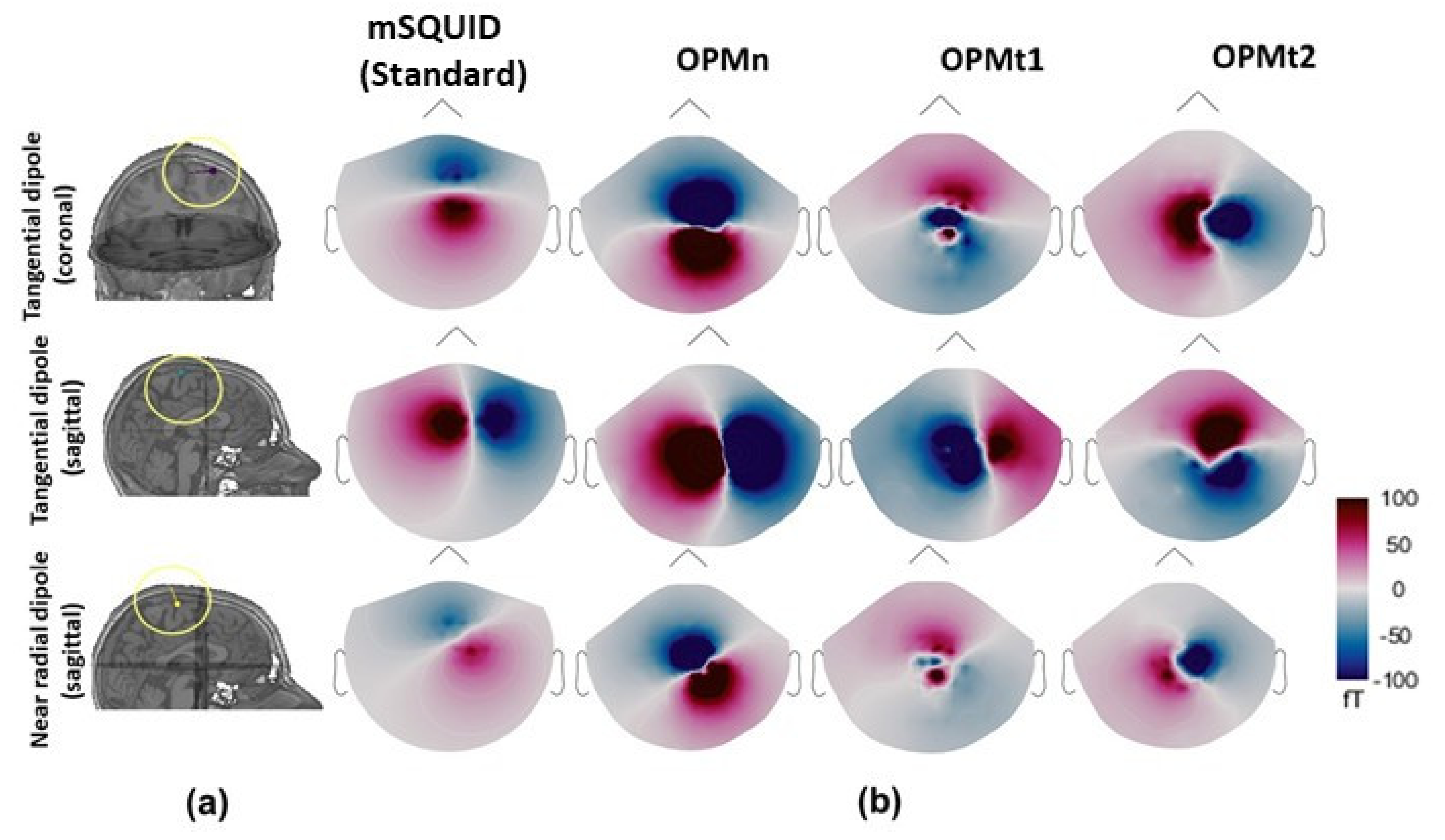
First, 2D topographic maps related to a single dipole simulated over the somatosensory area (the post central gyrus, hand area) with various orientations (one near-radial and two tangential) were computed, in order to characterize the magnetic field mapping along the 4He OPM’s three measurement axes for various dipolar brain source orientations. To enable more flexible simulation of the sources in various dimensions (such as depth and orientation), the source space was built within the brain volume. We used a source grid with 12,321 isotropic points within the brain volume and a grid resolution of 5 mm, and considered three orthogonal orientations per dipole on the x-, y-, and z-axes with unconstrained sources. The characterization of all the dipoles yielded a 12,321 × 3 matrix.
For all other simulations of the brain’s magnetic field and the computation of quantitative metrics, the source space was computed from the cortex surface mesh. Each vertex of the brain mesh was used to set a dipole source’s position, leading to a source space of 15,002 dipoles. The primary current distributions were considered to be at a depth of five mm in the cortical mantle.
2.3. Sensor Models
The sensor geometries are described in
Table 1. In total, four integration points were uniformly distributed throughout the volume of the
4He OPM sensor (a cube with a side length of 10 mm). The standard SQUID sensor model implemented in the Brainstorm software was used in the present study [
26]. The noise level was set to 40 fT
for
4He OPMs (as recommended in [
21]), and 5 fT
for SQUID magnetometers. With regard to the distances
d, the distance between the bottom part of the He gas cell and the scalp was considered as this was previously used in simulation work comparing alkali OPM [
15]. This distance was reasonably set to three mm, while the distance between SQUID and the scalp was set to 2 cm as previously used in [
15].
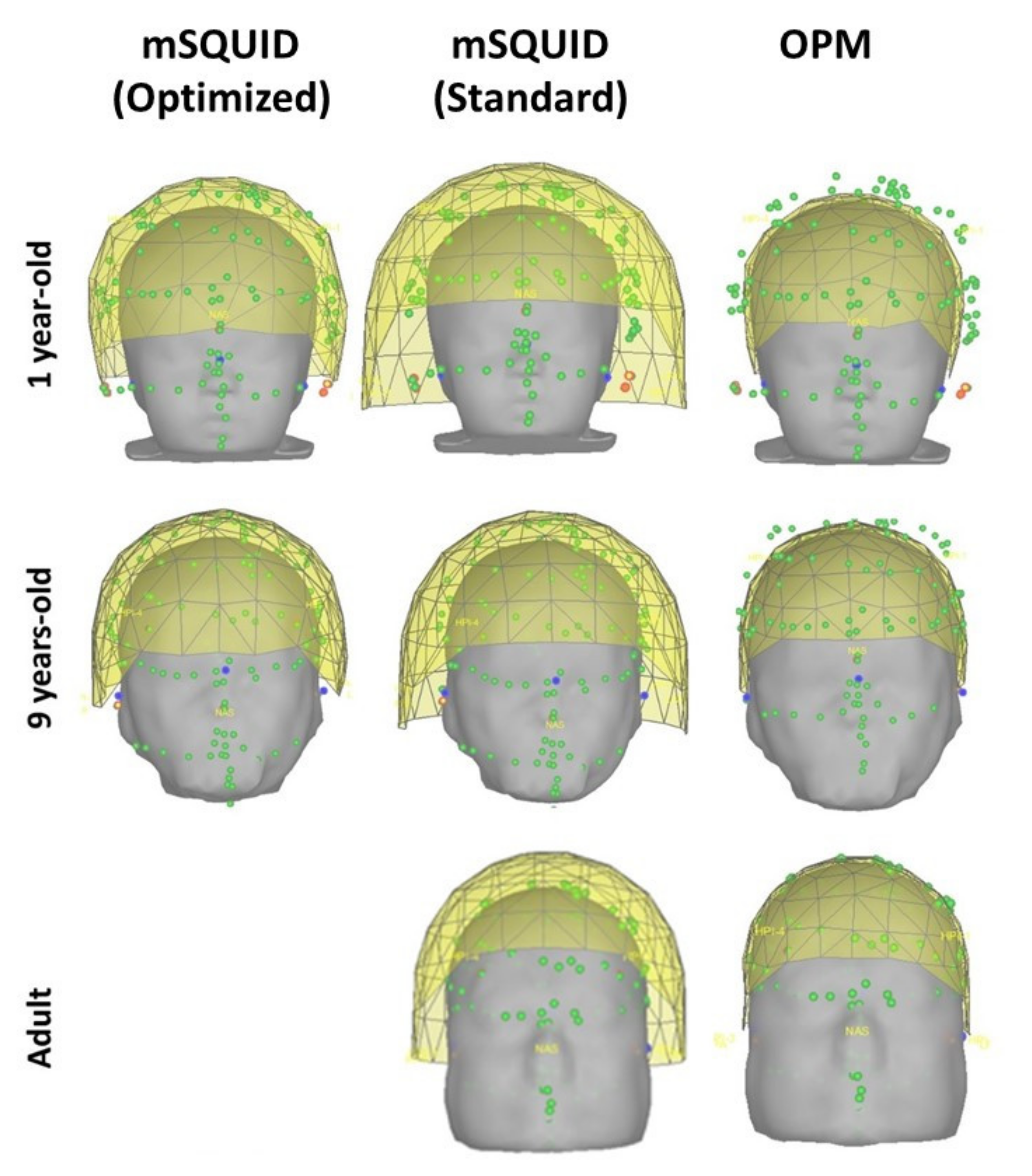
Two different configurations were used for SQUID MEG simulations in infants and children: (i) mSQUID (optimized), i.e., a baby MEG device for which the sensor-scalp distance (2 cm) is optimized all around the head, and (ii) mSQUID (standard), corresponding to a conventional SQUID MEG system, for which the top of the infant’s head was placed as close as possible to the helmet (around 2 cm from the sensors, along the z axis). Given the size of the adult head model, only the mSQUID (standard) configuration was considered (as usually performed during MEG examinations). The mSQUID sensor array still comprised N = 102 MEG magnetometers, which measured the magnetic field component that was nearly radial to the scalp’s surface.
Four OPM arrays were developed: three 102-sensor arrays that, respectively, measured the normal component of the magnetic field (OPMn), the first orthogonal tangential component (OPMt1) and the second orthogonal tangential component (OPMt2), and a 306-sensor combination of the three arrays that measured all field components (OPMa). The OPM sensor (the center of the 4He gas cell) was 3 mm away from the scalp.
Figure 1 represents the mSQUID (optimized), mSQUID (standard), and OPM sensor locations at different ages (an adult, a 9-year-old, and a 1-year-old). As mentioned above, only the mSQUID (standard) array was built for the adult.
2.4. The Forward Model
The forward problem occurs in computing, from a given electrical source (dipole), the electrical potential (or its related magnetic field obtained by integrating the total current using Biot–Savart law) at the sensors level.
MEG and OPM signals
S recorded from
M channels for
T time samples can be described as the weighted sum of the dipole signals
D .
where
L are the matrices containing the dipolar source lead fields that link the MEG or OPM signals in an array of
M sensors to the three components of a dipole moment vector at locations in the brain.
N is the additive noise. The forward matrix was computed using OpenMEEG software [
24].
2.5. The Inverse Model
Given the MEG signals
S(
t) and the gain matrix
L, the inverse problem consists of finding an estimate
D(
t) of the dipolar source parameters. We used minimum norm estimates [
25,
27] (based on the L2 norm) to regularize the problem and search for the solution with the minimum power. This form of estimator is best suited to distributed source models, in which the dipole activity is expected to span some portions of the cortical surface:
where
is the regularization parameter, and
C is the noise covariance matrix. The (symmetric) resolution matrix in this case is:
For linear estimators, the resolution matrix is a valuable tool for describing the spatial resolution [
28]. The relationship between the estimated and modeled current distributions is represented by the resolution matrix
R.
2.6. Evaluation Criteria
2.6.1. Signal Power
The
-norm of the source topography squared was used to define the topography power of the
ith source:
where
ti = (
C−1/2 L)
i is the whitened topography of the
ith source.
If we assume that all sensors in the array have an equal sensor noise variance σ2, the topography power is linearly proportional to the source’s signal-to-noise ratio.
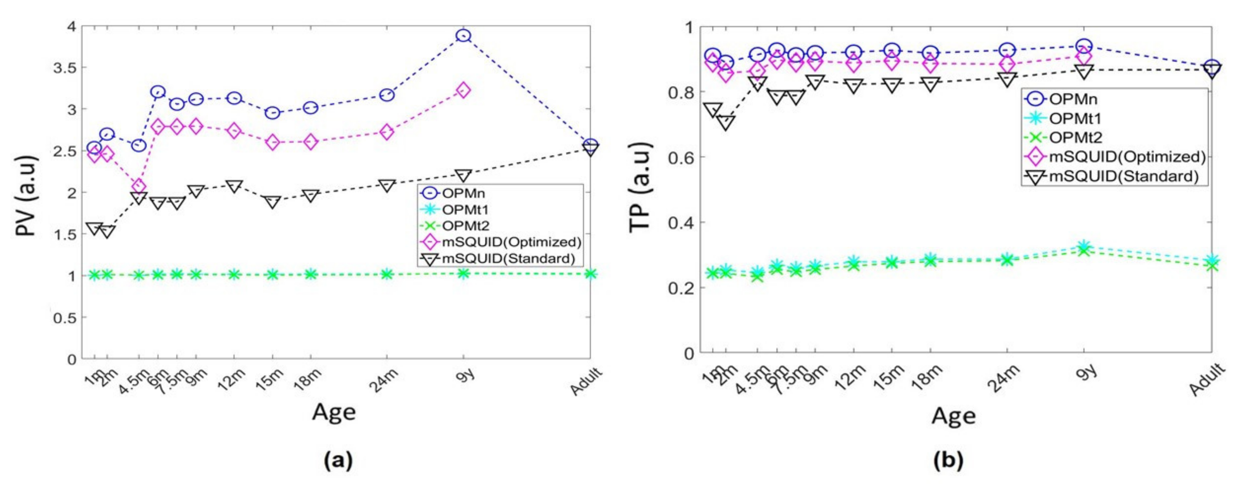
2.6.2. Contributions of Primary and Volume Currents
The contributions of the primary and volume currents to the total magnetic field were also investigated for the various sensor arrays. The ratio between the total current and the primary current was defined as TP:
where the
ith columns of the corresponding matrices
P V,
L are denoted by
,
and
,
P is the primary current,
V is the volume current, and
L =
P +
V is the total current.
By computing the ratio between the field components’ norms, we determined the relative overall magnitude of the primary and volume currents’ topographies for the various sensor arrays.
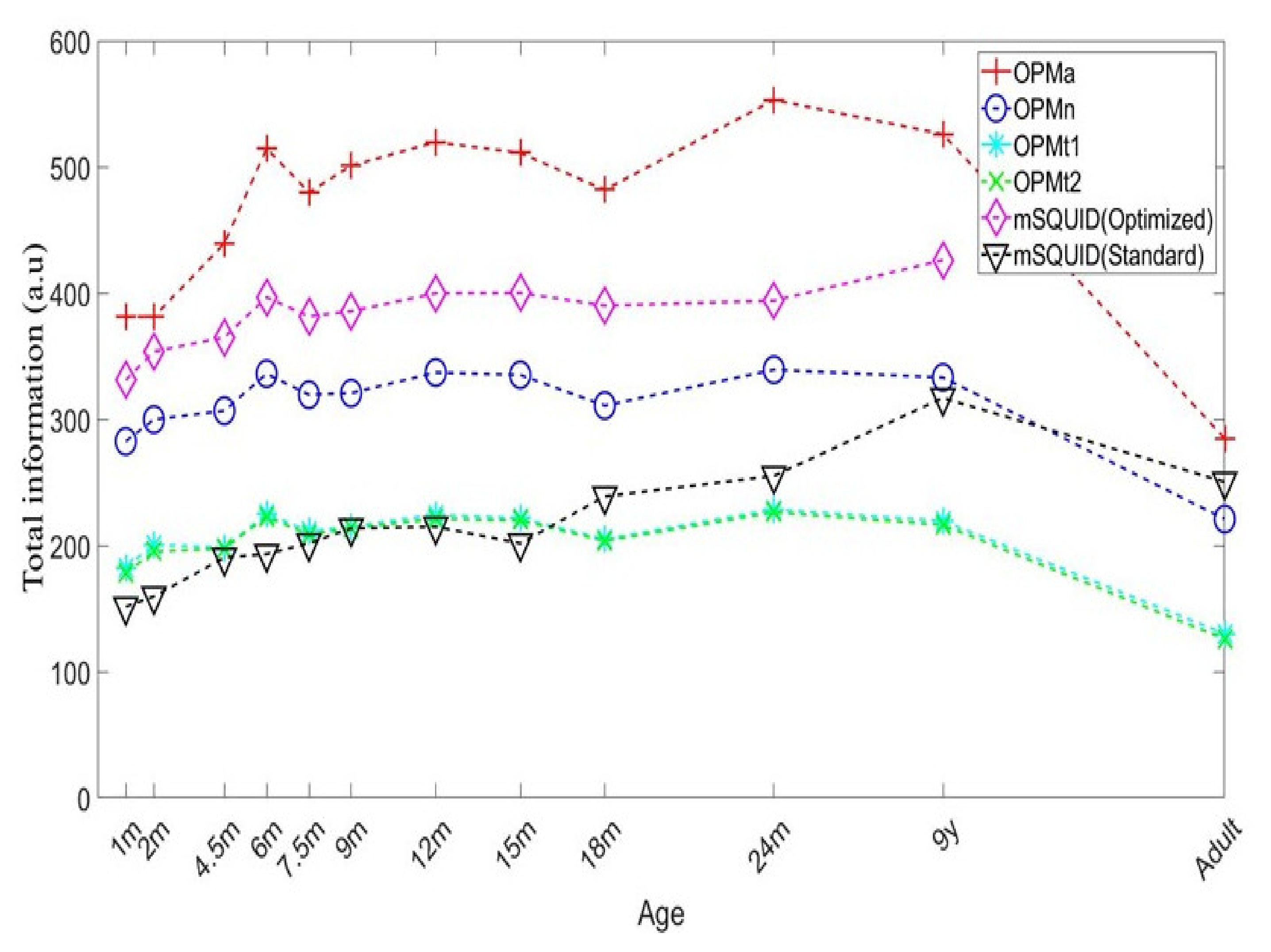
2.6.3. Total Information
(the information per sample of the multi-channel system) uses a single number to quantify all aspects of forward-model-based metrics [
29,
30], according to Shannon’s theory of communication [
31]:
where
is the signal-to-noise ratio of the
ith channel.
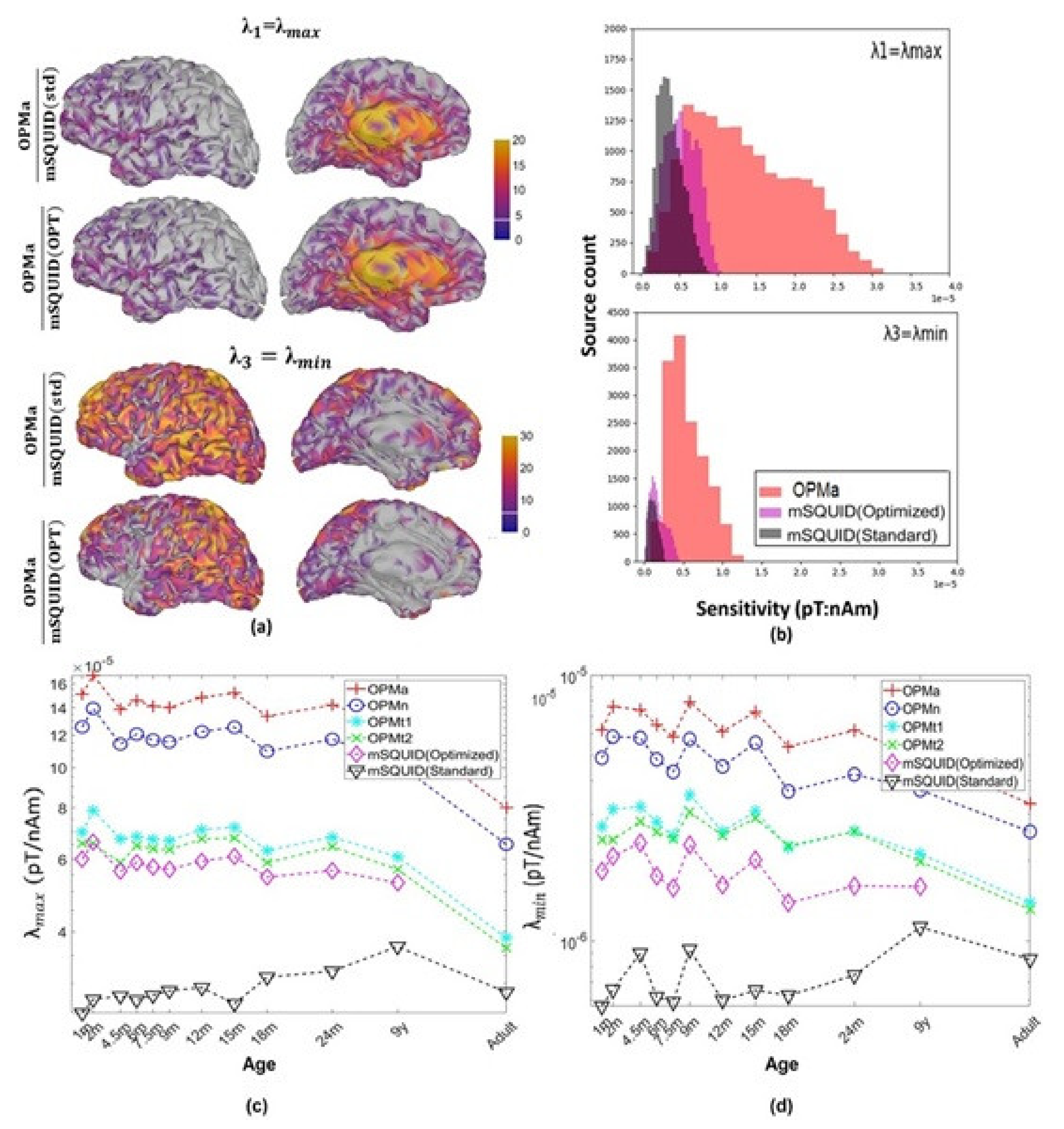
2.6.4. Singular Value Decomposition (SVD)
We generated the singular value decomposition of the
N × 3-dimensional dipolar gain matrix at each location indexed by
k = 1,…,
M to investigate the sensitivity of the mSQUID and OPM sensor arrays to sources with varied orientations [
32]:
where
and
are the left and right singular vectors, respectively, and the singular values are
,
and
. We denoted the largest and smallest singular values (corresponding to the dipole orientations, to which the mSQUID or OPM sensor array is the most and the least sensitive) as
=
and
=
, respectively.
corresponds to the tangentially oriented brain sources, to which MEG is most sensitive, whereas
, corresponds to the radially oriented brain sources, to which MEG is least sensitive.
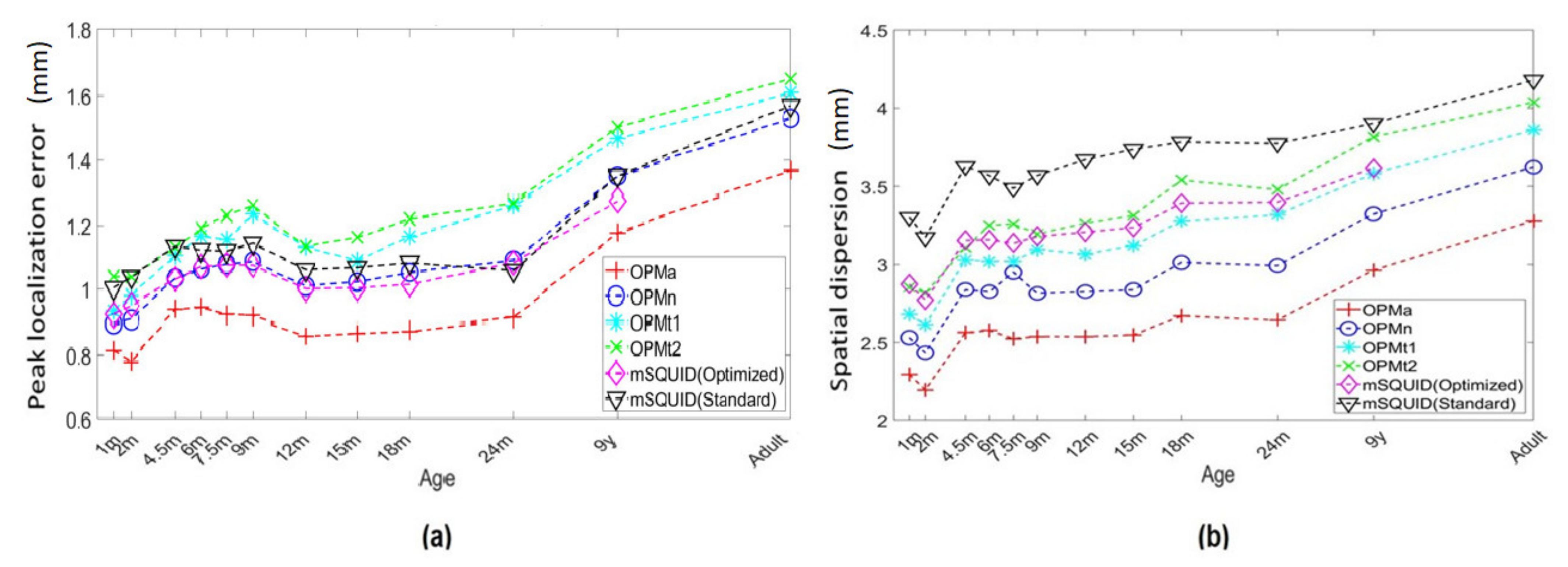
2.6.5. Dipole Localization Error
From the inverse model and the resolution matrix
R in particular, it is possible to compute various metrics to assess the performance of the source localization solution. Notably, the point-spread functions (PSFs) describe how an imaging system distorts a point source. The
ith column of the resolution matrix
R corresponds to the PSF for the source
i:
To assess the performance of the source imaging results obtained in our mSQUID and OPM data simulations, and to characterize the similarity between the original and the estimated source configurations, we used a PSF-derived metric: the dipole localization error (DLE) [
33]:
where
is the true location of the source
i and
is the location of the PSF peak for the source
i. Therefore, DLE quantifies the distance between the original and estimated source locations
2.6.6. Spatial Dispersion
This index (developed by Molins et al. [
34]) quantifies the spatial dispersion (SD) of the estimated source distribution around the true source location:
where
is the number of sources,
is the intensity of the source
j, and
is the location of the source
j.
2.7. Statistical Analysis
For each of the metrics, a t-test was used to determine whether or not there was a significant difference between 4He OPM and mSQUID (standard) or between 4He OPM and mSQUID (optimized) when this configuration was used for data simulation (children and infants). Pairwise, comparison with a t-test has been used as the simulated data for He OPM and SQUID were generated with the same headmodel for a given age.
Furthermore, a one-way analysis of variance (ANOVA) was also used to determine whether or not there was a significant age effect on the different metrics. When a significant effect of age was revealed, post hoc analyses were used to determine which specific ages differed from each other.
2.8. Data Simulation Procedure and Metric Computation for the Comparative Analysis
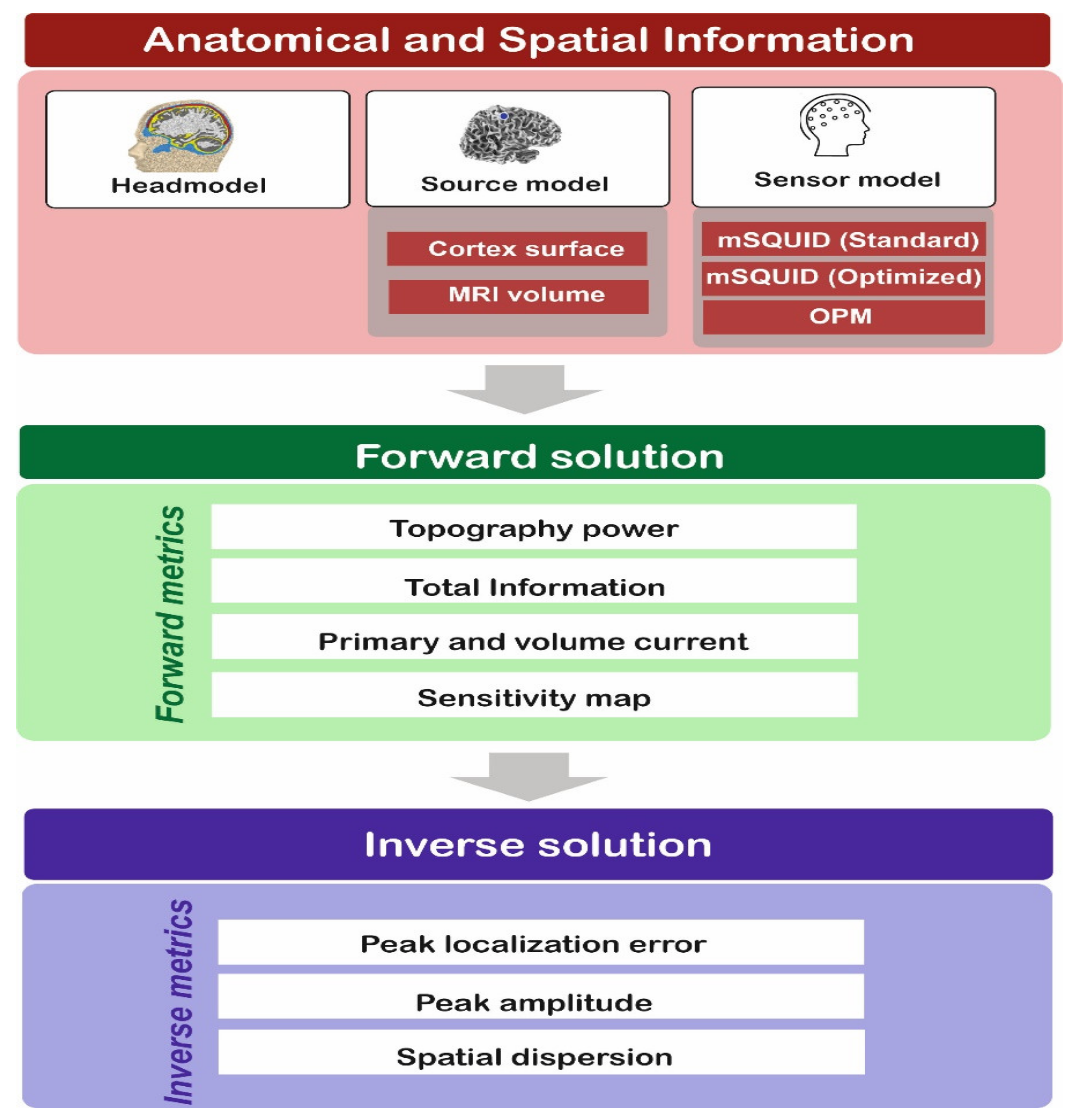
The steps in the comparative analysis are summarized in
Figure 2. In step 1, structural MR images were processed using the automated segmentation algorithms in FreeSurfer software [
23]. A boundary element model (BEM) was created using a watershed algorithm. In step 2, the lead field matrix
L was estimated using the boundary element model and all the metrics related to the forward solution were computed. In step 3, the temporal dynamics of dipolar sources
D(
t) were estimated from the scalp MEG and OPM signals
S(
t). The L2-norm MNE (minimum norm estimate) was used to estimate
D(
t). The noise covariance matrices were computed for each sensor and each subject. The default signal-to-noise ratio (=3) in the Brainstorm software was used for regularization. The metrics related to the resolution matrix were also computed, so that the performance of each sensor could be assessed. All the simulations described here were executed using the Brainstorm toolbox [
26].
4. Discussion
The present study had three main components: (i) a simulation of the brain’s magnetic field, as recorded by a 4He OPM along the three measurement axes for near-radial and tangential dipoles located within the somesthetic cortex; (ii) a quantitative assessment of the added value of a 4He OPM array for recording the brain’s magnetic field; and (iii) a comparison of the added value of a 4He OPM in subjects of various ages (from an infant to an adult).
4.1. Single Dipole 2D Topographies
In the first part of our study, we simulated the brain’s magnetic field as measured by a
4He OPM array for a single dipole case with near-radial and tangential orientations. The
4He OPM is notably characterized by its three measurement axes. One can therefore expect this new type of sensor to extract more information from various brain sources, and notably those with a near-radial orientation. It is generally acknowledged that these sources are not well recorded by standard SQUID-based MEG, since the latter only measures the radial brain’s magnetic field (from tangential brain sources). However, a previous study [
35], in which SQUID sensors were combined along three axes, demonstrated that near-radial dipolar activity can be reconstructed from three-component MEG measurements. Our present results showed that activity related to the near-radial dipole should be clearly visible on 2D maps for both tangential axes. It is noteworthy that the two tangentially oriented dipoles also resulted in MEG activity recorded on the tangential axes—suggesting that the additional measurement axes provide more information on these dipole orientations. This finding is in line with the literature data on source modeling for the brain and the heart [
35,
36,
37,
38,
39].
To compensate for MEG’s low sensitivity to radially oriented brain sources, the MEG data are usually combined with much more sensitive EEG measurements [
32]. A three-axis measurement of the brain’s magnetic field should compensate (at least in part) for this limitation of today’s MEG devices. Another advantage of a three-axis measurement is better de-noising. This has been investigated by adding additional tangential sensors to a conventional SQUID array [
39]. This source space separation method yielded a 100% increase in software shielding capability. Furthermore, recent preliminary results obtained with the first commercial three-axis alkali OPM highlighted a marked improvement in eliminating artifacts caused by head movement [
40].
4.2. Advantages of the 4He OPM Array, and Comparisons with Previous Simulations of Alkali OPMs
Here, we only discuss the results obtained for the adult head model, for easier comparison with previous simulation studies of alkali OPMs and adult head models [
14,
15]. Although we studied a
4He OPM, we nevertheless considered a 102 SQUID magnetometer array in the comparison.
Previously published simulations of OPMs have highlighted the device’s advantages for MEG imaging. The simulations focused on the alkali OPM, the first commercial OPM that was usable for MEG. Our present simulation is the first to have assessed the advantages of using the new
4He OPM, despite the latter’s lower sensitivity (40 fT/
here, vs. 10 fT/
for alkali OPMs in the literature). However,
4He OPMs have major advantages for use in MEG: (i) they have three measurement axes; (ii) continuous self-compensation for external noise ensures reliable brain field measurements; and (iii) they have a broad bandwidth (direct current to 2 kHz) and a large dynamic (>200 nT). Therefore,
4He OPMs are better suited for use in MEG as they can record all brain activities, even at very high frequencies (epileptic seizures, high-frequency oscillations, the somesthetic 600 Hz response, etc.) and are less sensitive to noise in the environment. Since
4He OPMs operate at room temperature (no heating or cooling required), they can be placed close to the scalp—thus minimizing the distance between the brain sources and the sensor. In this part of the discussion, we will compare the results obtained with the adult head model to those obtained by Livanainen et al. [
15], whenever possible.
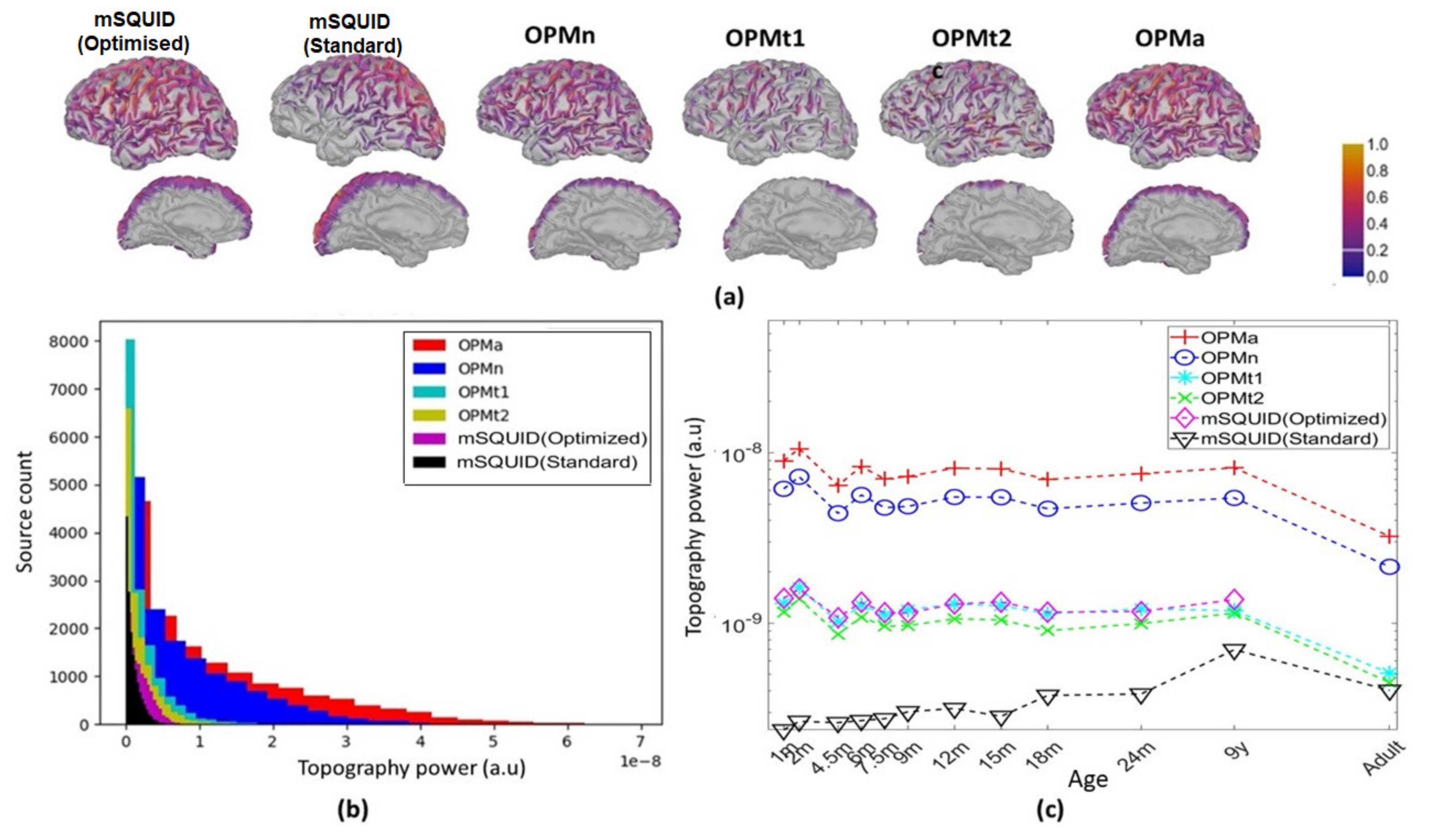
When considering the metrics for topography power, we found that the OPMa array performed significantly better than the SQUID array. This finding is in line with previous simulations of alkali OPMs [
14,
15]. Livanainen et al. [
15] reported that the average relative power (vs. an mSQUID) was 7.5 for nOPM and 5.3 for tOPM. Our results for a
4He OPM showed an 8.9-fold gain for aOPM (relative to an mSQUID) with the adult head model. Likewise, the OPMa outperformed the SQUID array with regard to total information capacity and sensitivity. Regarding OPMn alone, (the most technically similar to an mSQUID array), OPMn also brought benefits compared to SQUID, except for when it came to the total information. This result differs from what has been previously reported for alkali OPM, where both of the OPM arrays (nOPM and tOPM) provided more information than SQUID. This can be explained by the lower sensitivity of
4He OPM, set to 40 fT/
in this simulation study. However, combining all measurement axes, the aOPM array conveyed significantly more information than SQUID. As with the alkali OPM simulations, the tangential OPM (
t1 and
t2 OPM together) provided more information than nOPM did. This can be easily explained by the number of sensors (204 for tOPM vs. 102 for nOPM). However, if only one tangential axis is considered (
t1 or
t2 OPM, see
Figure 5), the total information was (as expected) lower than for nOPM. This also means that normal and tangential measurement axes carry independent information. Since the total information conveyed by aOPM was higher than nOPM and tOPM separately, these measurements are not redundant. This finding is in line with previous studies, in which biomagnetic source modeling was more accurate when a three-axis measurement of the brain or cardiac magnetic field was available [
35,
38,
39].
Our sensitivity map results also suggest that three-axis measurement provides a more exhaustive recording of the brain’s magnetic field. The results revealed that the OPMa array was more sensitive to tangentially oriented sources (
), relative to an mSQUID. These sources are poorly visualized by current MEG systems; this is mainly why EEG is usually combined with MEG to improve brain activity recordings. Ahlfors et al. [
32] performed a quantitative assessment of the contributions of radial vs. tangential sources to MEG and EEG, by using the sensitivity map metric originally developed by Huang et al. [
41]. A gain in sensitivity to radially oriented sources (
, preferentially recorded by mSQUID is also observed with OPMa, mainly for deep sources. This increased sensitivity of three axes OPM array to various sources orientations has never been reported in previous studies on alkali OPM [
14,
15]. This result suggests that the three-axis
4He OPM array simulated here can record brain sources more exhaustively. In principle, combined EEG recording should be less frequently required with this kind of OPM array. However, this hypothesis needs to be confirmed in a comparative study of real brain recordings by
4He OPMs combined (or not) with EEG.
In the present work, we assessed the respective contributions of volume and primary currents to the signals measured by OPM and SQUIDs. Our results are in line with those previous simulations of alkali OPMs [
15]. The PV values (for the signal measured by tangential axes of
4He OPM) close to one (1.02 for
t1 and
t2 OPM) indicated that the volume and primary currents make equivalent contributions. This can be viewed as an advantage as it suggests that tangential axes can measure signals usually recorded by EEG; the latter technique is more sensitive to volume currents, while MEG is more sensitive to primary currents). This finding is also in line with our sensitivity map results and confirms that the OPM’s tangential axes will probably provide better recordings of brain sources poorly visualized by current SQUID MEG and that require the combination of EEG and MEG [
32]. The volume current’s contribution to the tangential axis signal can also be viewed as a drawback as it will mask the primary current. However, our simulated TP values (0.28 for
t1 and
t2 OPM) suggest that the volume current did not totally cancel the primary current. Regarding OPMn, the magnetic field recorded along this axis is mainly related to the primary current’s contribution, since the PV value is much greater than one. However, the volume current still makes a contribution. The SQUID array (MEG) and the OPMn array had similar PV and TP values.
We also assessed the accuracy of brain source localization with a
4He OPM sensor array by calculating the PLE and SD metrics introduced by Hauk et al. [
42]. Our results showed that the PLE for brain source localization was lower for the OPMn array (2.4 mm) than for the mSQUID (2.8 mm). The gain in source localization accuracy was even greater for the OPMa array (2.3 mm). The SD of the brain source localized with OPMn array was also lower (3.5 mm) than that of the mSQUID (4.2 mm); again, this result was even better for the OPMa (3 mm). On the basis of these current simulations and the L2-norm minimum norm estimate used to compute the brain sources, the
4He OPM array was more accurate and yielded more focused brain source localizations. Livanainen et al. [
15] used the PSF to assess the advantage of an OPM array with regard to source localization accuracy. The researchers reported that the alkali OPM and SQUID arrays gave similar localization accuracies for minimum-norm estimation, however, they also reported that the OPM array gave a greater spatial resolution. Our results go beyond this statement. This disparity might be due to our use of different metrics (PLE and SD) for the PSF and the CTF.
4.3. Advantages of the 4He OPM with Infant, Child and Adult Subjects
Another salient result of the present study was the first quantitative assessment of the benefits of an OPM array for use with children and infants, relative to SQUID-based MEG recordings. We distinguished between two uses for all child and infant head models: mSQUID (optimized) corresponded to a MEG helmet of the right size for the subject’s size, with a scalp-sensor distance everywhere of two cm; mSQUID (standard) was more representative of real MEG assessments, in which the top of the head is placed close to the MEG helmet. This distinction is particularly important for children and infants, where the head is markedly smaller than the rigid SQUID MEG helmet and thus the scalp-sensor distance is greater. As mentioned in the Introduction, dedicated baby MEG systems are not widely available; here, mSQUID (optimized) corresponds to these devices. In normal MEG systems (as modelled by our mSQUID (standard) configuration), the top of the child’s or infant’s head is placed against the helmet; thus, the scalp-sensor distance is greater than two cm for the other parts of the head.
Considering the topography power, the total information capacity and the sensitivity metrics, OPMa still outperformed SQUID arrays for all subject ages. As expected, the benefit for the nine-year-old child (relative to the adult head model) was greater for OPMa vs. mSQUID (standard) then for OPMa vs. mSQUID (optimized). The benefit for topography power and sensitivity with the OPMa array vs. mSQUID (standard) was significantly greater for the (smaller) infant head than for the nine-year-old child model. Considering OPMn alone, it is also noteworthy that total information was increased relative to mSQUID standard array for infants, which was not observed for the adult head. These findings are the first quantitative indications of how the OPM array–scalp distance can affect the information content and the sensitivity of MEG recordings in children and infants. It emphasizes the particular value of OPM sensors for MEG recordings in children and infants due to placement on the scalp. A 4He OPM operates at room temperature (no heating occurs, in contrast to alkali OPMs) and does not have heat dissipation issues; hence, the device can be placed close to the scalp and so is particularly well suited to MEG recordings in infants and children.
With regard to TP and PV, the results for the OPM tangential axes were similar for adults, children, and infants. However, OPMn gave significantly higher PV values than either mSQUID (standard) or mSQUID (optimized)—showing that the primary current contributes more to MEG signals recorded with OPMn than those recorded with an mSQUID. This result suggests that the primary current contributes more to MEG signals, in view of the higher-amplitude signals typically recorded in children and infants [
43,
44]. The significant difference between OPMn and mSQUID might be due to the lower sensor-scalp distance, which optimizes the recording of the brain’s magnetic field, notably in infants. Regarding the TP parameter, the values for OPMn were close to one; hence, the volume currents (which are even greater in children and infants as the skull is less ossified) did not mask the greater primary current contribution to the MEG signals (as shown by higher PV values). As expected, these differences were even greater when considering mSQUID (standard) instead of mSQUID (optimized).
The OPMn array, and notably the OPMa array, gave smaller PLE and SD values, thus confirming that OPM arrays provide more accurate, focused brain source localization in children and infants. We observed a significant effect of age on difference between OPMa and mSQUID (optimized) or mSQUID (standard); the smaller the head size, the greater the gain in source location accuracy. Our values showed that the differences in PLE and SD between OPMa and mSQUID (standard) were, respectively, 0.17 mm and 0.9 mm for the nine-year-old child, while these differences were 0.18 mm and 1 mm for the one-month-old baby, corresponding to an increase in source localization accuracy of 9.15% and focality of 6.71%.
5. Conclusions and Perspectives
Overall, our results confirm the significant advantages of a three-axis 102-sensor
4He OPM array, relative to an mSQUID counterpart. We extended our simulations to children and infants of different ages and found that the added value achieved with an OPM array is even greater at smaller head sizes; indeed, the brain source–sensor distance becomes increasingly critical. These results were obtained by simulating a
4He OPM with a sensitivity of 40 fT/
. Despite the
4He OPM array’s low sensitivity, its three-axis measurement and its proximity to the scalp meant that it outperformed the mSQUID. Our results were also in line with previous simulations of alkali OPM sensors. Thanks to ongoing development, the
4He OPM’s low sensitivity is now rising; a value of 30 fT/
was reported recently [
22]. This increase in sensitivity might lead to a further improvement, relative to the results reported here.
The present simulation study compared a 102-sensor OPM array with the 102-sensor mSQUID array found in commercial MEG devices (MEGIN, Espoo, Finland) and previously published simulations of alkali OPM arrays. Our work should now be extended by simulating data with smaller three-axis 4He OPM arrays, in order to define the minimum number of OPMs required to achieve much the same performance levels as a standard mSQUID array. Furthermore, other MEG devices (such as those produced by CTF, San Diego, CA) feature a larger number of mSQUIDs. Lastly, it would be interesting to extend this work on the 4He OPM array to fetal brain data. However, modelling the womb and developing a fetal head model would be particularly challenging.


 ,
, 


