
Estimation of Organizational Competitiveness by a Hybrid of One-Dimensional Convolutional Neural Networks and Self-Organizing Maps Using Physiological Signals for Emotional Analysis of Employees

 ,
, 
 , and
, and
Abstract
:1. Introduction
2. Materials and Methods
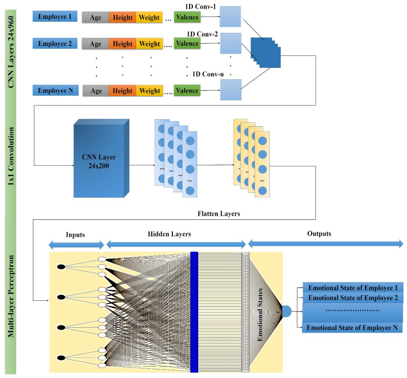
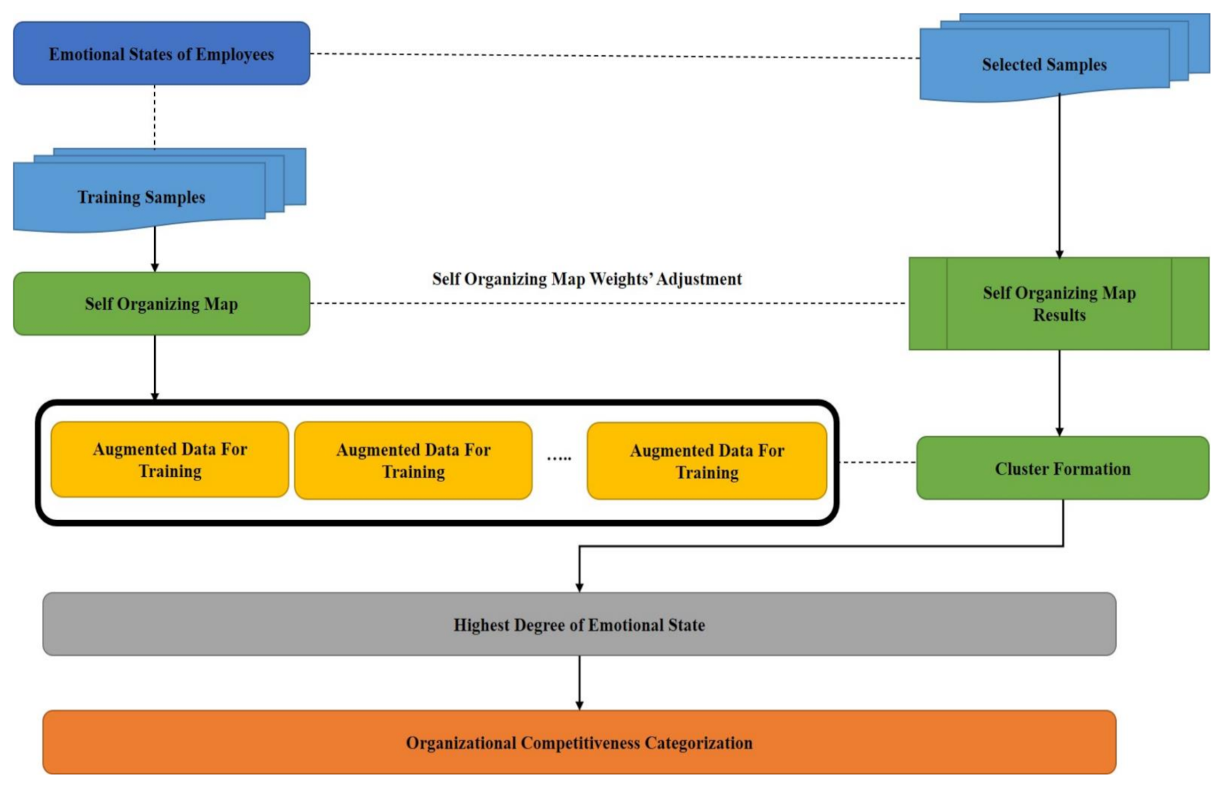
2.1. Dataset for the Proposed Work
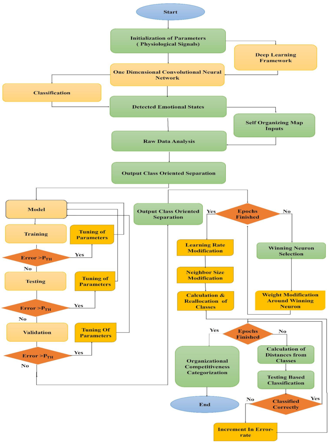
2.2. Emotion Classification through the Convolutional Neural Network
- Instead of matrix operations, basic array operations are required for forward and backward propagation in the ODCNN, which implies that the computational complexity of the ODCNN is less than that of the TDCNN.
- Recent investigations have indicated that the ODCNN with generally shallow designs (e.g., fewer neurons and hidden layers) can perform learning (for taxing operations), including 1D input data.
- Typically, a TDCNN demands additional deep models to deal with such cases. Networks with shallow structures are much simpler for training and execution.
- Usually, preparing deeper TDCNNs demands a particular setup for hardware. However, the feasibility of any processor execution over a standard computer, moderately quick for preparing the ODCNN with some neurons (e.g., fewer than 50) and hidden layers (e.g., two or fewer), is straightforward.
- Fewer computational necessities make the ODCNN appropriate for low-cost, real-time, and well-suited applications, particularly on portable or hand-held gadgets.
- Hidden layers of the MLP and hidden layers of the CNN are used.
- In every layer of the CNN, the kernel/filter size is selected.
- In each CNN layer, a subsampling factor is selected.
- The activation and pooling functions are selected.
Backward and Forward Propagation in the One-Dimensional Convolutional Neural Network
| Algorithm 1. Backward and forward propagation in the one-dimensional convolutional neural network (ODCNN) |
 |
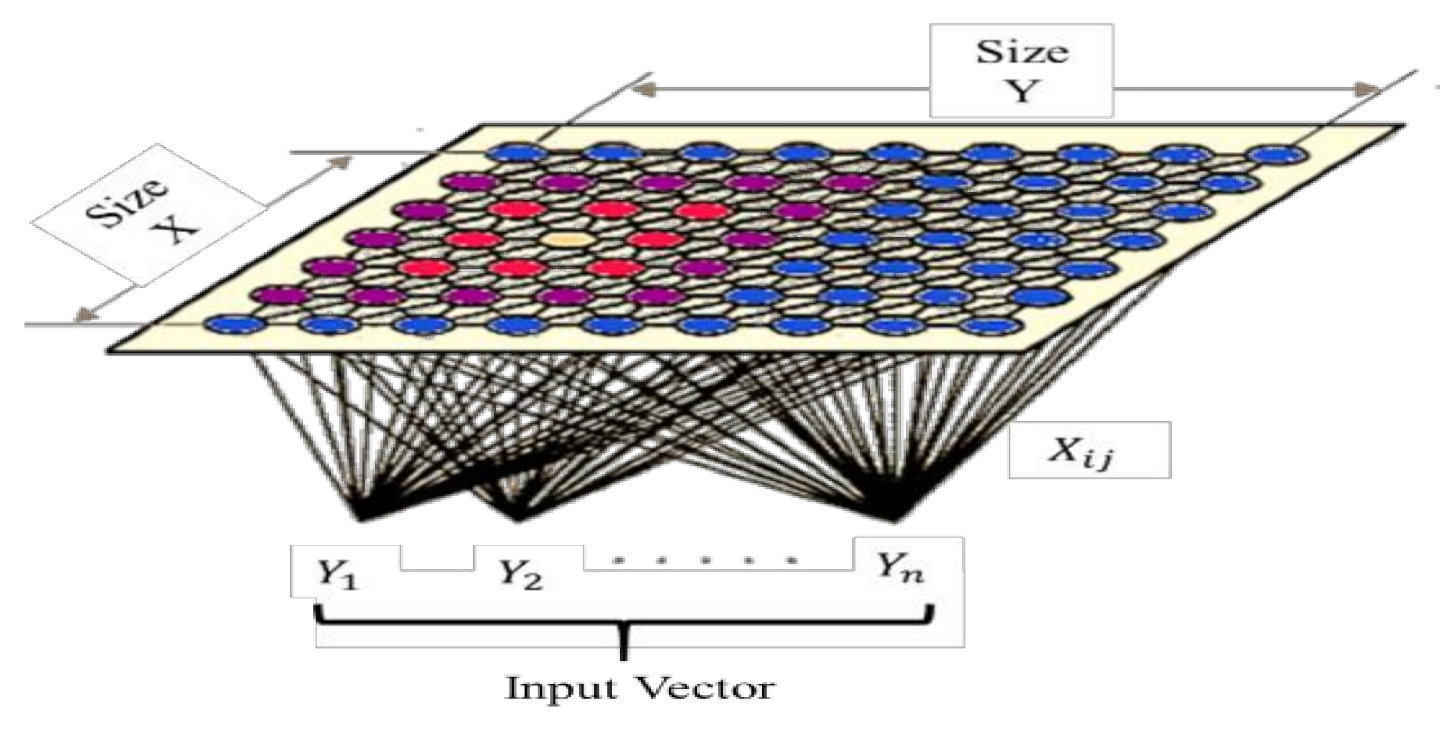
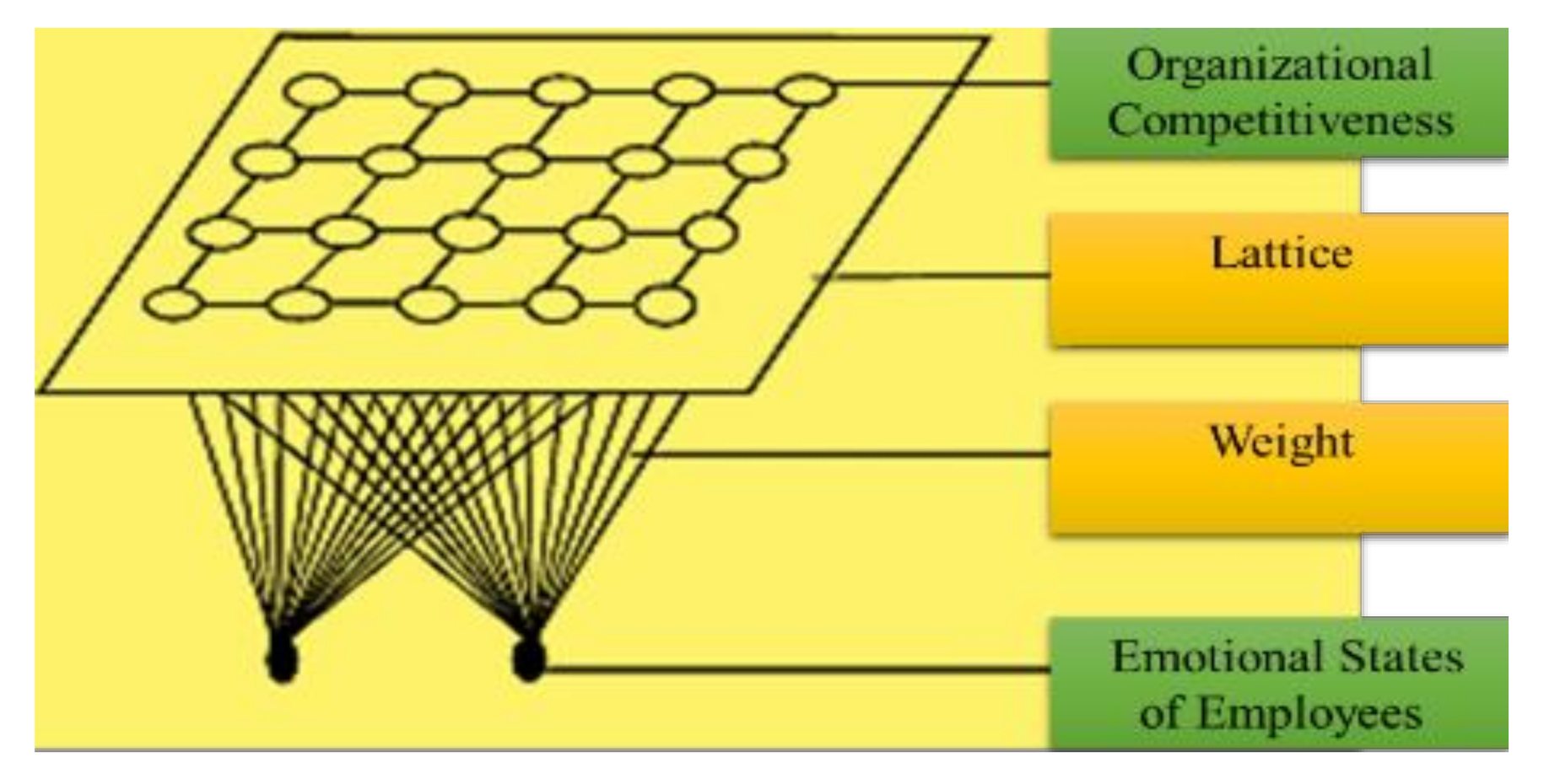
2.3. Detection of Organizational Competitiveness Based on the Self-Organizing Map
- The U represents the current iteration.
- The total number of iterations of the network is represented by o, the limit of iterations.
- For the decay of the learning rate and radius, the time constraint is represented by λ.
- The row coordinate of the node matrix is represented by j.
- The column coordinate of the node matrix is represented by k.
- The distance between the BMU and node is represented by e.
- The weight vector is represented by x.
- The connection weight between the input vector occurrence and ith and jth nodes in the matrix (for the tth iteration) is represented by x_ij(t).
- The input vector is represented by y.
- The instance of the input vector at the tth iteration is represented by y(t).
- The learning rate is represented by β(t), in the [0,1] range. To guarantee the coverage of the network, it diminishes with time.
- The neighborhood operation is represented by _ij(t), which diminishes and addresses the distance between the BMU and the i and j nodes and its effect on the learning rate at the tth iteration.
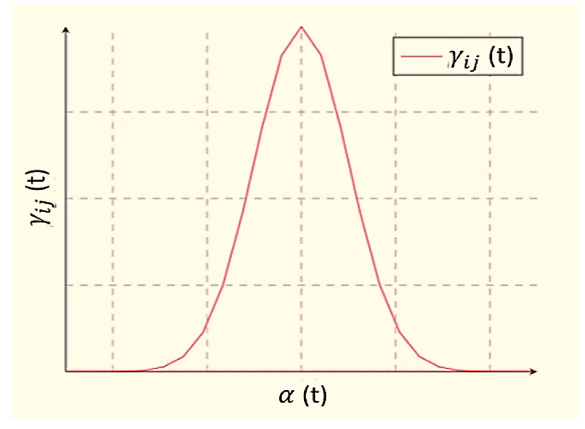
- The neighborhood operations radius is represented by (t), which determines (in the 2D matrix) how far neighbor nodes are inspected with the update of the vectors. It is progressively diminished after some time. Figure 5 presents the SOM with the input and output identification.
Update of Parameters in the Self-Organizing Map
| Algorithm 2. Categorization of organizational competitiveness based on the self-organizing map |
 |
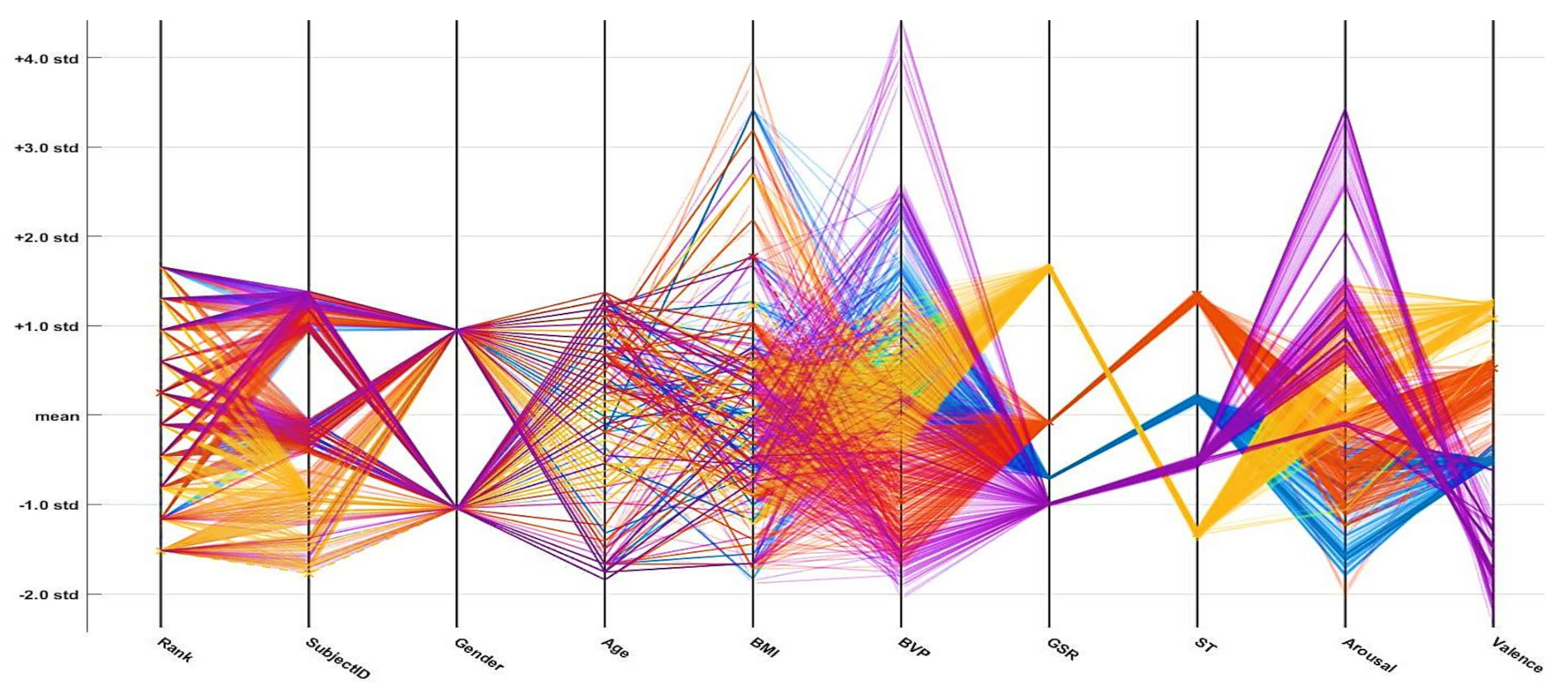
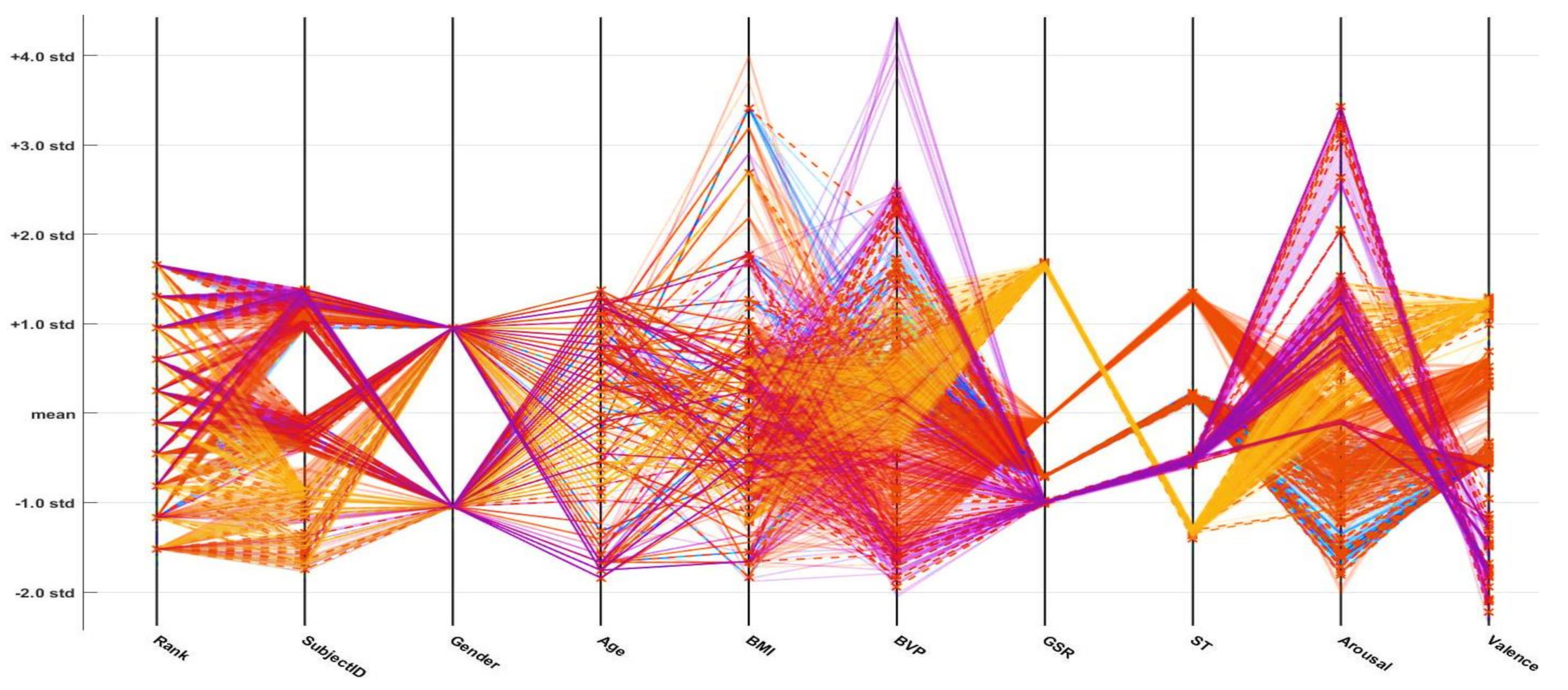
3. Experimental Results
3.1. Emotional State Detection
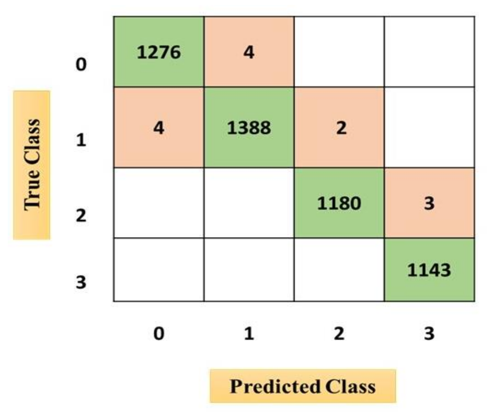
3.1.1. One-Dimensional Convolutional Neural Network
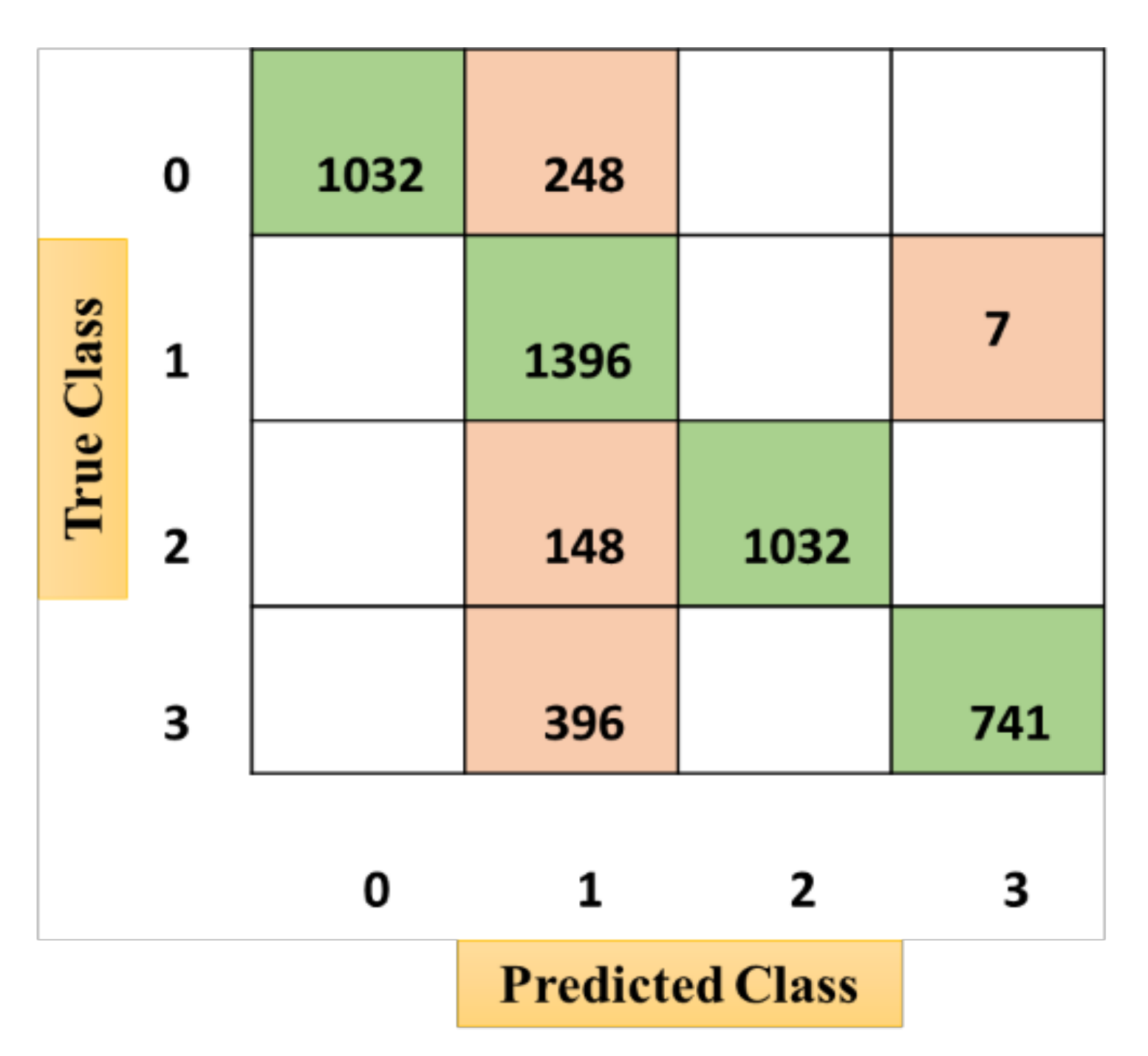
3.1.2. Support Vector Machine
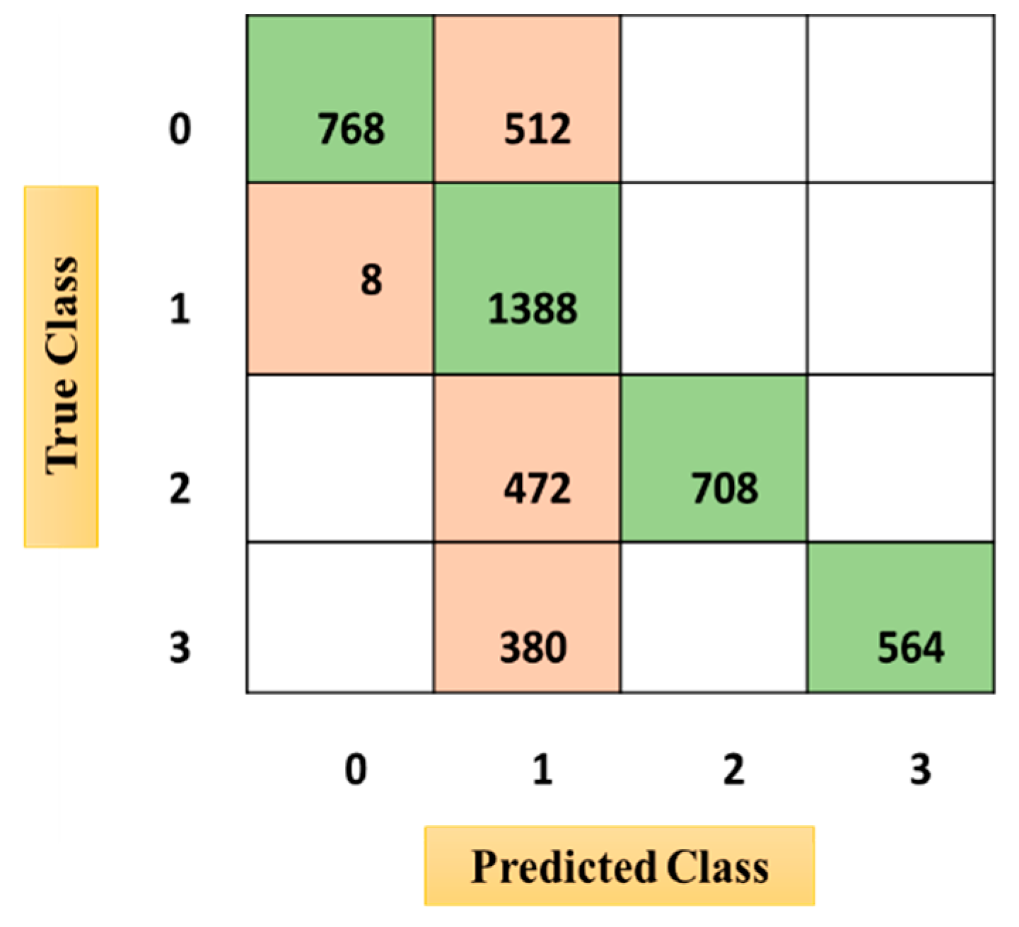
3.1.3. Ensemble RUSBoosted Tree (ERT)
3.2. One-Dimensional Convolutional Neural Network Structure Optimization
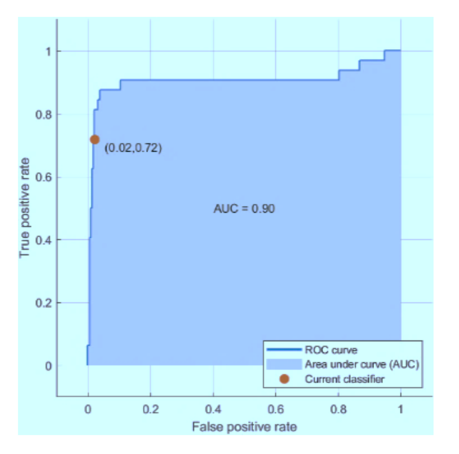
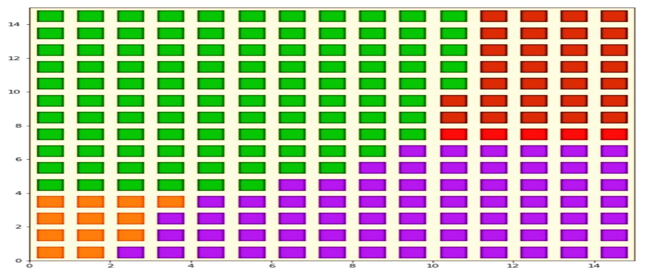
3.3. Organizational Competitiveness Categorization through the Self-Organizing Map
4. Discussion
5. Conclusions and Future Work
Author Contributions
Funding
Institutional Review Board Statement
Informed Consent Statement
Data Availability Statement
Acknowledgments
Conflicts of Interest
References
- Porteous, J.D. Home: The territorial core. Geogr. Rev. 1976, 66, 383. [Google Scholar] [CrossRef]
- Zheng, W.-L.; Zhu, J.-Y.; Lu, B.-L. Identifying stable patterns over time for emotion recognition from EEG. IEEE Trans. Affect. Comput. 2019, 10, 417–429. [Google Scholar] [CrossRef] [Green Version]
- Kowalczuk, Z.; Czubenko, M.; Merta, T. Interpretation and modeling of emotions in the management of autonomous robots using a control paradigm based on a scheduling variable. Eng. Appl. Artif. Intell. 2020, 91, 103562. [Google Scholar] [CrossRef]
- Hossain, M.S.; Muhammad, G. Emotion recognition using deep learning approach from audio–visual emotional big data. Inf. Fusion 2019, 49, 69–78. [Google Scholar] [CrossRef]
- Li, Z.; Qiu, L.; Li, R.; He, Z.; Xiao, J.; Liang, Y.; Wang, F.; Pan, J. Enhancing BCI-based emotion recognition using an improved particle Swarm optimization for feature selection. Sensors 2020, 20, 3028. [Google Scholar] [CrossRef]
- Kowalczuk, Z.; Czubenko, M. Computational approaches to modeling artificial emotion—An overview of the proposed solutions. Front. Robot. AI 2016, 3, 21. [Google Scholar] [CrossRef] [Green Version]
- Wioleta, S. Using physiological signals for emotion recognition. In Proceedings of the 6th International Conference on Human System Interactions (HSI), Gdańsk, Poland, 6–8 June 2013; pp. 556–561. [Google Scholar]
- Udovičić, G.; Ðerek, J.; Russo, M.; Sikora, M. Wearable emotion recognition system based on GSR and PPG signals. In Proceedings of the 2nd International Workshop on Multimedia for Personal Health and Health Care (ACM), Mountain View, CA, USA, 23–27 October 2017; pp. 53–59. [Google Scholar]
- El Ayadi, M.; Kamel, M.; Karray, F. Survey on speech emotion recognition: Features, classification schemes, and databases. Pattern Recognit. 2011, 44, 572–587. [Google Scholar] [CrossRef]
- Lin, Y.-P.; Wang, C.-H.; Jung, T.-P.; Wu, T.-L.; Jeng, S.-K.; Duann, J.-R.; Chen, J.-H. EEG-based emotion recognition in music listening. IEEE Trans. Biomed. Eng. 2010, 57, 1798–1806. [Google Scholar] [CrossRef]
- Harms, M.B.; Martin, A.; Wallace, G.L. Facial emotion recognition in Autism spectrum disorders: A review of behavioral and neuroimaging studies. Neuropsychol. Rev. 2010, 20, 290–322. [Google Scholar] [CrossRef]
- Ali, M.; Mosa, A.H.; Al Machot, F.; Kyamakya, K. emotion recognition involving physiological and speech signals: A comprehensive review. In Recent Advances in Nonlinear Dynamics and Synchronization; Springer: Cham, Switzerland, 2018; pp. 287–302. [Google Scholar]
- Makikawa, M.; Shiozawa, N.; Okada, S. Fundamentals of wearable sensors for the monitoring of physical and physiological changes in daily life. In Wearable Sensors; Academic Press: Cambridge, MA, USA, 2014; pp. 517–541. [Google Scholar]
- Yoo, G.; Seo, S.; Hong, S.; Kim, H. Emotion extraction based on multi bio-signal using back-propagation neural network. Multimed. Tools Appl. 2018, 77, 4925–4937. [Google Scholar] [CrossRef]
- Li, C.; Xu, C.; Feng, Z. Analysis of physiological for emotion recognition with the IRS model. Neurocomputing 2016, 178, 103–111. [Google Scholar] [CrossRef]
- Ayata, D.; Yaslan, Y.; Kamaşak, M. Emotion recognition via galvanic skin response: Comparison of machine learning algorithms and feature extraction methods. Istanb. Univ. J. Electr. Electron. Eng. 2017, 17, 3147–3156. [Google Scholar]
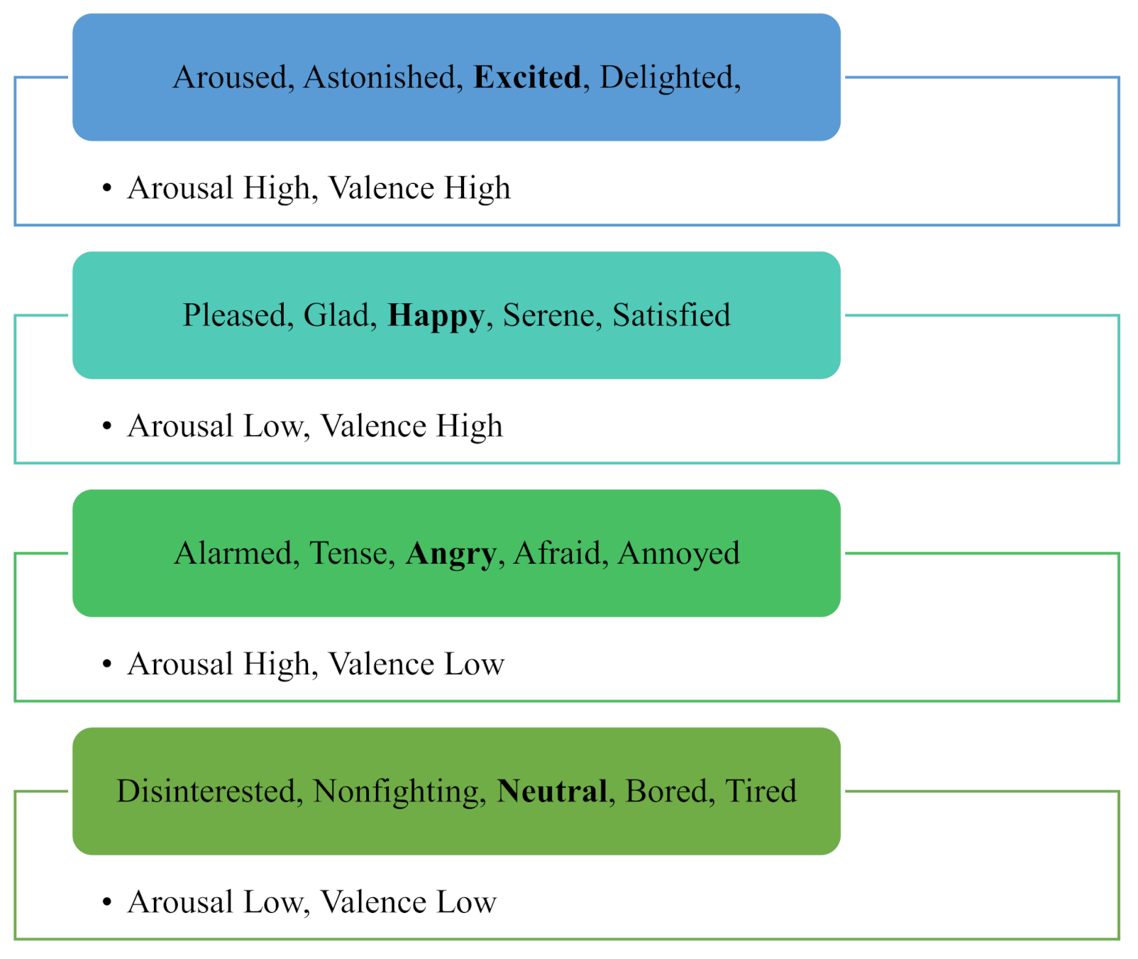
- Yik, M.; Russell, J.A.; Steiger, J.H. A 12-point circumplex structure of core affect. Emotion 2011, 11, 705–731. [Google Scholar] [CrossRef] [Green Version]
- Posner, J.; Russell, J.A.; Peterson, B.S. The circumplex model of affect: An integrative approach to affective neuroscience, cognitive development, and psychopathology. Dev. Psychopathol. 2005, 17, 715–734. [Google Scholar] [CrossRef]
- Dzedzickis, A.; Kaklauskas, A.; Bucinskas, V. Human emotion recognition: Review of sensors and methods. Sensors 2020, 20, 592. [Google Scholar] [CrossRef] [Green Version]
- Bergstrom, J.R.; Duda, S.; Hawkins, D.; McGill, M. Physiological response measurements. In Eye Tracking in User Experience Design; Elsevier: Amsterdam, The Netherlands, 2014; pp. 81–108. [Google Scholar]
- Seo, J.; Laine, T.H.; Sohn, K.-A. An exploration of machine learning methods for robust boredom classification using EEG and GSR data. Sensors 2019, 19, 4561. [Google Scholar] [CrossRef] [Green Version]
- Greco, A.; Valenza, G.; Citi, L.; Scilingo, E.P. Arousal and valence recognition of affective sounds based on electrodermal activity. IEEE Sens. J. 2017, 17, 716–725. [Google Scholar] [CrossRef]
- LeCun, Y.; Bengio, Y.; Hinton, G. Deep learning. Nature 2015, 521, 436–444. [Google Scholar] [CrossRef]
- Zhang, W.; Zhang, Y.; Zhai, J.; Zhao, D.; Xu, L.; Zhou, J.; Li, Z.; Yang, S. Multi-source data fusion using deep learning for smart refrigerators. Comput. Ind. 2018, 95, 15–21. [Google Scholar] [CrossRef]
- Aslam, B.; Alrowaili, Z.A.; Khaliq, B.; Manzoor, J.; Raqeeb, S.; Ahmad, F. Ozone depletion identification in stratosphere through faster region-based convolutional neural network. Comput. Mater. Contin. 2021, 68, 2159–2178. [Google Scholar] [CrossRef]
- Cropanzano, R.; Prehar, C.A.; Chen, P.Y. Using social exchange theory to distinguish procedural from interactional justice. Group Organ. Manag. 2002, 27, 324–351. [Google Scholar] [CrossRef]
- Luthans, F.; Norman, S.M.; Avolio, B.J.; Avey, J.B. The mediating role of psychological capital in the supportive organizational climate—Employee performance relationship. J. Organ. Behav. 2008, 29, 219–238. [Google Scholar] [CrossRef] [Green Version]
- Anwar, M.S.; Aslam, M.; Tariq, M.R. Temporary job and its impact on employee performance. Glob. J. Manag. Bus. Res. 2011, 11, 8. [Google Scholar]
- Basu, S.; Fernald, J.G.; Shapiro, M.D. Productivity growth in the 1990s: Technology, utilization, or adjustment? Carnegie-Rochester Conf. Ser. Public Policy 2001, 55, 117–165. [Google Scholar] [CrossRef] [Green Version]
- Kadoya, Y.; Khan, M.S.R.; Watanapongvanich, S.; Binnagan, P. emotional status and productivity: Evidence from the special economic zone in Laos. Sustainability 2020, 12, 1544. [Google Scholar] [CrossRef] [Green Version]
- Relich, M. The impact of ICT on labor productivity in the EU. Inf. Technol. Dev. 2017, 23, 706–722. [Google Scholar] [CrossRef]
- Belorgey, N.; Lecat, R.; Maury, T.-P. Determinants of productivity per employee: An empirical estimation using panel data. Econ. Lett. 2006, 91, 153–157. [Google Scholar] [CrossRef] [Green Version]
- Boles, M.; Pelletier, B.; Lynch, W. The relationship between health risks and work productivity. J. Occup. Environ. Med. 2004, 46, 737–745. [Google Scholar] [CrossRef]
- Bubonya, M.; Cobb-Clark, D.A.; Wooden, M. Mental health and productivity at work: Does what you do matter? Labour Econ. 2017, 46, 150–165. [Google Scholar] [CrossRef] [Green Version]
- Saarni, C. The Development of Emotional Competence; Guilford Press: New York, NY, USA, 1999. [Google Scholar]
- DiMaria, C.H.; Peroni, C.; Sarracino, F. Happiness matters: Productivity gains from subjective well-being. J. Happiness Stud. 2019, 21, 139–160. [Google Scholar] [CrossRef]
- Kim, J.; Fesenmaier, D.R. Measuring emotions in real time: Implications for tourism experience design. J. Travel Res. 2015, 54, 419–429. [Google Scholar] [CrossRef]
- Liang, Y.; Chen, Z.; Liu, G.; Elgendi, M. A new, short-recorded photoplethysmogram dataset for blood pressure monitoring in China. Sci. Data 2018, 5, 1–7. [Google Scholar] [CrossRef] [Green Version]
- Liang, Y.; Liu, G.; Chen, Z.; Elgendi, M. PPG-BP Database. Figshare. Dataset. 2018. Available online: https://figshare.com/articles/dataset/PPG-BP_Database_zip/5459299/3 (accessed on 25 May 2021).
- Vettigli, G. MiniSom: Minimalistic and NumPy-Based Implementation of the Self Organizing Map. 2018. Available online: https://github.com/JustGlowing/minisom/ (accessed on 25 May 2021).
- Sharma, K.; Wagner, M.; Castellini, C.; van den Broek, E.L.; Stulp, F.; Schwenker, F. A Functional Data Analysis Approach for Continuous 2-D Emotion Annotations; IOS Press: Amsterdam, The Netherlands, 2019; pp. 41–52. [Google Scholar]
- Abdel-Hamid, O.; Mohamed, A.-R.; Jiang, H.; Penn, G. Applying convolutional neural networks concepts to hybrid NN-HMM model for speech recognition. In Proceedings of the IEEE International Conference on Acoustics, Speech and Signal Processing (ICASSP), Kyoto, Japan, 25–30 March 2012; pp. 4277–4280. [Google Scholar]
- Zhang, Y.; Wallace, B. A sensitivity analysis of (and practitioners’ guide to) convolutional neural networks for sentence classification. arXiv 2015, arXiv:1510.03820. [Google Scholar]
- Ding, X.; He, Q. Energy-fluctuated multiscale feature learning with deep ConvNet for intelligent spindle bearing fault diagnosis. IEEE Trans. Instrum. Meas. 2017, 66, 1926–1935. [Google Scholar] [CrossRef]
- Kiranyaz, S.; Ince, T.; Gabbouj, M. Real-time patient-specific ECG classification by 1-D convolutional neural networks. IEEE Trans. Biomed. Eng. 2015, 63, 664–675. [Google Scholar] [CrossRef]
- Kiranyaz, S.; Ince, T.; Hamila, R.; Gabbouj, M. Convolutional neural networks for patient-specific ECG classification. In Proceedings of the 37th Annual International Conference of the IEEE Engineering in Medicine and Biology Society (EMBC), Milano, Italy, 25–29 August 2015; Volume 2015, pp. 2608–2611. [Google Scholar]
- Kiranyaz, S.; Ince, T.; Gabbouj, M. Personalized monitoring and advance warning system for cardiac arrhythmias. Sci. Rep. 2017, 7, 1–8. [Google Scholar] [CrossRef]
- Avci, O.; Abdeljaber, O.; Kiranyaz, S.; Hussein, M.; Inman, D.J. Wireless and real-time structural damage detection: A novel decentralized method for wireless sensor networks. J. Sound Vib. 2018, 424, 158–172. [Google Scholar] [CrossRef]
- Avci, O.; Abdeljaber, O.; Kiranyaz, S.; Inman, D. Structural damage detection in real time: Implementation of 1D convolutional neural networks for SHM applications. In Structural Health Monitoring & Damage Detection; Springer: Cham, Switzerland, 2017; Volume 7, pp. 49–54. [Google Scholar]
- Abdeljaber, O.; Avci, O.; Kiranyaz, S.; Gabbouj, M.; Inman, D.J. Real-time vibration-based structural damage detection using one-dimensional convolutional neural networks. J. Sound Vib. 2017, 388, 154–170. [Google Scholar] [CrossRef]
- Avci, O.; Abdeljaber, O.; Kiranyaz, S.; Boashash, B.; Sodano, H.; Inman, D.J. Efficiency validation of one dimensional convolutional neural networks for structural damage detection using a SHM benchmark data. In Proceedings of the 25th International Congress on Sound and Vibration (ICSV 25), Hiroshima, Japan, 8–12 July 2018; pp. 4600–4607. [Google Scholar]
- Abdeljaber, O.; Avci, O.; Kiranyaz, M.S.; Boashash, B.; Sodano, H.; Inman, D.J. 1-D CNNs for structural damage detection: Verification on a structural health monitoring benchmark data. Neurocomputing 2018, 275, 1308–1317. [Google Scholar] [CrossRef]
- Acharya, U.R.; Fujita, H.; Oh, S.L.; Hagiwara, Y.; Tan, J.H.; Adam, M. Application of deep convolutional neural network for automated detection of myocardial infarction using ECG signals. Inf. Sci. 2017, 415–416, 190–198. [Google Scholar] [CrossRef]
- Xiong, Z.; Stiles, M.; Zhao, J. Robust ECG signal classification for the detection of atrial fibrillation using novel neural networks. In Proceedings of the Computing in Cardiology Conference (CinC), Rennes, France, 24–27 September 2017; pp. 1–4. [Google Scholar]
- Acharya, U.R.; Oh, S.L.; Hagiwara, Y.; Tan, J.H.; Adam, M.; Gertych, A.; Tan, R.S. A deep convolutional neural network model to classify heartbeats. Comput. Biol. Med. 2017, 89, 389–396. [Google Scholar] [CrossRef] [PubMed]
- Awrejcewicz, J.; Krysko, A.; Pavlov, S.; Zhigalov, M.; Krysko, V. Chaotic dynamics of size dependent Timoshenko beams with functionally graded properties along their thickness. Mech. Syst. Signal Process. 2017, 93, 415–430. [Google Scholar] [CrossRef]
- Zheng, Q.; Yang, M.; Yang, J.; Zhang, Q.; Zhang, X. Improvement of generalization ability of deep CNN via implicit regularization in two-stage training process. IEEE Access 2018, 6, 15844–15869. [Google Scholar] [CrossRef]
- Zheng, Q.; Tian, X.; Yang, M.; Wu, Y.; Su, H. PAC-Bayesian framework based drop-path method for 2D discriminative convolutional network pruning. Multidimens. Syst. Signal Process. 2019, 31, 793–827. [Google Scholar] [CrossRef]
- Alanazi, S.A. Toward identifying features for automatic gender detection: A corpus creation and analysis. IEEE Access 2019, 7, 111931–111943. [Google Scholar] [CrossRef]
- Graterol, W.; Diaz-Amado, J.; Cardinale, Y.; Dongo, I.; Lopes-Silva, E.; Santos-Libarino, C. Emotion detection for social robots based on NLP transformers and an emotion ontology. Sensors 2021, 21, 1322. [Google Scholar] [CrossRef]
- Kim, Y.; Choi, A. EEG-Based emotion classification using long short-term memory network with attention mechanism. Sensors 2020, 20, 6727. [Google Scholar] [CrossRef]
- Ince, T.; Kiranyaz, S.; Eren, L.; Askar, M.; Gabbouj, M. Real-time motor fault detection by 1-D convolutional neural networks. IEEE Trans. Ind. Electron. 2016, 63, 7067–7075. [Google Scholar] [CrossRef]
- Kiranyaz, S.; Avci, O.; Abdeljaber, O.; Ince, T.; Gabbouj, M.; Inman, D.J. 1-D convolutional neural networks and applications: A survey. Mech. Syst. Signal Process. 2021, 151, 107398. [Google Scholar] [CrossRef]


| Age (Years) | Mean ± Standard Deviation | 44.20 ± 11.50 |
|---|---|---|
| Gender | Female | 574 (47.8%) |
| Male | 626 (52.2%) | |
| Organizational Ranking | Rank 1 | 130 (10.8%) |
| Rank 2 | 131 (10.9%) | |
| Rank 3 | 121 (10.1%) | |
| Rank 4 | 127 (10.6%) | |
| Rank 5 | 123 (10.3%) | |
| Rank 6 | 135 (11.3%) | |
| Rank 7 | 100 (8.3%) | |
| Rank 8 | 125 (10.4%) | |
| Rank 9 | 110 (9.2%) | |
| Rank 10 | 98 (8.2%) |
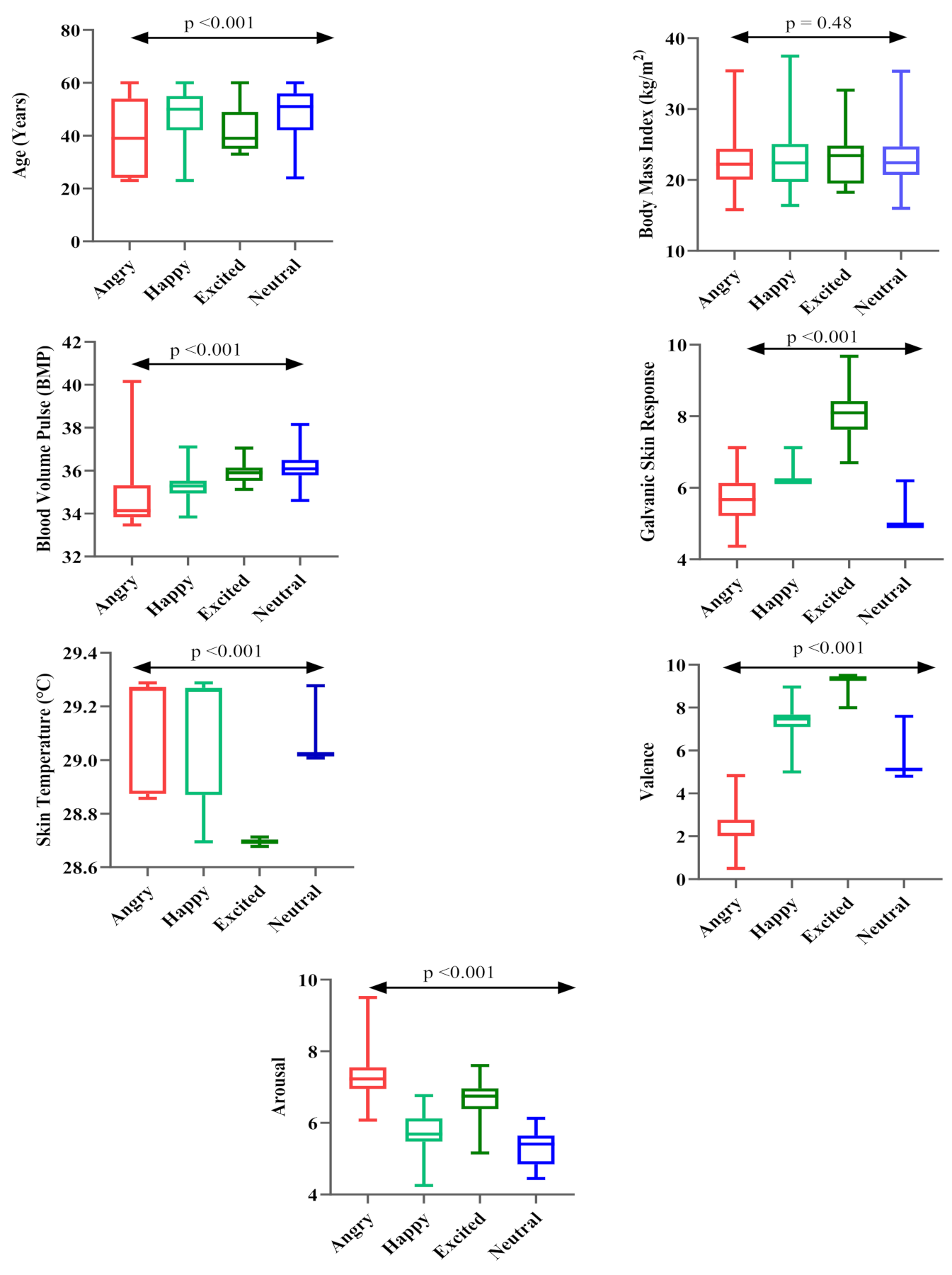
| Emotional Status (n, %) | Age | Body Mass Index | Blood Volume Pulse | Galvanic Skin Response | Skin Temperature | Valence | Arousal |
|---|---|---|---|---|---|---|---|
| Angry (236, 19.7%) | 39.72 ± 14.38 | 22.50 ± 3.50 | 34.81 ± 1.43 | 5.67 ± 0.67 | 29.14 ± 0.18 | 2.45 ± 0.82 | 7.41 ± 0.85 |
| Happy (349, 29.1%) | 46.26 ± 11.50 | 22.94 ± 4.27 | 35.30 ± 0.69 | 6.19 ± 0.05 | 29.08 ± 0.20 | 7.28 ± 0.60 | 5.74 ± 0.41 |
| Excited (295, 24.6%) | 41.88 ± 7.84 | 22.64 ± 3.14 | 35.88 ± 0.42 | 8.15 ± 0.70 | 28.69 ± 0.01 | 9.28 ± 0.23 | 6.71 ± 0.45 |
| Neutral (320, 26.7%) | 47.40 ± 10.47 | 22.75 ± 3.68 | 36.19 ± 0.61 | 4.95 ± 0.07 | 29.02 ± 0.01 | 5.38 ± 0.72 | 5.29 ± 0.44 |
| p-value | <0.001 | 0.48 | 0.001 | <0.001 | 0.001 | <0.001 | <0.001 |
| Correlation Analysis in the Angry Status | |||||||
|---|---|---|---|---|---|---|---|
| Age | Arousal | Valence | Skin Temperature | Galvanic Skin Response | Blood Volume Pulse | ||
| Body Mass Index | PC | 0.49 | −0.09 | 0.09 | 0.12 | 0.03 | −0.12 |
| p-value | <0.001 * | 0.15 | 0.16 | 0.07 | 0.64 | 0.06 | |
| Blood Volume Pulse | PC | −0.08 | 0.08 | −0.14 | −0.23 | 0.07 | |
| p-value | 0.20 | 0.20 | 0.01 * | <0.001 | 0.30 | ||
| Galvanic Skin Response | PC | −0.05 | −0.05 | −0.06 | 0.34 | ||
| p-value | 0.43 | 0.41 | 0.25 | 0.01 * | |||
| Skin Temperature | PC | 0.13 | −0.49 | 0.10 | |||
| p-value | 0.05 | <0.001 * | 0.09 | ||||
| Valence | PC | 0.14 | −0.53 | ||||
| p-value | 0.02 * | <0.001 * | |||||
| Arousal | PC | −0.09 | |||||
| p-value | 0.15 | ||||||
| Correlation Analysis in the Happy Status | |||||||
| Age | Arousal | Valence | Skin Temperature | Galvanic Skin Response | Blood Volume | ||
| Body Mass Index | PC | 0.28 | 0.04 | −0.04 | −0.06 | 0.06 | 0.01 |
| p-value | <0.001 * | 0.44 | 0.36 | 0.77 | 0.25 | 0.83 | |
| Blood Volume Pulse | PC | 0.06 | −0.17 * | 0.16 | 0.03 | 0.03 | |
| p-value | 0.26 | 0.001 * | 0.07 | 0.54 | 0.61 | ||
| Galvanic Skin Response | PC | 0.01 | 0.09 | 0.16 | −0.19 | ||
| p-value | 0.99 | 0.11 | 0.09 | 0.07 | |||
| Skin Temperature | PC | 0.03 | −0.08 | −0.42 * | |||
| p-value | 0.96 | 0.10 | 0.006 | ||||
| Valence | PC | −0.06 | 0.62 * | ||||
| p-value | 0.20 | <0.001 * | |||||
| Arousal | PC | −0.04 | |||||
| p-value | 0.45 | ||||||
| Correlation Analysis in the Excited Status | |||||||
| Age | Arousal | Valence | Skin Temperature | Galvanic Skin Response | Blood Volume Pulse | ||
| Body Mass Index | PC | 0.19 | 0.13 | 0.05 | 0.06 | 0.02 | −0.08 |
| p-value | <0.001 * | 0.09 | 0.34 | 0.28 | 0.71 | 0.15 | |
| Blood Volume Pulse | PC | 0.01 | −0.30 | −0.10 | 0.18 * | 0.02 | |
| p-value | 0.88 | 0.61 | 0.08 | 0.01 * | 0.99 | ||
| Galvanic Skin Response | PC | −0.04 | 0.08 | 0.06 | 0.01 | ||
| p-value | 0.44 | 0.13 | 0.28 | 0.86 | |||
| Skin Temperature | PC | −0.03 | −0.36 | −0.03 | |||
| p-value | 0.50 | 0.54 | 0.51 | ||||
| Valence | PC | 0.01 | 0.35 | ||||
| p-value | 0.82 | <0.001 * | |||||
| Arousal | PC | 0.15 | |||||
| p-value | 0.01 * | ||||||
| Correlation Analysis in the Neutral Status | |||||||
| Age | Arousal | Valence | Skin Temperature | Galvanic Skin Response | Blood Volume Pulse | ||
| Body Mass Index | PC | 0.24 | 0.01 | −0.13 | 0.09 | 0.10 | −0.08 |
| p-value | <0.01 * | 0.74 | 0.18 | 0.10 | 0.06 | 0.14 | |
| Blood Volume Pulse | PC | −0.14 | −0.005 | −0.006 | −0.14 | −0.14 | |
| p-value | 0.01 * | 0.933 | 0.91 | 0.08 | 0.01 * | ||
| Galvanic Skin Response | PC | 0.04 | 0.09 | 0.16 | 0.94 | ||
| p-value | 0.43 | 0.08 | 0.003 * | <0.001 * | |||
| Skin Temperature | PC | 0.04 | 0.11 | 0.19 | |||
| p-value | 0.41 | 0.04* | 0.001 * | ||||
| Valence | PC | −0.11 | 0.02 | ||||
| p-value | 0.03 * | 0.72 | |||||
| Arousal | PC | −0.01 | |||||
| p-value | 0.89 | ||||||
| Parameter | Value |
|---|---|
| Accuracy Rate | 99.8% |
| Total Misclassification Cost | 12 |
| Prediction Speed | ~420 obs/s |
| Training Time | 13.8652 s |
| Model Type | ODCNN |
| Parameter | Value |
|---|---|
| Accuracy | 83.5% |
| Total Misclassification Cost | 802 |
| Prediction Speed | ~1201 obs/s |
| Training Time | 11.8658 s |
| Model Type | Gaussian SVM |
| Kernel Function | Gaussian Kernel |
| Kernel Scale | 2.5 |
| Multiclass Method | One to Many |
| Parameter | Value |
|---|---|
| Accuracy | 71.4% |
| Total Misclassification Cost | 1398 |
| Prediction Speed | ~881 obs/s |
| Training Time | 14.5868 s |
| Model Type | Boosted Trees |
| Ensemble Method | RUSBoosted |
| Learner Type | Decision Tree |
| Maximum Number of Splits | 30 |
| Number of Learners | 20 |
| Configuration Number | Network Depth | Kernal Size | Learning Rate | Activation Function | Model Type | Accuracy (%) | Prediction Speed (obs/s) | Training Time (s) |
|---|---|---|---|---|---|---|---|---|
| 1 | 3 | 3 | 0.00005 | ELU | ODCNN | 95.53 | ~180 | 3.8862 |
| 2 | 3 | 5 | 0.00001 | ELU | ODCNN | 97.74 | ~204 | 4.2252 |
| 3 | 3 | 7 | 0.0005 | ELU | ODCNN | 92.92 | ~230 | 4.3711 |
| 4 | 3 | 9 | 0.0001 | ELU | ODCNN | 90.03 | ~308 | 6.1201 |
| 5 | 4 | 3 | 0.00005 | ELU | ODCNN | 91.47 | ~198 | 6.0529 |
| 6 | 4 | 5 | 0.00001 | ELU | ODCNN | 97.13 | ~276 | 9.8658 |
| 7 | 4 | 7 | 0.0005 | ELU | ODCNN | 96.22 | ~332 | 11.2355 |
| 8 | 4 | 9 | 0.0001 | ELU | ODCNN | 97.93 | ~412 | 13.1341 |
| 9 | 5 | 3 | 0.00005 | ELU | ODCNN | 98.79 | ~208 | 8.3424 |
| 10 | 5 | 5 | 0.00001 | ELU | ODCNN | 99.56 | ~302 | 11.0012 |
| 11 | 5 | 7 | 0.0005 | ELU | ODCNN | 99.80 | ~420 | 13.8652 |
| 12 | 5 | 9 | 0.0001 | ELU | ODCNN | 96.53 | ~538 | 15.4654 |
| 13 | 6 | 3 | 0.00005 | ELU | ODCNN | 93.76 | ~272 | 10.2232 |
| 14 | 6 | 5 | 0.00001 | ELU | ODCNN | 92.23 | ~399 | 12.1113 |
| 15 | 6 | 7 | 0.0005 | ELU | ODCNN | 95.02 | ~454 | 20.7345 |
| 16 | 6 | 9 | 0.0001 | ELU | ODCNN | 91.88 | ~688 | 22.8952 |
Publisher’s Note: MDPI stays neutral with regard to jurisdictional claims in published maps and institutional affiliations. |
© 2021 by the authors. Licensee MDPI, Basel, Switzerland. This article is an open access article distributed under the terms and conditions of the Creative Commons Attribution (CC BY) license (https://creativecommons.org/licenses/by/4.0/).
Share and Cite
Alanazi, S.A.; Alruwaili, M.; Ahmad, F.; Alaerjan, A.; Alshammari, N. Estimation of Organizational Competitiveness by a Hybrid of One-Dimensional Convolutional Neural Networks and Self-Organizing Maps Using Physiological Signals for Emotional Analysis of Employees. Sensors 2021, 21, 3760. https://doi.org/10.3390/s21113760
Alanazi SA, Alruwaili M, Ahmad F, Alaerjan A, Alshammari N. Estimation of Organizational Competitiveness by a Hybrid of One-Dimensional Convolutional Neural Networks and Self-Organizing Maps Using Physiological Signals for Emotional Analysis of Employees. Sensors. 2021; 21(11):3760. https://doi.org/10.3390/s21113760
Chicago/Turabian StyleAlanazi, Saad Awadh, Madallah Alruwaili, Fahad Ahmad, Alaa Alaerjan, and Nasser Alshammari. 2021. "Estimation of Organizational Competitiveness by a Hybrid of One-Dimensional Convolutional Neural Networks and Self-Organizing Maps Using Physiological Signals for Emotional Analysis of Employees" Sensors 21, no. 11: 3760. https://doi.org/10.3390/s21113760