Data-Driven Cervical Cancer Prediction Model with Outlier Detection and Over-Sampling Methods


1
Department of Industrial and Systems Engineering, Dongguk University-Seoul, Seoul 04620, Korea
2
Department of Software, Sejong University, Seoul 05006, Korea
*
Author to whom correspondence should be addressed.
Sensors 2020, 20(10), 2809; https://doi.org/10.3390/s20102809
Submission received: 22 April 2020
/
Revised: 11 May 2020
/
Accepted: 13 May 2020
/
Published: 15 May 2020
(This article belongs to the Special Issue Digital Health and Smart Sensors for Better Management of Cancer and Chronic Diseases)
Abstract
:Globally, cervical cancer remains as the foremost prevailing cancer in females. Hence, it is necessary to distinguish the importance of risk factors of cervical cancer to classify potential patients. The present work proposes a cervical cancer prediction model (CCPM) that offers early prediction of cervical cancer using risk factors as inputs. The CCPM first removes outliers by using outlier detection methods such as density-based spatial clustering of applications with noise (DBSCAN) and isolation forest (iForest) and by increasing the number of cases in the dataset in a balanced way, for example, through synthetic minority over-sampling technique (SMOTE) and SMOTE with Tomek link (SMOTETomek). Finally, it employs random forest (RF) as a classifier. Thus, CCPM lies on four scenarios: (1) DBSCAN + SMOTETomek + RF, (2) DBSCAN + SMOTE+ RF, (3) iForest + SMOTETomek + RF, and (4) iForest + SMOTE + RF. A dataset of 858 potential patients was used to validate the performance of the proposed method. We found that combinations of iForest with SMOTE and iForest with SMOTETomek provided better performances than those of DBSCAN with SMOTE and DBSCAN with SMOTETomek. We also observed that RF performed the best among several popular machine learning classifiers. Furthermore, the proposed CCPM showed better accuracy than previously proposed methods for forecasting cervical cancer. In addition, a mobile application that can collect cervical cancer risk factors data and provides results from CCPM is developed for instant and proper action at the initial stage of cervical cancer.
1. Introduction
One form of gynecological cancer is cervical cancer. Cervical cancer complications are often associated with the infection of human papillomavirus. It is a common debilitating disease among women worldwide. It is the third most regularly diagnosed cancer (~485,000 cases) and the fourth worldwide driving cause of cancer-related deaths (236,000) each year [1,2]. The main cause of cervical cancer is persistent infection by oncogenic human papillomavirus (HPV). Cervical intraepithelial neoplasia 1–3 and in situ carcinoma are the early manifestations of cervical cancer [3]. Additional factors, including sexually transmitted infections, oral contraceptive use, smoking status, parity, and diet can add to the development of cervical cancer [4]. Generally, patients detected with cervical cancer at initial phases give no noticeable signs or indications that could lead to misdiagnosis [5]. The danger of cervical cancer can be expanded by 2 to 3 times if an HPV-contaminated patient smokes [6]. In case of multiple pregnancies, female HPV-infected patients without pregnancies have lower occurrence of cervical cancer than those with more than one full-term pregnancy [7].
Past research has revealed that magnetic resonance imaging and diffusion-weighted imaging techniques can classify cervical cancer to some degree [8,9]. The absence of doctor skills and confined medical equipment make cervical cancer a main reason for mortality in low-income countries [10]. Additionally, the absence of doctor prowess and confined medical apparatus cause cervical cancer to be a noteworthy reason for death in low-income nations. Because of preventive steps taken by developed nations, the occurrence of cervical cancer worldwide fluctuates meaningfully [11]. Notwithstanding advances in prevention, screening, analysis, and remedy in the course of the past decade, significant local and worldwide discrepancies in cervical cancer findings have led worldwide gynecological cancer societies to publish proof-based management policies to enhance the quality care for patients [12]. The current diagnosis of cervical cancer relies mainly on histological and morphological examinations without well-defined sensitivity and specificity [13].
A recent study by Ghoneim et al. [14] used convolutional neural networks (CNN) and extreme learning machines for cervical cancer classification. The authors used Herlev database. The proposed CNN-ELM-based system achieved 99.5% accuracy in the detection problem (two-class) and 91.2% in the classification problem (seven-class). Chandran and Kumari [15] proposed a gray-level co-occurrence matrix and a probabilistic neural-network-based system, which achieved an accuracy of 92.8%. The images were MRI images, and the database was private. In [16], authors proposed k-NN and ANN-based classification systems. The Herlev database was used in the experiments. The k-NNs-based system achieved 88% accuracy, while the ANNs based system obtained 54% accuracy. Gupta et al. [17] designed a multiple back propagation NN-based system. A private database was used, where the image quality was not good. 95.6% accuracy was obtained by the system. Zhang et al. [18], used CNNs develop a system called DeepPap. Using the Herlev database, the system obtained 98.6% accuracy. Bora et al. [19] used CNNs and some additional features for Pap smear image classification. Based on the features, the accuracies varied between 90% and 95%. Adem et al. [20] used a stacked autoencoder with a soft-max layer and achieved an accuracy of 97.25% in the cervical cancer dataset.
In case of cervical cancer, present studies emphasize the development of more precise models instead of the significance of data pre-processing. The outlier detection approach may be used during the pre-processing step to discover discrepancies in data. Accordingly, a good classifier may be generated for better decision-making. Apparently, machine learning (ML) methods are the most useful in predictions. They are widely applied in numerous kinds of cancer studies. Past studies [10,21,22] have used various ML techniques for cervical cancer diagnosis and prediction. However, ML techniques face some challenges, including problems of missing values in dataset, determining precise attributes, removing outliers from the data, distributing class, and attaining results with higher prediction accuracy. Thus, the present work aims to face these challenges. Prior studies have not combined outlier detection and data balancing for cervical cancer prediction. The present work proposes a cervical cancer prediction model (CCPM) by utilizing density-based spatial clustering of applications with noise (DBSCAN) and iForest for outlier detection, with synthetic minority over sampling technique (SMOTE) and SMOTETomek for data balancing, and random forest for cervical cancer prediction based on risk factors [23,24,25]. Hence, the key novelty of the present study is to combine the outlier detection methods, DBSCAN and iForest, the data oversampling methods, SMOTE and SMOTETomek, and random forest classifier for cervical cancer prediction based on risk factors to improve the prediction performance.
The reminder of the paper is organized as follows. Section 2 explains related works on prediction model for cervical cancer, outlier detection methods, over-sampling methods for data balancing, and random forest. Section 3 presents the dataset description with proposed CCPM and evaluation metrics. Section 4 deals with the feature extraction results, DBSCAN and iForest for outlier detection, and SMOTE and SMOTETomek for balancing the dataset along with the results and discussions of four target variables. In Section 5, concluding remarks are presented.
2. Related Work
Past research primarily employed a clinical feature-based approach, genetic feature-based approach, and image classification and segmentation to classify and understand cervical cancer’s presence. In case of cervical cancer cell images, a study by Zhang et al. [26] used various machine learning algorithms and matched their segmentation refinement with an artifact-nucleus classifier, for which random forest has revealed the best output. Along with other robust refinement methods, supervised and unsupervised methods were used to distinguish image patches or superpixels from extracted elements, such as Adaboost detectors [27], support vector machine (SVM) [28] or Gauussian mixture models [29]. In a study by Zhao et al. [30] a novel superpixel-based Markov random field (MRF) segmentation was also implemented for non-overlapping cells.
A linear kernel SVM classifier was used by Tareef et al. [31] on superpixels, accompanied by edge enhancement and adaptive thresholding. The results indicated Nuclei Precision: 94.3%; Recall: 92.0%; Dice similarity coefficient (DSC): 0.926. Cytoplasm DSC: 0.914. In one other study, Zhao et al. 2016 [30] used an MRF classifier with a Gap-search algorithm + Automatic labeling map. The findings revealed that Nuclei DSC: 0.93. Cytoplasm DSC: 0.82. In another work by Tareef et al. [28], the authors used SVM classification + Shape based-guided Level Set based on Sparse Coding for overlapping cytoplasm. The results showed that Nuclei Precision: 95%; Recall: 93%; DSC: 0.93, and Cytoplasm DSC: 0.89.
Tseng et al. [32] have reported three classification models of C5.0, SVM, and extreme machine learning to anticipate cervical cancer reoccurrence and to classify the best associated risk factors by utilizing a clinical dataset (e.g., age, radiation therapy, cell type, and tumor size). Their findings indicate that cell type and radiation therapy are two risk factors associated with reoccurrence of cervical cancer. Their findings uncovered that C5.0 had the greatest classification accuracy ratio for all classifiers [32].
Hu et al. [33] have explained a predictive model using multiple logistic regression analysis and artificial neural network to predict the presence of cervical cancer and to identify the maximum risk factors linked with cervical cancer. They used features such as HPV, four genetic factors, and educational level. The experiment recognized that HLA DRB1× 13-2 and HLA DRB1×3-17 alleles were two risk factors of cervical cancer. Such risk factors have been the source of rising cervical cancer risks. Their results indicated that back-substitution fitting of artificial neural network achieved the highest classification accuracy ratio for all classifiers. Sharma [34] has shown a classification model for identifying stages of cervical cancer using C5.0 with different options such as rule sets, boosting, and advanced pruning. Features such as, for instance, clinical diameter, uterine body, renal pelvic, and primary renal carcinoma have been used. Experimental results indicated that C5.0 with advanced pruning achieved the maximum accuracy ratio to identify stages of cervical cancer [34]. Sobar et al. [35] used social science behavior theory to classify the probability of being at risk from cervical cancer by classification methods such as naïve bayes and logistic regression. Their findings indicated that naïve Bayes had better accuracy than logistics regression [35].
Wu and Zhou [10] identified a classification model based on SVM for the diagnosis of cervical cancer. They used recursive feature elimination (RFE) and principle component analysis (PCA) techniques for feature elimination. Their findings revealed that the SVM-PCA had higher accuracy for features selection than SVM-RFE. Although the SVM method can accurately classify cervical cancer data, its high computation cost is a limitation. Recently, Abdoh et al. [22] have used random forest classifier with SMOTE and feature reduction techniques such as RFE and PCA for cervical cancer diagnosis. Their findings revealed that the SMOTE-RF model exceeded the SVM classification technique, similar to the findings of Wu and Zhou [10].
2.1. Feature Selection
Feature selection is defined as the method of choosing a subset of relevant features in data that are the most valuable for model construction. It reduces overfitting and training time with improved accuracy [36]. In the present study, we do not need to utilize all features present in the data for making an algorithm work. We can train the algorithm with the features that are indeed more significant to guaranteeing better findings than utilizing all features.
Chi-Squared Feature Selection
Chi-squared feature selection is used to infer a feature’s reliance on the class label [37]. It is one of the most frequently used methods for deciding the features that are effective. In Chi-square, a feature’s information value is measured by calculating the chi-square statistical value [38]. Several studies used chi-square as a feature extraction technique, such as in breast cancer [37], Parkinson’s disease using voice signal [39], cancer classification [38], computer-aided diagnosis of Parkinson’s disease [40], and healthcare tweet classification [41]. In Equation (1) given below, c is the number of classes, I is the number of intervals, Eij is the expected number of samples, and Aij is the number of samples of the C class within the j-th interval. The larger the value of χ2, the more information the related feature provides.
2.2. Outlier Detection Method
In information science, an outlier is an observation point that is far off from the bulk of observations. Outlier detection is defined as the way toward identifying and removing outliers from a dataset. The key benefit of removing outliers is that it will improve the accuracy. To the best of our knowledge, none of the studies in cervical cancer used the outlier removal technique. Several studies have reported that by removing the outliers while using the DBSCAN method [42,43,44,45], the performance of the prediction system is improved. Hence, we foresee that the outlier detection methods are able to enhance the accuracy of the classification model for cervical cancer. The present work used two outlier detection techniques, namely DBSCAN and iForest.
2.2.1. DBSCAN
This is a clustering-based method of outlier detection which may be used to isolate outliers [23]. Outliers are points that do not have a place in any cluster. The two key parameters of DBSCAN are epsilon (eps) and minimum points (MinPts). The eps shows the radius of neighborhood about a point x (ξ-neighborhood of x), while MinPts explain the minimum number of neighbors inside the eps radius. DBSCAN is a valuable tool for identifying and removing outliers. Past research has revealed that DBSCAN can successfully recognize outliers, showing excellent performance in social network community [43], wireless sensor networks [44], and type 2 diabetes and hypertension [46]. Verbiest et al. [47] have reported that combining outlier removal and oversampling method can produce better outcomes. Accordingly, merging DBSCAN for outlier detection with SMOTE and SMOTETomek methods might improve the accuracy of CCPM.
2.2.2. iForest
Isolation forest (iForest) is an outlier detection technique [48,49]. It differentiates outliers through developing isolation tress (iTrees) and handling outliers as instances/points that have a short average length inside iTrees. Past studies have revealed noteworthy findings using iForest for outlier and anomaly detection. Domingues et al. [50] have estimated diverse outlier detection techniques by means of UCI repository datasets. Their findings revealed that iForest could be successfully used to classify outliers while providing outstanding scalability on large datasets with bearable memory use. Calheiros et al. [51] have applied iForest for unsupervised anomaly detection to locate concerns in large scale cloud datacenters. Their findings indicate that iForest can be viable and beneficial to locate the anomaly. iForest uses the property that outliers are more vulnerable to isolation, so it is possible to identify outliers as observations with short predicted track lengths (i.e., less splits) throughout the forest [52]. Many studies used iForest as an outlier detection technique such as in the detection of insulin pump in artificial pancreas [53], fault detection in artificial pancreas [54], medication errors [55], diabetics [56], Medicare provider fraud [52], and detection of anomalous vital signs of the elderly [57].
2.3. Oversampling Method for Imbalance Dataset
Machine learning methods can confront difficulties when one class dominates a dataset (i.e., the number of records in one class exceeds the number of other classes by very much). This dataset is called an imbalanced dataset. It deceives the classification, with a negative impact on findings. In the present study, we used SMOTE and SMOTETomek to handle the imbalanced dataset problem.
2.3.1. SMOTE
SMOTE is a technique of oversampling proposed by Chawla et al. [24]. This randomly produces a new minority class instances from the sample’s nearest minority class neighbors. These instances are created taking into account features of the original dataset, with the objective that they conclude original minority class instances. It is used in various fields including breast cancer detection [58,59], liver cancer [60], and cervical cancer [22] to resolve the unbalanced problem. To increase the minority class, SMOTE uses Equation (2)
Firstly, SMOTE recognizes the feature vector and find the K-nearest neighbors . Then, it calculates the difference between the feature vector and k-nearest neighbor. Thereafter, it multiplies the difference by a random number from 0 to 1. It then adds the output number to feature vector to identify a new point on the line segment. Lastly, it repeats the above steps to find feature vectors.
2.3.2. SMOTETomek
SMOTETomek is a technique used to handle imbalanced data. Many past studies have used SMOTETomek and revealed favorable outcomes in balancing the data and enhancing the model performance. It showed better area under the curve value than synthetic minority oversampling technique edited nearest neighbor (SMOTEENN) when numerous imbalanced datasets are used [61]. Goel et al. [62] have reviewed five sampling techniques to resolve the imbalanced data problem by using eight datasets from the UCI repository. Their findings indicate that for most datasets, SMOTETomek can increase the model accuracy. Chen et al. [63] have used SMOTETomek to resolve the imbalanced data issue in lane-changing behavior and random forest to foresee the risk associated with lane changing. Their result revealed that SMOTETomek considerably enhanced the model by as much as 80.3%. Tomek Links can be described as a method for undersampling or as a technique for cleaning up data. They can be identified as a pair of the nearest neighbors of opposite classes, which are minimally distant [64]. They are used to remove the overlapping samples that SMOTE adds. Past studies used SMOTETomek as oversampling technique in various healthcare areas such as self-care problem identification for children with disability [65], cancer gene expression data [66], vertebral column pathologies, diabetes and Parkinson’s disease [67], and breast cancer [68].
2.4. Random Forest
RF algorithm is an ensemble classifier which generates multiple decision trees along with weak classifiers learned from the data on a random sample [69,70]. RFs vanquish numerous issues with decision trees. For instance, they can reduce overfitting and produce low variance. We used random forest for prediction in cervical cancer. The following steps describe the generation of each tree in random forest:
- Choose a value of n that shows the number of trees that will be increased in a forest;
- Generate n bootstrap samples with bagging technique of the training set;
- For each bootstrap dataset, grow a tree. If this training set would consist of M number of input variables, m<<M number of inputs are selected randomly out of M and the best split on these m attributes is used to split the node. The value of m will remain constant during forest growing;
- The tree will be grown to the largest possible level;
- The prediction results are obtained from the model (most frequent class) of each decision tree in the forest.
Past work has revealed that RF is useful for predicting cervical cancer, with high classification accuracy [22]. Past studies have shown that the outlier data, together with imbalanced datasets, are difficult issues in classification. For instance, they may decrease the system’s overall performance [47]. Hereafter, we proposed a CCPM that comprised DBSCAN and iForest for outlier detection to eliminate the outlier data, SMOTE and SMOTETomek for class balancing, and RF for predicting cervical cancer. By eliminating outlier data along and balancing the dataset, RF is expected to give better results.
3. Dataset Description
The used dataset was published on the repository of UCI collected at Hospital Universitario de Caracas in Caracas, Venezuela [71]. The dataset contained 858 instances with 36 features. Table 1 displays dataset features, total number of entries, and the missing value for each feature. To deal with missing values, the present study used the mean equation as depicted in Equation (3).
There are four target variables (Schiller, Hinselmann, Cytology, and Biopsy). Schiller’ test uses iodine solution in cervix. The cervix is examined by naked eye to diagnose cervical cancer [72]. Due to its poor performance, the Schiller’ test has been replaced by cytology. Cytology test is used to examine cancer, precancerous conditions, and urinary tract infection. Hinselmann’s test is applied to study the cervix, vulva, and vagina.
3.1. Prediction Model for Cervical Cancer
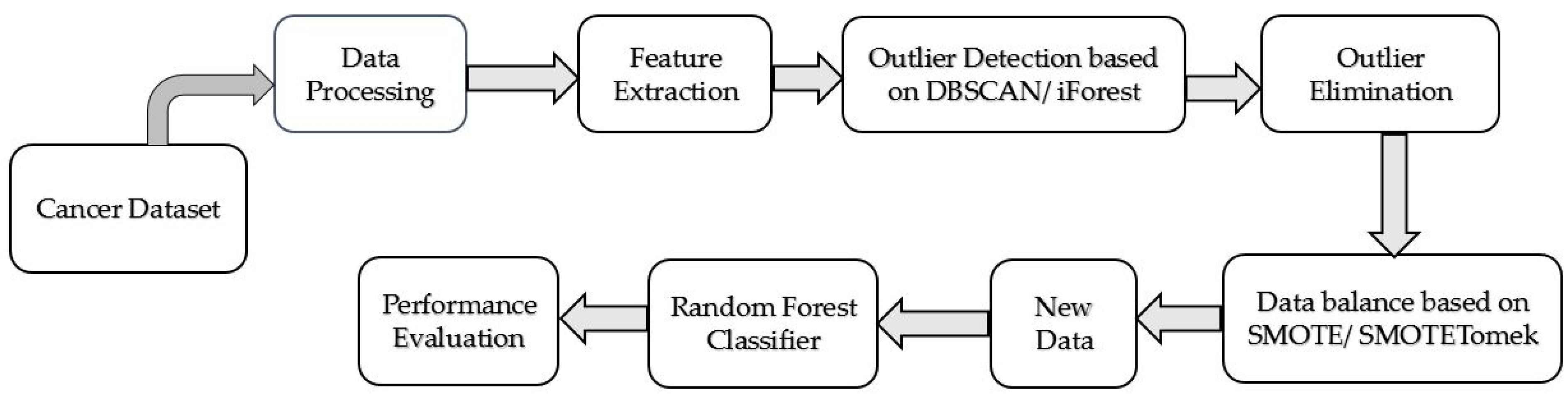
The proposed CCPM consists of outlier detection based on DBSCAN and iForest. It also has SMOTE and SMOTETomek to balance the data with RF for cancer prediction.
Lastly, the performance of the proposed CCPM is compared with the performances of other existing models. Figure 1 elucidates the proposed CCPM model.
We used 70 % dataset values for training and 30% for testing with 10 cross validation. We have used the Python programming language and scikit-learn, pandas, numpy libraries used for machine learning models. For outlier detection, we have used scikit-learn library in python programming language [73]. For oversampling, we have used the imbalanced-learn Python library [74].
3.2. Evaluation Metrics
The prediction output may have the following four possible outcomes on the basis of a confusion matrix [75], true positive (TP), true negative (TN), false positive (FP), and false negative (FN). Table 2 displays the precision, recall, specificity, F1 score, and accuracy. Table 3 shows different outcomes of two-class prediction.
4. Results and Discussion
This section deals with the results of feature extraction and four scenarios of CCPM in terms of precision, sensitivity, specificity, F1 score, and accuracy. Four scenarios are divided into four sections. Each section displays results and their explanation. We then compared biopsy results with results of past studies and some practical implications to conclude this section.
4.1. Feature Extraction Results
In the present study, we used chi-square to extract the features from the dataset. The main aim of the feature extraction technique is to extract the most valuable features from a given rather than the whole features. For simplicity, we have extracted first ten features that have the highest chi-score. Besides, we have added the chi-score of ten variables in the feature extraction table. We used these features for our analysis. After selecting these features, we used outlier detection techniques to remove outliers from the data. Table 4 displays the results of chi-square.
4.2. DBSCAN and iForest for Outlier Detection
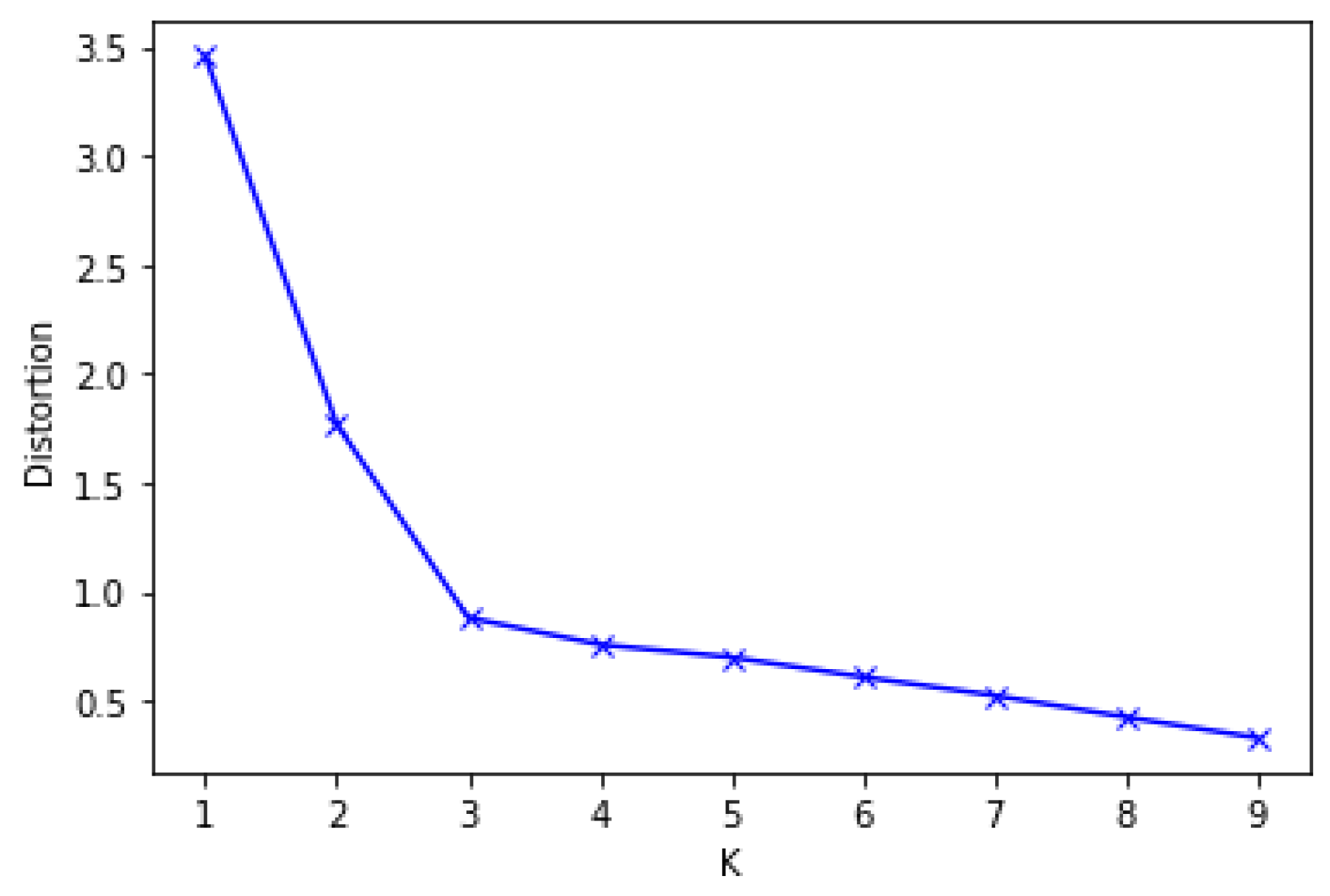
To implement the DBSCAN-based outlier detection, the optimum value of MinPts and eps must first be established. If the value of eps is too low, it will generate more clusters and normal data may be counted as outliers. On the other hand, if it is too large, it will produce fewer clusters, and true outliers could be categorized as normal data [23,43,44]. We specified the MinPts value to be 5. Next, we have to determine the optimal number of eps. First, we measure each point’s average distance from its nearest neighbors. The value k represents MinPts and is outlined by the user. The goal is to decide the “knee” used to estimate the parameter collection of eps. A “knee” is the point at which a sharp shift occurs along the k-distance curve [46]. Figure 2 displays the k-dist graph sorted for the cervical cancer data set and the optimal value of eps. The "knee" shows up at the distance of 3 in the cervical cancer dataset. Lastly, the outlier data are excluded, and standard data are used for further analysis.
iForest works in two phases. The first (training) stage constructs isolation trees using training set subsamples. The second stage (testing) passes through isolation trees to obtain an outlier score for each case. Both subsample size (MaxSample) and number of trees to be built (NumTree) are essential parameters to be calculated. The iForest works well when the MaxSample is kept small; the larger MaxSample reduces the ability of iForest to isolate outer data, as normal data can meddle with isolation [48,49,50]. Number of Trees influences the scale of the ensemble. We tried different configuration parameters and found that MaxSample is 10% of the total data size and NumTree is 100% optimal. The iForest was implemented using scikit-learn python library. In case of DBSCAN, we found two outliers. We removed these outliers and processed the data for further analysis. However, iForest found eighty-six outliers. We removed those outliers as well and processed the data.
4.3. SMOTE and SMOTETomek for Balancing the Dataset
We also used over-sampling methods to increase the number of cases in a balanced way. We applied SMOTE or SMOTETomek methods to balance the datasets. SMOTE oversamples the minority class to randomly generate instances and increase minority class instances, and Tomek under-samples a class to remove noise while maintaining balanced distributions. As can be seen in Table 5, the dataset is balanced after the application of SMOTE and SMOTETomek. The classification aim is to diminish errors during the learning process; hence, we anticipate that a better model accuracy can be attained from the balanced datasets.
4.4. Results of Target Variables: Biopsy, Schiller, Hinselmann, Cytology
The ten features extracted by Chi-square were used for all models (SVM, multilayer perceptron (MLP), logistic regression (LR), naïve Bayes, and K-nearest neighbors (KNN)), and all four target variables (Biopsy, Schiller, Hinselmann, and Cytology). For each of the target variables, the CCPM was compared with other conventional machine learning models. The results of CCPM for each of the target variables outperformed previous machine learning approaches (with reference to Table 6, Table 7, Table 8, Table 9, Table 10, Table 11, Table 12, Table 13, Table 14, Table 15, Table 16, Table 17, Table 18, Table 19, Table 20 and Table 21). The key reason for these results is the combination of the outlier removal and data balancing techniques. Hence, this improves the accuracy for our CCPM.
4.5. Comparison with Previous Studies
We compared the results of our CCPM with past studies that used the cervical cancer dataset. The study by Wu and Zhu [10] used SVM-RFE and SVM-PCA, while Abdoh et al. [22] used SMOTE-RF-RFE and SMOTE-RF-PCA. Table 22, Table 23, Table 24 and Table 25 illustrates the comparison of results on the sensitivity, specificity, and accuracy of all target variables of CCPM with Wu and Zhu [10] and Abdoh et al. [22]. All four proposed scenarios of CCPM surpassed past studies by Wu and Zhu [10] and Abdoh et al. [22] in terms of sensitivity, specificity, and accuracy. A study by Deng et al. [76] used SMOTE for handling the imbalanced data, and SVM, XGBoost and RF to identify the risk factors of cervical cancers. Our CCPM produces better results as compared to the Deng et al. [76]. They accuracies achieved by SVM, XGBoostand Random Forest are 90.34, 96.34, and 97.39, respectively. A recent study by Adem et al. [20] used a stacked autoencoder with a soft-max layer and achieved an accuracy of 97.25% in the cervical cancer dataset. Our CCPM surpassed Deng et al. [76] and Adem et al. [20] in terms of accuracy. Thus, we can conclude that our proposed CCPM is better than other machine learning models as well as past studies.
Our proposed CCPM has four combinations, two outlier detection methods and two data oversampling methods, and their results varied target variables and performance measures. For example, the combination of iForest and SMOTETomek showed the best performances in sensitivity and accuracy in biopsy and specificity in Schiller and Hinselmann, but that of DBSCAN and SMOTE was the best in sensitivity and accuracy in Schiller and Hinselmann tests. In summary, iForest showed better results than DBSCAN for biopsy tests, but DBSCAN was usually better than iForest for the cytology test. However, we recommend using all of four combinations for predicting cervical cancer and using ensemble results of them for more robust prediction.
In case of risk factors, Table 1 showed the entire attributes’ name and the corresponding number of each attribute. The ten features in our study were Smokes (years), Hormonal Contraceptives (years), STDs (number), STDs: genital herpes, STDs: HIV, STDs: Number of diagnosis, Dx: Cancer, Dx: HPV, Dx. We compared the results of risk factors based on feature extraction results with past studies [10,22,77]. The factor Dx: Cancer found in our study is also validated by the Wu and Zhu [10], while the factors smokes per years and Hormonal contraceptives found by Wu and Zhu [10], and Smokes and Hormonal Contraceptives found by Abdoh et al. [22] seemed quite relevant to the factors Smokes (years) and Hormonal Contraceptives (years) factors found in the present study. Furthermore, we compared our features result with past study by Nithya and Ilango [77]. These findings have revealed that the common features between both studies include Smokes (years), Hormonal Contraceptives (years), STDs: Number of diagnosis, Dx: Cancer, Dx: HPV, and Dx. Hence, Smokes (years), Hormonal Contraceptives (years), STDs: Number of diagnosis, Dx: Cancer, Dx: HPV, and Dx are the factors that corresponds to the riskiest factors of cervical cancer. Based on our experiment the existence of these factors enhances the risk of being a cervical cancer patient. The present work identified the topmost significant features for the classification of cervical cancer patients to be Smokes (years), Hormonal Contraceptives (years), STDs: Number of diagnosis, Dx: Cancer, Dx: HPV, and Dx.
The complexity of an algorithm is generally calculated using Big-O notation [78,79,80]. Time complexity and space complexity are two types of computational complexity [81,82]. Time complexity deals with how long the algorithm is executed for, while space complexity deals with how much memory is used by its algorithm. An algorithm will process amounts of data, where N is a symbol of amounts of data. If an algorithm does not depend on N, then the algorithm has constant complexity or symbolized by O(1) (Big-O one). On the contrary, if the algorithm is dependent on N, the complexity depends on line code in algorithm and it is can be O(n), O(n2), O(log n) and others. Let n be the number of training examples, d be the number of dimensions of the data, k be the number of neighbors or the number of trees, and c be the number of classes. Table 26 depicts the time and space complexities of some machine learning algorithms. In our CCPM, the RF becomes slow and requires more memory space for training as compared to other algorithms. In addition, the proposed CCPM requires additional computation for outlier detection and data balancing. In our CCPM, however, we got better accuracy compared to other conventional machine learning methods.
4.6. Practical Implications
Lee et al. [83] have studied the impacts of educational text messages concerning HPV vaccination and its advantages and observed a substantial upsurge in HPV vaccination intake in targeted populations. Cancer screening programs have also used text messaging in an attempt to tackle the screening intake. Weaver et al. [84] have recently examined how elderly patients would be interested in text messages intended to motivate their participation in a screening program. Their findings indicated that older populations were extremely interested in such messages based on their involvement. A recent study by Ijaz et al. [46] has used IoT for a healthcare monitoring system for patients at home and used personal healthcare devices that perceive and estimate a persons’ biomedical signals. The system can notify health personnel in real-time when patients experience emergency situations.
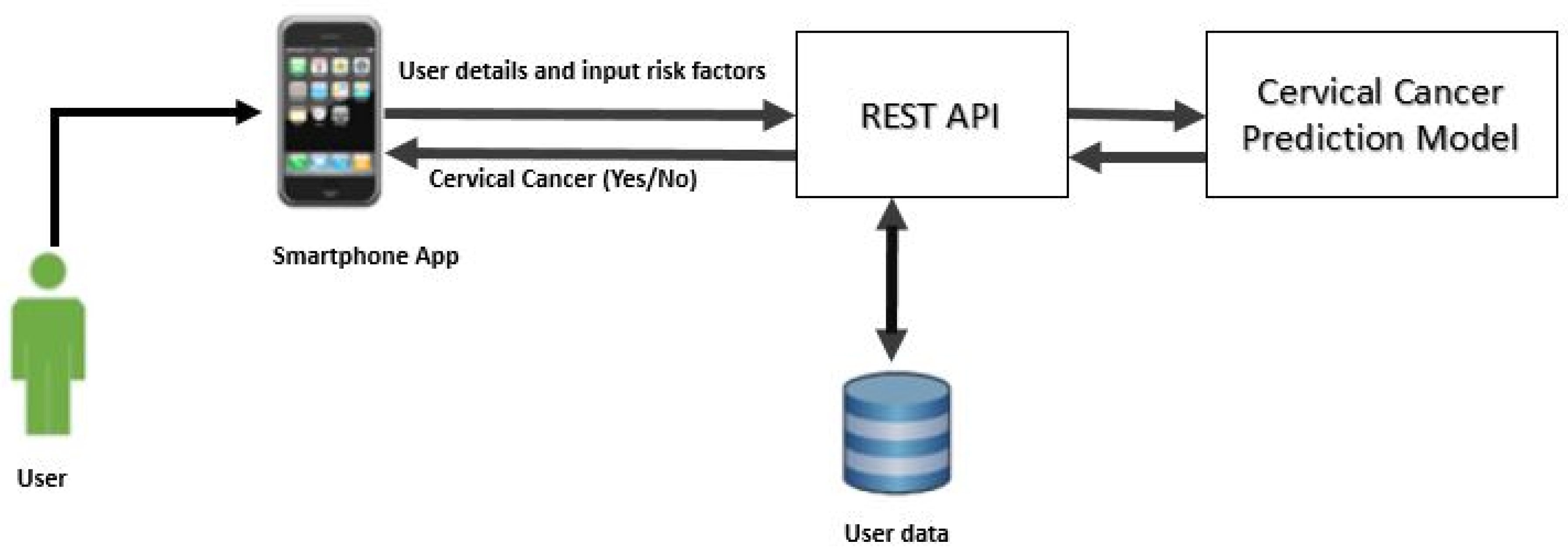
In the present work, we implemented CCPM into a mobile app to show its practical implication for simple users. Figure 3 shows the architecture framework of CCPM. A mobile app collects user’s risk factor data and then sends it to Representational State Transfer (REST API) to be stored in a a secure remote server. We used NoSQL MongoDB to store user data by keeping in mind that it could store large amounts of data. Finally, CCPM was used to forecast the presence of cervical cancer as long as users input risk factors. Predication results are shown in the mobile app.
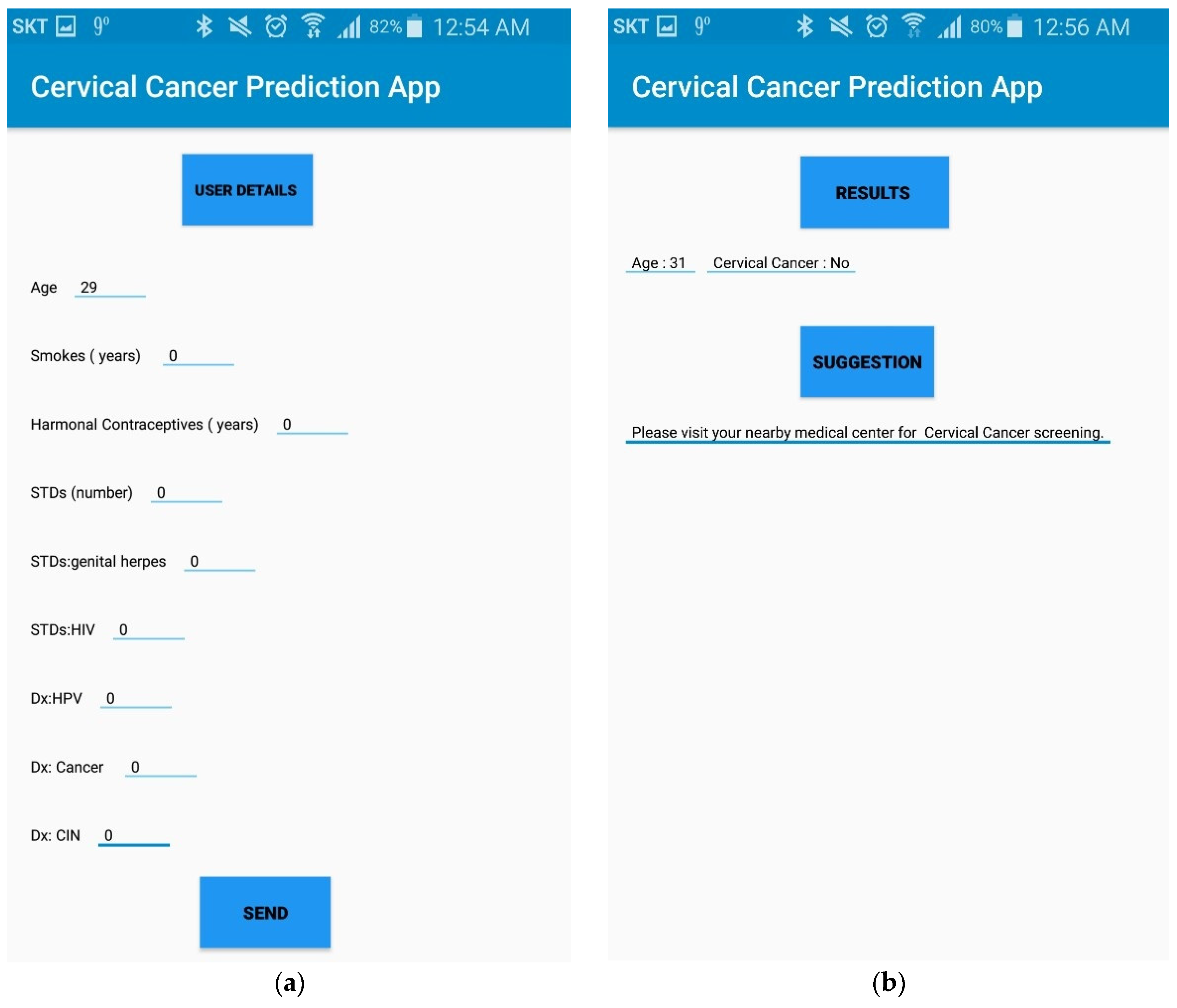
Figure 4a,b shows a prototype of the mobile app. When a user presses the “send” button, risk factors that the user inputs are stored in the remote server. CCPM is then activated to foresee the existence of cervical cancer. Figure 4b depicts the interface of mobile application when the user receives prediction results. Therefore, it is expected that the CCPM mobile application can help users find the risk of cervical cancer proficiently at an early stage.
In our CCPM mobile application, maintaining the safety of healthcare data is of paramount importance. The data in the CCPM mobile application are encrypted. Encryption is an essential for our CCPM mobile application since it scrambles a user’s personal data. We used secure sockets layer (SSL) technology that encrypts information transmitted between a mobile application and the server. SSL uses a cryptographic system that uses two keys to encrypt data, e.g., a public key known to everyone and a private or secret key known only to the recipient of the message [85,86]. The NoSQL MongoDB helps to store the user data. A secure log-in feature can be added to mobile application which is called two-factor authentication (2FA). 2FA improves the mobile application’s security. Some examples of 2FA include: Username/password + SMS code, Username/password + code sent via email, and Username/password + biometric authentication (a fingerprint). Another important feature to secure the user data is with the help of data wiping. To implement data wiping, an app can: log out a user after a certain period of inactivity, keep information in an encrypted form, and perform an automatic data wipe after a certain number of unsuccessful login attempts. This gives users a sense of greater control over privacy, security, and confidentiality in towards their healthcare data. The security systems described above can keep the health data secured and safe in our mobile application.
5. Conclusions
As indicated by the World Health Organization (WHO), about 80% cases of cervical cancer are noted in developing nations. A cure ratio is described as the ratio of female cases that are healed from the disease. It can be boosted by classifying the risk factors of cervical cancer [22]. This study proposed a CCPM that used Chi-square as feature extraction technique. We extracted ten features and used them in our study. The current dataset is unbalanced. It has a lot of missing values. For missing values, we used mean equation. The current work proposed CCPM by joining DBSCAN and iForest for outlier detection, with SMOTE and SMOTETomek for class balancing and RF as a classifier. The CCPM can help users find the risk of cervical cancer at an early stage. Accuracies achieved by Biopsy forDBSCAN + SMOTETomek + RF, DBSCAN + SMOTE+ RF, iForest + SMOTETomek + RF, and iForest + SMOTE + RF were 96.708%, 97.007%, 98.919%, and 98.925%, respectively. While for Schiller accuracies for DBSCAN + SMOTETomek + RF, DBSCAN + SMOTE+ RF, iForest + SMOTETomek + RF, iForest + SMOTE + RF were 99.48%, 99.22%, 98.50%, and 98.71% respectively. In case of Hinselmann, the accuracies achieved by DBSCAN + SMOTETomek + RF, DBSCAN + SMOTE+ RF, iForest + SMOTETomek + RF, iForest + SMOTE + RF were 99.50%, 99.01%, 99.50%, and 99.50% respectively. For Cytology, the accuracies achieved by DBSCAN + SMOTETomek + RF, DBSCAN + SMOTE+ RF, iForest + SMOTETomek + RF, iForest + SMOTE + RF were 97.72%, 97.22%, 97.50%, and 97.51% respectively. Hence, combining iForest with SMOTE and SMOTETomek can produce better results than combining DBSCAN with SMOTE and SMOTETomek. Besides, we compared Hinselmann, Schiller, Cytology, and Biopsy results with past studies by Wu and Zhu [10] and Abdoh et al. [22] in terms of sensitivity, specificity, and accuracy. Our results revealed that DBSCAN + SMOTETomek + RF, DBSCAN + SMOTE+ RF, iForest + SMOTETomek + RF, iForest + SMOTE + RF surpassed past studies by Wu and Zhu [10] and Abdoh et al. [22]. Besides, Our CCPM surpassed Deng et al. [76] and Adem et al. [20] in terms of accuracy. As a result, we can conclude that our proposed CCPM is better than other models as well as past studies.
In future work, we will employ more diverse techniques for outlier detection and over-sampling methods. We will also apply each combination to CCPM to improve its diagnosis performance. The proposed method can be applied to other cervical cancer datasets. Results on these may provide additional intuitions for the early diagnosis of cervical cancer.
This study also has a limitation, as only one dataset is employed. Since we only focus on cervical cancer in this study, we only used one dataset. In future research, the proposed CCPM can be applied to diverse cancer datasets (such as breast, liver, lung, prostate, thyroid, and kidney) to enhance the clarity and quality of results. Another limitation is that our algorithm (which is a combination of outlier technique and data balancing with RF) becomes slower and needs more memory to run, but as we got a better accuracy, it serves our purpose.
Author Contributions
Y.S. conceived and designed the experiments; M.F.I. performed the experiments; M.F.I. and M.A. analyzed the data; M.F.I. wrote the paper. All authors have read and agreed to the published version of the manuscript.
Data Availability
The data used in present study is publicly available at the given link by UCI machine leaning repository. https://archive.ics.uci.edu/ml/datasets/Cervical+cancer+%28Risk+Factors%29.
Funding
Muhammad Fazal Ijaz and Youngdoo Son were supported by National Research Foundation of Korea (NRF) grant funded by the Korea government (MSIT) (Nos. 2017R1E1A1A03070102; 2020R1C1C1003425). Muhammad Attique was supported by the National Research Foundation of Korea grant funded by the Korean Government (2020R1G1A1013221).
Conflicts of Interest
The authors declare no conflict of interest.
References
- Yang, X.; Da, M.; Zhang, W.; Qi, Q.; Zhang, C.; Han, S. Role of lactobacillus in cervical cancer. Cancer Manag. Res. 2018, 10, 1219–1229. [Google Scholar] [CrossRef] [PubMed] [Green Version]
- Fitzmaurice, C.; Dicker, D.; Pain, A.; Hamavid, H.; Moradi-Lakeh, M.; MacIntyre, M.F.; Allen, C.; Hansen, G.; Woodbrook, R.; Wolfe, C.; et al. The global burden of cancer 2013. JAMA. Oncol. 2015, 1, 505–527. [Google Scholar] [CrossRef] [PubMed]
- Seo, S.-S.; Oh, H.Y.; Lee, J.-K.; Kong, J.-S.; Lee, D.O.; Kim, M.K. Combined effect of diet and cervical microbiome on the risk of cervical intraepithelial neoplasia. Clin. Nutr. 2016, 35, 1434–1441. [Google Scholar] [CrossRef] [PubMed]
- Suehiro, T.T.; Malaguti, N.; Damke, E.; Uchimura, N.S.; Gimenes, F.; Souza, R.P.; da Silva, V.R.S.; Consolaro, M.E.L. Association of human papillomavirus and bacterial vaginosis with increased risk of high-grade squamous intraepithelial cervical lesions. Int. J. Gynecol. Cancer 2019, 29, 242–249. [Google Scholar] [CrossRef]
- Khan, I.; Nam, M.; Kwon, M.; Seo, S.-S.; Jung, S.; Han, J.S.; Hwang, G.-S.; Kim, M.K. LC/MS-based polar metabolite profiling identified unique biomarker signatures for cervical cancer and cervical intraepithelial neoplasia using global and targeted metabolomics. Cancers 2019, 11, 511. [Google Scholar] [CrossRef] [Green Version]
- Luhn, P.; Walker, J.; Schiffman, M.; Zuna, R.E.; Dunn, S.T.; Gold, M.A.; Smith, K.; Mathews, C.; Allen, R.A.; Zhang, R.; et al. The role of co-factors in the progression from human papillomavirus infection to cervical Cancer. Gynecol. Oncol. 2013, 128, 265–270. [Google Scholar] [CrossRef] [Green Version]
- Cervical Cancer Prevention. 2015. Available online: https://www.Cancergov/types/cervical/hp/cervical-prevention-pdq (accessed on 22 April 2020).
- Exner, M.; Kühn, A.; Stumpp, P.; Höckel, M.; Horn, L.C.; Kahn, T.; Brandmaier, P. Value of diffusion-weighted MRI in diagnosis of uterine cervical cancer: A prospective study evaluating the benefits of DWI compared to conventional MR sequences in a 3T environment. Acta. Radiol. 2016, 57, 869–877. [Google Scholar] [CrossRef]
- McVeigh, P.Z.; Syed, A.M.; Milosevic, M.; Fyles, A.; Haider, M.A. Diffusion-weighted MRI in cervical Cancer. Eur. Radiol. 2008, 18, 1058–1064. [Google Scholar] [CrossRef]
- Wu, W.; Zhou, H. Data-driven diagnosis of cervical cancer with support vector machine-based approaches. IEEE Access 2017, 5, 25189–25195. [Google Scholar] [CrossRef]
- Yang, J.; Nolte, F.S.; Chajewski, O.S.; Lindsey, K.G.; Houser, P.M.; Pellicier, J.; Wang, Q.; Ehsani, L. Cytology and high risk HPV testing in cervical cancer screening program: Outcome of 3-year follow-up in an academic institute. Diagn. Cytopathol. 2018, 46, 22–27. [Google Scholar] [CrossRef]
- Cibula, D.; Pötter, R.; Planchamp, F.; Avall-Lundqvist, E.; Fischerova, D.; Meder, C.H.; Köhler, C.; Landoni, F.; Lax, S.; Lindegaard, J.C.; et al. The European society of Gynaecological Oncology/European society for radiotherapy and Oncology/European society of pathology guidelines for the management of patients with cervical cancer. Int. J. Gynecol. Cancer 2018, 28, 641–655. [Google Scholar] [CrossRef] [PubMed]
- Shi, P.; Zhang, L.; Ye, N. Sfterummetabolomic analysis of cervical cancer patients by gas chromatography-mass spectrometry. Asian J. Chem. 2015, 27, 547–551. [Google Scholar]
- Ghoneim, A.; Muhammad, G.; Hossain, M.S. Cervical cancer classification using convolutional neural networks and extreme learning machines. Future Gener. Comp. Syst. 2020, 102, 643–649. [Google Scholar] [CrossRef]
- Chandran, K.P.; Kumari, U.V.R. Improving cervical cancer classification on MR images using texture analysis and probabilistic neural network. Int. J. Sci. Eng. Technol. Res. 2015, 4, 3141–3145. [Google Scholar]
- Malli, P.K.; Nandyal, S. Machine learning technique for detection of cervical cancer using k-NN and artificial neural network. Int. J. Emerg. Trends Technol. Comput. Sci. 2017, 6, 145–149. [Google Scholar]
- Gupta, R.; Sarwar, A.; Sharma, V. Screening of cervical cancer by artificial intelligence based analysis of digitized papanicolaou-smear images. Int. J. Contemp. Med. Res. 2017, 4, 1108–1113. [Google Scholar]
- Zhang, L.; Lu, L.; Nogues, I.; Summers, R.M.; Liu, S.; Yao, J. DeepPap: Deep convolutional networks for cervical cell classification. IEEE J. Biomed. Health Inform. 2017, 21, 1633–1643. [Google Scholar] [CrossRef] [Green Version]
- Bora, K.; Chowdhury, M.; Mahanta, L.B.; Kundu, M.K.; Das, A.K. Pap smear image classification using convolutional neural network. In Proceedings of the Tenth Indian Conference on Computer Vision, Graphics and Image Processing, Bangalore, India, 18–22 December 2016; pp. 1–8. [Google Scholar]
- Adem, K.; Kilicarslan, S.; Comert, O. Classification and diagnosis of cervicalcancer with softmax classification with stacked autoencoder. Expert Syst. Appl. 2019, 115, 557–564. [Google Scholar] [CrossRef]
- Kourou, K.; Exarchos, T.P.; Exarchos, K.P.; Karamouzis, M.V.; Fotiadis, D.I. Machine learning applications in cancer prognosis and prediction. Comput. Struct. Biotechnol. 2015, 13, 8–17. [Google Scholar] [CrossRef] [Green Version]
- Abdoh, S.F.; Rizka, M.A.; Maghraby, F.A. Cervical cancer diagnosis using random forest classifier with SMOTE and feature reduction techniques. IEEE. Access 2018, 6, 59475–59485. [Google Scholar] [CrossRef]
- Ester, M.; Kriegel, H.P.; Jörg, S.; Xu, X. A density-based algorithm for discovering clusters in large spatial databases with noise. In Proceedings of the 2nd International Conference on Knowledge Discovery and Data Mining, IAAI, Portland, OR, USA, 2–4 August 1996; pp. 226–231. [Google Scholar]
- Chawla, N.V.; Bowyer, K.W.; Hall, L.O.; Kegelmeyer, W.P. SMOTE: Synthetic minority over-sampling technique. J. Artif. Intell. Res. 2002, 16, 321–357. [Google Scholar] [CrossRef]
- Sanguanmak, Y.; Hanskunatai, A. (2016, July). DBSM: The combination of DBSCAN and SMOTE for imbalanced data classification. In Proceedings of the 2016 13th International Joint Conference on Computer Science and Software Engineering (JCSSE), Khon Kaen, Thailand, 13–15 July 2016; pp. 1–5. [Google Scholar]
- Zhang, L.; Kong, H.; Chin, C.T.; Liu, S.; Fan, X.; Wang, T.; Chen, S. Automation-assisted cervical cancer screening in manual liquid-based cytology with hematoxylin and eosin staining. Cytom. Part A 2014, 85, 214–230. [Google Scholar] [CrossRef] [PubMed]
- Vink, J.P.; Van Leeuwen, M.B.; Van Deurzen, C.H.M.; De Haan, G. Efficient nucleus detector in histopathology images. J. Microsc. 2013, 249, 124–135. [Google Scholar] [CrossRef] [PubMed] [Green Version]
- Tareef, A.; Song, Y.; Cai, W.; Huang, H.; Chang, H.; Wang, Y.; Fulham, M.; Feng, D.; Chen, M. Automatic segmentation of overlapping cervical smear cells based on local distinctive features and guided shape deformation. Neurocomputing 2017, 221, 94–107. [Google Scholar] [CrossRef]
- Ragothaman, S.; Narasimhan, S.; Basavaraj, M.G.; Dewar, R. Unsupervised segmentation of cervical cellimages using gaussian mixture model. In Proceedings of the IEEE Conference on Computer Vision and Pattern Recognition Workshops, Las Vegas, NV, USA, 26 June–1 July 2016; pp. 70–75. [Google Scholar]
- Zhao, L.; Li, K.; Wang, M.; Yin, J.; Zhu, E.; Wu, C.; Wang, S.; Zhu, C. Automatic cytoplasm and nuclei segmentation for color cervical smear image using an efficient gap-search MRF. Comput. Biol. Med. 2016, 71, 46–56. [Google Scholar] [CrossRef] [PubMed]
- Tareef, A.; Song, Y.; Cai, W.; Feng, D.D.; Chen, M. Automated three-stage nucleus and cytoplasmsegmentation of overlapping cells. In Proceedings of the 2014 13th International Conference on Control Automation Robotics & Vision (ICARCV), Singapore, 10–12 December 2014; pp. 865–870. [Google Scholar]
- Tseng, C.J.; Lu, C.J.; Chang, C.C.; Chen, G.D. Application of machine learning to predict the recurrence-proneness for cervical Cancer. Neural. Comput. Appl. 2014, 24, 1311–1316. [Google Scholar]
- Hu, B.; Tao, N.; Zeng, F.; Zhao, M.; Qiu, L.; Chen, W.; Tan, Y.; Wei, Y.; Wu, X.; Wu, X. A risk evaluation model of cervical cancer based on etiology and human leukocyte antigen allele susceptibility. Int. J. Infect. Dis. 2014, 28, 8–12. [Google Scholar] [CrossRef] [Green Version]
- Sharma, S. Cervical cancer stage prediction using decision tree approach of machine learning. Int. J. Adv. Res. Comput. Commun. Eng. 2016, 5, 345–348. [Google Scholar]
- Sobar, S.; Machmud, R.; Wijaya, A. Behavior determinant based cervical cancer early detection with machine learning algorithm. Adv. Sci. Lett. 2016, 22, 3120–3123. [Google Scholar] [CrossRef]
- Le Thi, H.A.; Le, H.M.; Dinh, T.P. Feature selection in machine learning: An exact penalty approach using a difference of convex function algorithm. Mach. Learn. 2015, 101, 163–186. [Google Scholar] [CrossRef]
- Rehman, O.; Zhuang, H.; Muhamed Ali, A.; Ibrahim, A.; Li, Z. Validation of miRNAs as breast cancer biomarkers with a machine learning approach. Cancers 2019, 11, 431. [Google Scholar] [CrossRef] [PubMed]
- Jin, X.; Xu, A.; Bie, R.; Guo, P. Machine learning techniques and chi-square feature selection for cancerclassification using SAGE gene expression profiles. Lect. Notes Comput. Sci. 2006, 3916, 106–115. [Google Scholar]
- Rouzbahani, H.K.; Daliri, M.R. Diagnosis of Parkinson’s disease in human using voice signals. Basic Clin. Neurosci. 2011, 2, 12–20. [Google Scholar]
- Musa, P.; Sen, B.; Delen, D. Computer-aided diagnosis of Parkinson’s disease using complex-valued neural networks and mRMR feature selection algorithm. J. Healthc. Eng. 2015, 6, 281–302. [Google Scholar]
- Sicong, K.; Davison, B.D. Learning word embeddings with chi-square weights for healthcare tweet classification. Appl. Sci. 2017, 7, 846. [Google Scholar]
- Hao, S.; Zhou, X.; Song, H. A new method for noise data detection based on DBSCAN and SVDD. In Proceedings of the 2015 IEEE International Conference on Cyber Technology in Automation, Control, and Intelligent Systems (CYBER), Shenyang, China, 8–12 June 2015; pp. 784–789. [Google Scholar]
- ElBarawy, Y.M.; Mohamed, R.F.; Ghali, N.I. Improving social network community detection using DBSCAN algorithm. In Proceedings of the 2014 World Symposium on Computer Applications & Research (WSCAR), Sousse, Tunisia, 18–20 January 2014; pp. 1–6. [Google Scholar]
- Abid, A.; Kachouri, A.; Mahfoudhi, A. Outlier detection for wireless sensor networks using density-based clustering approach. IET Wirel. Sens. Syst. 2017, 7, 83–90. [Google Scholar] [CrossRef]
- Tian, H.X.; Liu, X.J.; Han, M. An outlier’s detection method of time series data for soft sensor modeling. In Proceedings of the 2016 Chinese Control and Decision Conference (CCDC), Yinchuan, China, 28–30 May 2016; pp. 3918–3922. [Google Scholar]
- Ijaz, M.F.; Alfian, G.; Syafrudin, M.; Rhee, J. Hybrid prediction model for type 2 diabetes and hypertension using dbscan-based outlier detection, synthetic minority over sampling technique (SMOTE), and random forest. Appl. Sci. 2018, 8, 1325. [Google Scholar] [CrossRef] [Green Version]
- Verbiest, N.; Ramentol, E.; Cornelis, C.; Herrera, F. Preprocessing noisy imbalanced datasets using SMOTE enhanced with fuzzy rough prototype selection. Appl. Soft. Comput. 2014, 22, 511–517. [Google Scholar] [CrossRef]
- Liu, F.T.; Ting, K.M.; Zhou, Z.H. Isolation Forest. In Proceedings of the 2008 Eighth IEEE International Conference on Data Mining, Pisa, Italy, 15–19 December 2008; pp. 413–422. [Google Scholar]
- Liu, F.T.; Ting, K.M.; Zhou, Z.H. Isolation-based anomaly detection. ACM Trans. Knowl. Discov. Data 2012, 6, 1–39. [Google Scholar] [CrossRef]
- Domingues, R.; Filippone, M.; Michiardi, P.; Zouaoui, J. A comparative evaluation of outlier detection algorithms: Experiments and analyses. Pattern Recognit. 2018, 74, 406–421. [Google Scholar] [CrossRef]
- Calheiros, R.N.; Ramamohanarao, K.; Buyya, R.; Leckie, C.; Versteeg, S. On the effectiveness of isolation-based anomaly detection in cloud data centers. Concurr. Comput. Pract. Eng. 2017, 29, 4169. [Google Scholar] [CrossRef]
- Bauder, R.; da Rosa, R.; Khoshgoftaar, T. Identifying Medicare Provider Fraud with Unsupervised Machine Learning. In Proceedings of the 2018 IEEE International Conference on Information Reuse and Integration (IRI), Salt Lake City, UT, USA, 6–9 July 2018; pp. 285–292. [Google Scholar]
- Lorenzo, M.; Susto, G.A.; del Favero, S. Detection of insulin pump malfunctioning to improve safety in artificial pancreas using unsupervised algorithms. J. Diabetes Sci. Technol. 2019, 13, 1065–1076. [Google Scholar]
- Meneghetti, L.; Terzi, M.; del Favero, S.; Susto, G.A.; Cobelli, C. Data-driven anomaly recognition for unsupervised model-free fault detection in artificial pancreas. IEEE Trans. Control. Syst. Technol. 2020, 28, 33–47. [Google Scholar] [CrossRef]
- Dos Santos, H.D.P.; Ulbrich, A.H.D.P.S.; Woloszyn, V.; Vieira, R. DDC-Outlier: Preventing medication errors using unsupervised learning. IEEE J. Biomed. Health Inform. 2019, 23, 874–881. [Google Scholar] [CrossRef] [PubMed]
- Cheng, W.; Zhu, W. Predicting 30-Day Hospital Readmission for Diabetics Based on Spark. In Proceedings of the 2019 3rd International Conference on Imaging, Signal Processing and Communication (ICISPC), Singapore, 27–29 July 2019; pp. 125–129. [Google Scholar]
- Kurnianingsih; Nugroho, L.E.; Widyawan; Lazuardi, L.; Prabuwono, A.S. Detection of Anomalous Vital Sign of Elderly Using Hybrid K-Means Clustering and Isolation Forest. In Proceedings of the TENCON 2018—2018 IEEE Region 10 Conference, Jeju, Korea, 28–31 October 2018; pp. 913–918. [Google Scholar]
- Fallahi, A.; Jafari, S. An expert system for detection of breast cancer using data preprocessing and Bayesian network. Int. J. Adv. Sci. Technol. 2011, 34, 65–70. [Google Scholar]
- Wang, K.-J.; Makond, B.; Chen, K.-H.; Wang, K.-M. A hybrid classifier combining SMOTE with PSO to estimate 5-year survivability of breast cancer patients. Appl. Soft Comput. 2014, 20, 15–24. [Google Scholar] [CrossRef]
- Santos, M.S.; Abreu, P.H.; García-Laencina, P.J.; Simão, A.; Carvalho, A. A new cluster-based oversampling method for improving survival prediction of hepatocellular carcinoma patients. J. Biomed. Inform. 2015, 58, 49–59. [Google Scholar] [CrossRef] [Green Version]
- Batista, G.E.; Prati, R.C.; Monard, M.C. A study of the behavior of several methods for balancing machine learning training data. ACM SIGKDD Explor. Newslett. 2004, 6, 20–29. [Google Scholar] [CrossRef]
- Goel, G.; Maguire, L.; Li, Y.; McLoone, S. Evaluation of Sampling Methods for Learning from Imbalanced Data. In Intelligent Computing Theories; Springer: Berlin/Heidelberg, Germany, 2013; pp. 392–401. [Google Scholar]
- Chen, T.; Shi, X.; Wong, Y.D. Key feature selection and risk prediction for lane-changing behaviors based on vehicles’ trajectory data. Accid. Anal. Prev. 2019, 129, 156–169. [Google Scholar] [CrossRef]
- Yan, Y.; Liu, R.; Ding, Z.; Du, X.; Chen, J.; Zhang, Y. A parameter-free cleaning method for smote in imbalanced classification. IEEE Access 2019, 7, 23537–23548. [Google Scholar] [CrossRef]
- Son, L.H.; Baik, S. A robust framework for self-care problem identification for children with disability. Symmetry 2019, 11, 89. [Google Scholar]
- Teixeira, V.; Camacho, R.; Ferreira, P.G. Learning influential genes on cancer gene expression data with stacked denoising autoencoders. In Proceedings of the 2017 IEEE International Conference on Bioinformatics and Biomedicine (BIBM), Kansas City, MO, USA, 13–16 November 2017; pp. 1201–1205. [Google Scholar]
- Zeng, M.; Zou, B.; Wei, F.; Liu, X.; Wang, L. Effective prediction of three common diseases by combining SMOTE with Tomek links technique for imbalanced medical data. In Proceedings of the 2016 IEEE International Conference of Online Analysis and Computing Science (ICOACS), Chongqing, China, 28–29 May 2016; pp. 225–228. [Google Scholar]
- Kabir, M.F.; Ludwig, S. Classification of Breast Cancer Risk Factors Using Several Resampling Approaches. In Proceedings of the 17th IEEE International Conference on Machine Learning and Applications (ICMLA), Orlando, FL, USA, 17–20 December 2018; pp. 1243–1248. [Google Scholar]
- Mohan, A.; Rao, M.D.; Sunderrajan, S.; Pennathur, G. Automatic classification of protein structures using physicochemical parameters. Interdiscip. Sci. Comput. Life Sci. 2014, 6, 176–186. [Google Scholar] [CrossRef] [PubMed]
- Seera, M.; Lim, C.P. A hybrid intelligent system for medical data classification. Expert Syst. Appl. 2014, 41, 2239–2249. [Google Scholar] [CrossRef]
- Fernandes, K.; Cardoso, J.S.; Fernandes, J. Transfer learning with partial observability applied to cervical cancer screening. In Iberian Conference on Pattern Recognition and Image Analysis; Springer: Cham, Switzerland, 2017; pp. 243–250. [Google Scholar]
- Wright, T.C., Jr. Chapter 10: Cervical cancer screening using visualization techniques. JNCI Monogr. 2003, 31, 66–71. [Google Scholar] [CrossRef] [PubMed]
- Pedregosa, F.; Varoquaux, G.; Gramfort, A.; Michel, V.; Thirion, B.; Grisel, O.; Blondel, M.; Prettenhofer, P.; Weiss, R.; Dubourg, V.; et al. Scikit-learn: Machine learning in Python. J. Mach. Learn. Res. 2011, 12, 2825–2830. [Google Scholar]
- Lemaître, G.; Nogueira, F.; Aridas, C.K. Imbalanced-learn: A python toolbox to tackle the curse of imbalanced datasets in machine learning. J. Mach. Learn. Res. 2017, 18, 559–563. [Google Scholar]
- Liu, B. Web Data Mining: Exploring Hyperlinks, Contents, and Usage Data; Springer: Berlin/Heidelberg, Germany, 2011. [Google Scholar]
- Deng, X.; Luo, Y.; Wang, C. Analysis of Risk Factors for Cervical Cancer Based on Machine Learning Methods. In Proceedings of the 2018 5th IEEE International Conference on Cloud Computing and Intelligence Systems (CCIS), Nanjing, China, 23–25 November 2018. [Google Scholar]
- Nithya, B.; Ilango, V. Evaluation of machine learning based optimized feature selection approaches and classification methods for cervical cancer prediction. SN Appl. Sci. 2019, 1, 641. [Google Scholar] [CrossRef] [Green Version]
- Kearns, M.J. The Computational Complexity of Machine Learning; MIT Press: Cambridge, MA, USA, 1990. [Google Scholar]
- Papadimitriou, C.H. Computational Complexity; Addison-Wesley: Boston, MA, USA, 1994. [Google Scholar]
- Ian, C.; Sleightholme, J. An introduction to Algorithms and the Big O Notation. In Introduction to Programming with Fortran; Springer: Cham, Switzerland, 2015; pp. 359–364. [Google Scholar]
- Abdiansah, A.; Wardoyo, R. Time complexity analysis of support vector machines (SVM) in LibSVM. Int. Int. J. Comput. Appl. 2015, 128, 28–34. [Google Scholar] [CrossRef]
- Samy, N.; Abu, S. Big O Notation for Measuring Expert Systems Complexity. Islamic Univ. J. – Gaza 1999, 7, 57–68. [Google Scholar]
- Lee, H.Y.; Koopmeiners, J.S.; McHugh, J.; Raveis, V.H.; Ahluwalia, J.S. mHealth pilot study: Text messaging intervention to promote HPV vaccination. Am. J. Health Behav. 2016, 40, 67–76. [Google Scholar] [CrossRef] [Green Version]
- Weaver, K.E.; Ellis, S.D.; Denizard-Thompson, N.; Kronner, D.; Miller, D.P. Crafting appealing text messages to encourage colorectal cancer screening test completion: A qualitative study. JMIR. Mhealth. Uhealth 2015, 3, e100. [Google Scholar] [CrossRef] [PubMed]
- Jannis, M.; Brüngel, R.; Friedrich, C.M. Server-focused security assessment of mobile health apps for popular mobile platforms. J. Med Internet Res. 2019, 21, e9818. [Google Scholar]
- Mehrdad, A.; Black, M.; Yadav, N. Security Vulnerabilities in Mobile Health Applications. In Proceedings of the 2018 IEEE Conference on Application, Information and Network Security (AINS), Langkawi, Malaysia, 21–22 November 2018. [Google Scholar]
Figure 1.
Prediction model for cervical cancer.

Figure 2.
Optimal eps value for DBSCAN.

Figure 3.
Cervical Cancer Predication Model architecture framework.

Figure 4.
(a) Interface of mobile application to gather user’s data. (b) Prediction result interface of CCPM mobile application.
Figure 4.
(a) Interface of mobile application to gather user’s data. (b) Prediction result interface of CCPM mobile application.


Table 1.
Dataset features, number of entries, and missing values.
| Number | Attribute Name | Type | Missing Values |
|---|---|---|---|
| 1 | Age | Int | 0 |
| 2 | Number of sexual partners | Int | 26 |
| 3 | First sexual intercourse (age) | Int | 7 |
| 4 | Num of pregnancies | Int | 56 |
| 5 | Smokes | bool | 13 |
| 6 | Smokes (years) | bool | 13 |
| 7 | (Smokes (packs/year) | bool | 13 |
| 8 | Hormonal Contraceptives | bool | 108 |
| 9 | Hormonal Contraceptives (years) | Int | 108 |
| 10 | Intrauterine Device (IUD) | bool | 117 |
| 11 | IUD (years) | Int | 117 |
| 12 | Sexually Transmitted Disease (STD) | bool | 105 |
| 13 | STDs (number) | Int | 105 |
| 14 | STDs: condylomatosis | bool | 105 |
| 15 | STDs: cervical condylomatosis | bool | 105 |
| 16 | STDs: vaginal condylomatosis | bool | 105 |
| 17 | STDs: vulvo-perineal condylomatosis | bool | 105 |
| 18 | STDs: syphilis | bool | 105 |
| 19 | STDs: pelvic inflammatory disease | bool | 105 |
| 20 | STDs: genital herpes | bool | 105 |
| 21 | STDs: molluscum contagiosum | bool | 105 |
| 22 | STDs: AIDS | bool | 105 |
| 23 | STDs: HIV | bool | 105 |
| 24 | STDs: Hepatitis B | bool | 105 |
| 25 | STDs: HPV | bool | 105 |
| 26 | STDs: Number of diagnosis | Int | 0 |
| 27 | STDs: Time since first diagnosis | Int | 787 |
| 28 | STDs: Time since last diagnosis | Int | 787 |
| 29 | Dx: Cancer | bool | 0 |
| 30 | Dx: Cervical Intraepithelial Neoplasia (CIN) | bool | 0 |
| 31 | Dx: Human Papillomavirus (HPV) | bool | 0 |
| 32 | Diagnosis: Dx | bool | 0 |
| 33 | Hinselmann: target variable | bool | |
| 34 | Schiller: target variable | bool | |
| 35 | Cytology: target variable | bool | |
| 36 | Biopsy: target variable | bool |
Table 2.
Performance metrics for the classification model.
| Performance Metric | Formula |
|---|---|
| Precision | |
| Recall/Sensitivity | |
| Specificity/True Negative Rate | TN/(TN + FP) |
| F1 Score | 2 × (Precision × Recall)/(Precision + Recall) |
| Accuracy |
Table 3.
Different outcomes of two-class prediction.
| Predicted as “Yes” | Predicted as “No” | |
|---|---|---|
| Actual “Yes” | True Positive (TP) | False Negative (FN) |
| Actual “No” | False Positive (FP) | True Negative (TN) |
Table 4.
Results of Chi-square.
| No | Feature’s Name | Features Scores |
|---|---|---|
| 1 | Smokes (years) | 421.4689 |
| 2 | Hormonal Contraceptives (years) | 246.6243 |
| 3 | Sexually Transmitted Diseases (STDs) (number) | 87.28867 |
| 4 | STDs: genital herpes | 43.73654 |
| 5 | STDs: HIV | 29.35086 |
| 6 | STDs: Number of diagnosis | 21.74795 |
| 7 | Dx: Cancer | 21.74795 |
| 8 | Dx: cervical intraepithelial neoplasia (CIN) | 20.71644 |
| 9 | Dx: human papillomavirus (HPV) | 12.64184 |
| 10 | Dx | 12.44904 |
Table 5.
Results of synthetic minority over sampling technique (SMOTE) and SMOTETomek.
| Before SMOTE | After SMOTE | Before SMOTETomek | After SMOTETomek | ||||
|---|---|---|---|---|---|---|---|
| Minority (%) | Majority (%) | Minority (%) | Majority (%) | Minority (%) | Majority (%) | Minority (%) | Majority (%) |
| 55 (6.41%) | 803 (93.59%) | 803 (93.59%) | 803 (93.59%) | 55 (6.41%) | 803 (93.59%) | 803 (93.59%) | 803 (93.59%) |
Table 6.
Performance evaluation results based on density-based spatial clustering of applications with noise (DBSCAN) and SMOTE for Biopsy.
Table 6.
Performance evaluation results based on density-based spatial clustering of applications with noise (DBSCAN) and SMOTE for Biopsy.
| Method | Precision (%) | Recall/Sensitivity (%) | Specificity (%) | F1 Score (%) | Accuracy (%) |
|---|---|---|---|---|---|
| SVM | 92.797 | 91.666 | 93.908 | 92.768 | 92.768 |
| MLP | 96.049 | 97.549 | 94.416 | 96.000 | 96.001 |
| Logistic Regression | 94.020 | 93.627 | 94.416 | 94.015 | 94.014 |
| Naïve Bayes | 93.666 | 96.568 | 90.355 | 93.506 | 93.516 |
| KNN | 94.289 | 98.039 | 89.847 | 94.001 | 94.014 |
| Proposed CCPM (Random Forest) | 97.025 | 98.039 | 95.939 | 97.006 | 97.007 |
Table 7.
Performance evaluation results based on DBSCAN and SMOTETomek for Biopsy.
| Method | Precision (%) | Recall/Sensitivity (%) | Specificity (%) | F1 Score (%) | Accuracy (%) |
|---|---|---|---|---|---|
| SVM | 94.692 | 93.782 | 95.544 | 94.682 | 94.683 |
| MLP | 95.697 | 95.854 | 95.544 | 95.696 | 95.696 |
| Regression | 95.697 | 95.854 | 95.544 | 95.696 | 95.696 |
| Naïve Bayes | 93.587 | 96.373 | 90.594 | 93.416 | 93.417 |
| KNN | 94.430 | 94.300 | 94.554 | 94.430 | 94.430 |
| Proposed CCPM (Random Forest) | 96.720 | 97.409 | 96.039 | 96.720 | 96.708 |
Table 8.
Performance evaluation results based on iForest and SMOTE for Biopsy.
| Method | Precision (%) | Recall/Sensitivity (%) | Specificity (%) | F1 Score (%) | Accuracy(%) |
|---|---|---|---|---|---|
| SVM | 95.501 | 90.957 | 99.456 | 95.154 | 95.161 |
| MLP | 96.432 | 93.085 | 99.456 | 96.233 | 96.236 |
| Regression | 96.131 | 93.085 | 98.913 | 95.965 | 95.967 |
| Naïve Bayes | 95.656 | 92.021 | 98.913 | 95.426 | 95.430 |
| KNN | 98.668 | 97.872 | 99.456 | 98.655 | 98.655 |
| Proposed CCPM (Random Forest) | 98.924 | 98.936 | 98.130 | 98.924 | 98.925 |
Table 9.
Performance evaluation results based on iForest and SMOTETomek for Biopsy.
| Method | Precision (%) | Recall/Sensitivity (%) | Specificity (%) | F1 Score (%) | Accuracy (%) |
|---|---|---|---|---|---|
| SVM | 94.726 | 91.935 | 97.282 | 94.591 | 94.594 |
| MLP | 96.845 | 94.623 | 98.913 | 96.755 | 96.756 |
| Logistic Regression | 94.853 | 90.860 | 98.369 | 94.587 | 94.594 |
| Naïve Bayes | 94.619 | 90.322 | 98.369 | 94.316 | 94.324 |
| KNN | 97.302 | 96.774 | 97.826 | 97.297 | 97.297 |
| Proposed CCPM (Random Forest) | 98.918 | 98.924 | 98.913 | 98.918 | 98.919 |
Table 10.
Performance evaluation results based on DBSCAN and SMOTE for Schiller.
| Method | Precision (%) | Recall/Sensitivity (%) | Specificity (%) | F1 Score (%) | Accuracy (%) |
|---|---|---|---|---|---|
| SVM | 95.582 | 96.292 | 94.807 | 95.572 | 95.572 |
| MLP | 97.759 | 96.825 | 95.710 | 96.759 | 97.662 |
| Logistic Regression | 95.297 | 91.594 | 98.498 | 95.096 | 95.106 |
| Naïve Bayes | 93.165 | 90.963 | 96.033 | 93.589 | 93.575 |
| KNN | 92.205 | 93.440 | 91.119 | 92.247 | 92.244 |
| Proposed CCPM (Random Forest) | 98.216 | 99.208 | 99.487 | 99.217 | 99.217 |
Table 11.
Performance evaluation results based on DBSCAN and SMOTETomek for Schiller.
| Method | Precision (%) | Recall/Sensitivity (%) | Specificity (%) | F1 Score (%) | Accuracy (%) |
|---|---|---|---|---|---|
| SVM | 95.393 | 93.298 | 97.368 | 95.393 | 95.393 |
| MLP | 97.912 | 97.883 | 97.938 | 97.762 | 97.911 |
| Regression | 93.641 | 87.891 | 94.680 | 93.188 | 93.105 |
| Naïve Bayes | 93.587 | 96.373 | 90.594 | 93.416 | 93.417 |
| KNN | 94.580 | 97.387 | 91.150 | 94.261 | 91.260 |
| Proposed CCPM (Random Forest) | 99.509 | 99.484 | 99.463 | 99.474 | 99.479 |
Table 12.
Performance evaluation results based on iForest and SMOTE for Schiller.
| Method | Precision (%) | Recall/Sensitivity (%) | Specificity (%) | F1 Score (%) | Accuracy (%) |
|---|---|---|---|---|---|
| SVM | 96.613 | 94.623 | 97.563 | 96.141 | 96.143 |
| MLP | 98.771 | 97.291 | 98.677 | 98.774 | 97.724 |
| Regression | 94.497 | 91.714 | 96.938 | 94.363 | 94.373 |
| Naïve Bayes | 93.048 | 92.746 | 93.343 | 93.098 | 93.098 |
| KNN | 93.317 | 94.514 | 91.344 | 93.881 | 93.881 |
| Proposed CCPM (Random Forest) | 98.714 | 97.314 | 100.00 | 98.714 | 98.714 |
Table 13.
Performance evaluation results based on iForest and SMOTETomek for Schiller.
| Method | Precision (%) | Recall/Sensitivity (%) | Specificity (%) | F1 Score (%) | Accuracy (%) |
|---|---|---|---|---|---|
| SVM | 94.011 | 93.625 | 94.329 | 94.054 | 94.010 |
| MLP | 97.369 | 96.808 | 96.913 | 97.509 | 97.164 |
| Logistic Regression | 94.142 | 91.635 | 96.681 | 94.073 | 94.072 |
| Naïve Bayes | 93.085 | 92.000 | 95.172 | 93.866 | 93.866 |
| KNN | 94.762 | 94.707 | 91.344 | 93.072 | 93.072 |
| Proposed CCPM (Random Forest) | 98.463 | 98.907 | 98.074 | 98.499 | 98.495 |
Table 14.
Performance evaluation results based on DBSCAN and SMOTE for Hinselmann.
| Method | Precision (%) | Recall/Sensitivity (%) | Specificity (%) | F1 Score (%) | Accuracy (%) |
|---|---|---|---|---|---|
| SVM | 98.500 | 98.492 | 98.507 | 98.500 | 98.500 |
| MLP | 98.759 | 100.00 | 98.760 | 98.759 | 98.759 |
| Logistic Regression | 97.796 | 98.994 | 96.568 | 97.766 | 97.766 |
| Naïve Bayes | 97.165 | 98.963 | 95.433 | 97.089 | 97.087 |
| KNN | 96.905 | 98.440 | 95.433 | 96.847 | 96.844 |
| Proposed CCPM (Random Forest) | 99.016 | 100.00 | 97.948 | 98.997 | 98.997 |
Table 15.
Performance evaluation results based on DBSCAN and SMOTETomek for Hinselmann.
| Method | Precision (%) | Recall/Sensitivity (%) | Specificity (%) | F1 Score (%) | Accuracy (%) |
|---|---|---|---|---|---|
| SVM | 99.004 | 99.512 | 98.461 | 98.999 | 98.053 |
| MLP | 98.792 | 100.00 | 97.512 | 98.762 | 98.620 |
| Regression | 98.034 | 98.989 | 97.073 | 98.015 | 98.015 |
| Naïve Bayes | 93.587 | 96.373 | 90.594 | 93.416 | 93.417 |
| KNN | 97.580 | 98.507 | 96.550 | 97.561 | 97.560 |
| Proposed CCPM (Random Forest) | 99.509 | 100.00 | 98.963 | 99.504 | 99.504 |
Table 16.
Performance evaluation results based on iForest and SMOTE for Hinselmann.
| Method | Precision (%) | Recall/Sensitivity (%) | Specificity (%) | F1 Score (%) | Accuracy (%) |
|---|---|---|---|---|---|
| SVM | 99.514 | 97.012 | 97.024 | 98.509 | 98.530 |
| MLP | 98.771 | 96.050 | 98.677 | 98.774 | 98.270 |
| Regression | 98.537 | 97.014 | 98.058 | 98.533 | 98.533 |
| Naïve Bayes | 98.048 | 98.238 | 96.172 | 98.048 | 98.048 |
| KNN | 98.317 | 99.514 | 97.044 | 98.288 | 98.288 |
| Proposed CCPM (Random Forest) | 99.514 | 99.014 | 100.00 | 99.504 | 99.504 |
Table 17.
Performance evaluation results based on iForest and SMOTETomek for Hinselmann.
| Method | Precision (%) | Recall/Sensitivity (%) | Specificity (%) | F1 Score (%) | Accuracy (%) |
|---|---|---|---|---|---|
| SVM | 97.755 | 96.431 | 99.481 | 99.754 | 98.754 |
| MLP | 97.369 | 97.326 | 98.913 | 99.509 | 98.509 |
| Logistic Regression | 98.529 | 99.065 | 97.927 | 98.525 | 98.525 |
| Naïve Bayes | 97.085 | 98.000 | 96.172 | 97.066 | 97.066 |
| KNN | 97.782 | 98.507 | 97.044 | 97.772 | 97.772 |
| Proposed CCPM (Random Forest) | 98.514 | 100.00 | 98.974 | 99.509 | 99.509 |
Table 18.
Performance evaluation results based on DBSCAN and SMOTE for Cytology.
| Method | Precision (%) | Recall/Sensitivity (%) | Specificity (%) | F1 Score (%) | Accuracy (%) |
|---|---|---|---|---|---|
| SVM | 94.475 | 99.519 | 87.807 | 93.852 | 93.872 |
| MLP | 91.759 | 90.465 | 92.710 | 94.759 | 94.682 |
| Logistic Regression | 84.999 | 80.000 | 89.393 | 84.637 | 84.635 |
| Naïve Bayes | 80.655 | 71.065 | 88.345 | 79.792 | 79.900 |
| KNN | 94.002 | 99.000 | 87.878 | 93.467 | 93.521 |
| Proposed CCPM (Random Forest) | 97.225 | 96.428 | 97.989 | 97.215 | 97.217 |
Table 19.
Performance evaluation results based on DBSCAN and SMOTETomek for Cytology.
| Method | Precision (%) | Recall/Sensitivity (%) | Specificity (%) | F1 Score (%) | Accuracy (%) |
|---|---|---|---|---|---|
| SVM | 94.413 | 98.098 | 90.000 | 94.165 | 94.187 |
| MLP | 99.452 | 99.083 | 91.052 | 95.182 | 95.175 |
| Regression | 86.326 | 77.860 | 93.137 | 85.490 | 85.606 |
| Naïve Bayes | 81.145 | 84.882 | 85.912 | 80.123 | 80.128 |
| KNN | 91.111 | 90.952 | 80.888 | 89.560 | 89.620 |
| Proposed CCPM (Random Forest) | 97.228 | 97.428 | 97.989 | 97.715 | 97.716 |
Table 20.
Performance evaluation results based on iForest and SMOTE for Cytology.
| Method | Precision (%) | Recall/Sensitivity (%) | Specificity (%) | F1 Score (%) | Accuracy (%) |
|---|---|---|---|---|---|
| SVM | 94.333 | 97.963 | 90.293 | 94.041 | 94.043 |
| MLP | 93.771 | 94.291 | 93.677 | 91.774 | 91.724 |
| Regression | 83.098 | 79.487 | 87.980 | 84.671 | 84.641 |
| Naïve Bayes | 81.635 | 77.830 | 85.106 | 81.261 | 81.250 |
| KNN | 89.497 | 97.129 | 78.971 | 88.242 | 88.366 |
| Proposed CCPM (Random Forest) | 97.518 | 97.448 | 97.584 | 97.518 | 97.514 |
Table 21.
Performance evaluation results based on iForest and SMOTETomek for Cytology.
| Method | Precision (%) | Recall/Sensitivity (%) | Specificity (%) | F1 Score (%) | Accuracy (%) |
|---|---|---|---|---|---|
| SVM | 93.231 | 99.038 | 85.556 | 92.512 | 92.537 |
| MLP | 91.998 | 92.788 | 94.913 | 92.523 | 92.234 |
| Logistic Regression | 85.784 | 77.669 | 92.422 | 84.093 | 84.900 |
| Naïve Bayes | 93.085 | 92.000 | 95.172 | 93.866 | 93.866 |
| KNN | 89.321 | 93.333 | 84.532 | 89.071 | 89.108 |
| Proposed CCPM (Random Forest) | 97.463 | 97.907 | 97.074 | 97.499 | 97.495 |
Table 22.
Comparison of biopsy test results of CCPM with past studies.
| Studies | Method | No of Features | Sensitivity (%) | Specificity (%) | Accuracy (%) |
|---|---|---|---|---|---|
| Wu and Zhu [10] | SVM-RFE | 6 | 100 | 87.32 | 92.39 |
| 18 | 100 | 90.05 | 94.03 | ||
| SVM-PCA | 8 | 100 | 89.09 | 93.45 | |
| 11 | 100 | 90.05 | 94.03 | ||
| Abdoh et al. [22] | Smote-RF-RFE | 6 | 94.94 | 95.52 | 95.23 |
| 18 | 94.42 | 97.26 | 95.87 | ||
| Smote-RF-PCA | 8 | 93.77 | 97.26 | 95.55 | |
| 11 | 94.16 | 97.76 | 95.74 | ||
| Present work | DBSCAN + SMOTETomek + RF | 10 | 97.409 | 96.039 | 96.708 |
| DBSCAN + SMOTE+ RF | 10 | 98.039 | 95.939 | 97.007 | |
| iForest + SMOTETomek + RF | 10 | 98.924 | 98.913 | 98.919 | |
| iForest + SMOTE + RF | 10 | 98.936 | 98.130 | 98.925 |
Table 23.
Comparison of Schiller test results of CCPM with past studies.
| Studies | Method | No of Features | Sensitivity (%) | Specificity (%) | Accuracy (%) |
|---|---|---|---|---|---|
| Wu and Zhu [10] | SVM-RFE | 7 | 98.73 | 84.46 | 90.18 |
| 18 | 98.73 | 84.63 | 90.18 | ||
| SVM-PCA | 6 | 98.99 | 83.14 | 89.49 | |
| 12 | 98.99 | 84.30 | 90.18 | ||
| Abdoh et al. [22] | Smote-RF-RFE | 7 | 93.24 | 90.31 | 91.73 |
| 18 | 93.51 | 92.35 | 92.91 | ||
| Smote-RF-PCA | 6 | 92.70 | 96.17 | 94.49 | |
| 12 | 92.03 | 97.58 | 94.88 | ||
| Present work | DBSCAN + SMOTETomek + RF | 10 | 99.48 | 99.46 | 99.48 |
| DBSCAN + SMOTE+ RF | 10 | 99.20 | 99.49 | 99.22 | |
| iForest + SMOTETomek + RF | 10 | 98.91 | 98.07 | 98.50 | |
| iForest + SMOTE + RF | 10 | 97.31 | 100 | 98.71 |
Table 24.
Comparison of Hinselmann test results of CCPM with past studies.
| Studies | Method | No of Features | Sensitivity (%) | Specificity (%) | Accuracy (%) |
|---|---|---|---|---|---|
| Wu and Zhu [10] | SVM-RFE | 5 | 100 | 84.63 | 90.77 |
| 15 | 100 | 84.49 | 93.69 | ||
| SVM-PCA | 5 | 100 | 84.63 | 92.09 | |
| 11 | 100 | 84.65 | 93.79 | ||
| Abdoh et al. [22] | Smote-RF-RFE | 5 | 96.52 | 93.80 | 95.14 |
| 15 | 96.65 | 95.14 | 95.88 | ||
| Smote-RF-PCA | 5 | 96.52 | 98.30 | 97.42 | |
| 11 | 96.52 | 98.42 | 97.48 | ||
| Present work | DBSCAN + SMOTETomek + RF | 10 | 100 | 98.96 | 99.50 |
| DBSCAN + SMOTE+ RF | 10 | 100 | 97.95 | 99.01 | |
| iForest + SMOTETomek + RF | 10 | 100 | 98.97 | 99.50 | |
| iForest + SMOTE + RF | 10 | 99.01 | 100 | 99.50 |
Table 25.
Comparison of CYTOLOGY TEST results of CCPM with past studies.
| Studies | Method | No of features | Sensitivity (%) | Specificity (%) | Accuracy (%) |
|---|---|---|---|---|---|
| Wu and Zhu [10] | SVM-RFE | 8 | 100 | 84.42 | 90.65 |
| 15 | 100 | 87.28 | 92.37 | ||
| SVM-PCA | 8 | 100 | 86.65 | 91.98 | |
| 11 | 100 | 87.44 | 92.46 | ||
| Abdoh et al. [22] | Smote-RF-RFE | 8 | 87.37 | 97.54 | 92.52 |
| 15 | 93.56 | 98.15 | 95.89 | ||
| Smote-RF-PCA | 8 | 95.58 | 97.17 | 96.39 | |
| 11 | 95.32 | 98.40 | 96.89 | ||
| Present work | DBSCAN + SMOTETomek + RF | 10 | 97.43 | 98.01 | 97.72 |
| DBSCAN + SMOTE+ RF | 10 | 96.43 | 98.01 | 97.22 | |
| iForest + SMOTETomek + RF | 10 | 97.91 | 97.08 | 97.50 | |
| iForest + SMOTE + RF | 10 | 97.45 | 97.58 | 97.51 |
Table 26.
Time and Space Complexities of Machine Learning Algorithms.
| Model Name | Time Complexity | Space Complexity |
|---|---|---|
| KNN | O(knd) | O(nd) |
| Logistic Regression | O(nd) | O(d) |
| SVM | O(n²) | O(kd) |
| Naive Bayes | O(nd) | O(cd) |
| Random Forest | O(nlog(n)dk) | O(depth of tree ∗ k) |
© 2020 by the authors. Licensee MDPI, Basel, Switzerland. This article is an open access article distributed under the terms and conditions of the Creative Commons Attribution (CC BY) license (http://creativecommons.org/licenses/by/4.0/).
Share and Cite
MDPI and ACS Style
Ijaz, M.F.; Attique, M.; Son, Y. Data-Driven Cervical Cancer Prediction Model with Outlier Detection and Over-Sampling Methods. Sensors 2020, 20, 2809. https://doi.org/10.3390/s20102809
AMA Style
Ijaz MF, Attique M, Son Y. Data-Driven Cervical Cancer Prediction Model with Outlier Detection and Over-Sampling Methods. Sensors. 2020; 20(10):2809. https://doi.org/10.3390/s20102809
Chicago/Turabian StyleIjaz, Muhammad Fazal, Muhammad Attique, and Youngdoo Son. 2020. "Data-Driven Cervical Cancer Prediction Model with Outlier Detection and Over-Sampling Methods" Sensors 20, no. 10: 2809. https://doi.org/10.3390/s20102809
Note that from the first issue of 2016, this journal uses article numbers instead of page numbers. See further details here.