Bus Travel Time Prediction Model Based on Profile Similarity
by
 , and
, and
Teresa Cristóbal
, 
Gabino Padrón
,
Alexis Quesada-Arencibia
,
Francisco Alayón
,
Gabriel de Blasio
 and
and
Carmelo R. García
* Institute for Cybernetics, University of Las Palmas de Gran Canaria, Campus de Tafira, 35017 Las Palmas, Spain
*
Author to whom correspondence should be addressed.
Sensors 2019, 19(13), 2869; https://doi.org/10.3390/s19132869
Submission received: 7 May 2019
/
Revised: 15 June 2019
/
Accepted: 26 June 2019
/
Published: 28 June 2019
(This article belongs to the Special Issue Selected Papers from UCAmI 2018 –The 12th International Conference on Ubiquitous Computing and Ambient Intelligence)
Abstract
:In road-based mass transit systems, travel time is a key factor in providing quality of service. This article proposes a method of predicting travel time for this type of transport system. This method estimates travel time by taking into account its historical behaviour, represented by historical profiles, and the current behaviour recorded on the public transport vehicle for which the prediction is to be made. The model uses the k-medoids clustering algorithm to obtain historical travel time profiles. A relevant feature of the model is that it does not require recent travel time data from other vehicles. For this reason, the proposed model may be used in intercity transport contexts in which service planning is carried out according to timetables. The proposed model has been tested with two real cases of intercity public transport routes and from the results obtained we may conclude that, in general, the average error of the predictions is around 13% compared to the observed travel time values.

1. Introduction
In road-based mass transit systems, travel time (TT) estimates are used for various key tasks. In operations’ planning, suitable time estimates are required for the preparation of timetables and to schedule services on the different routes. This type of planning is called long-term travel time planning. In operations’ monitoring, depending on the situation of the public transport vehicles and the conditions under which they operate the routes, travel time estimates are required to detect any potential significant deviations from the timetable and the scheduled services. This type of planning is called short-term TT planning. According to the standards and recommendations of public transport agencies [1], TT is one of the key factors when providing quality of service. Users wish to travel on the public transport network in the shortest possible time using punctual services, and to be informed in the event of alterations in order to avoid waiting [2].
In the context of road-based mass transit systems, short-term travel time forecasts estimate the time a public transport vehicle will take to reach points on the route that it has not yet passed. Due to a variety of different factors, such as demand, traffic conditions, weather conditions, etc., the development of models that provide reliable short-term TT predictions is a research challenge. In addition, for these types of predictions to be useful, they must be done in the shortest possible time, which means that the real-time parameter is an important feature. There are multiple studies that have proposed short-term TT prediction models. The common denominator in these studies is the fact that the proposed solutions take into account historical TT behaviour, modelled using different automatic learning techniques or statistics, and current TT behaviour on the route section for which TT is to be predicted. In these models, it is assumed that current TT behaviour resembles the TT observed in those vehicles that have recently travelled the section for which they want to make the prediction. This assumption about current TT behaviour is only possible when there is a planning of line services that guarantees that the sections for which TT is to be estimated will be covered by public transport vehicles with a certain frequency. In general, this situation occurs in the case of urban public transport systems where trips are planned by frequency of stops. However, in the case of intercity public transport, which is planned by timetable, it is not always possible to have representative TT values recently obtained from other vehicles. For this reason, most of the models proposed in the literature are applicable in contexts in which the routes of public transport vehicles are planned by frequency. But nowadays, especially with public transport service planning models that take into account last-mile problems in rural areas, it is also necessary to make TT predictions for intercity transport, since these models require synchronisation between buses and other types of vehicles, such as taxis.
In this paper, a short-term TT prediction model based on profile similarity is proposed. The proposed prediction model is based on the similarity between historical TT behaviour, represented by representative profiles obtained through clustering techniques, and TT behaviour observed in the vehicle itself. This paper contains four main contributions. The first is that the proposed method may be used for predicting TT in contexts where there is no recent TT information for other vehicles; it can therefore be used in the case of intercity transport. Second, the prediction may be made autonomously in the vehicle itself without the need to communicate with a control centre. Third, due to the computational cost and parameterisation of the techniques used, the proposed TT prediction model may be applied continuously to all the routes of a transport network at less cost than alternative methods, which generally require more complex learning and testing processes. Fourth, due to the way that historical TT behaviour is represented, the model not only provides short-term TT predictions, but also provides information on TT behaviour that is useful when making long-term predictions and for analysing its variability and identifying the factors that affect it.
In addition to this introduction, this paper contains four more sections. The section that follows is a review of short-term TT prediction models in the context of road-based mass transit systems. The proposed prediction model is described in the third Section. The results obtained through applying this model to a real case are presented in the fourth Section. The last Section presents the conclusions.
2. Related Works
This section reviews the proposals for short-term TT prediction models on routes run by public transport buses. Depending on the techniques used to carry out the predictions, these proposals may be classified into three groups: prediction models based on historical average models (HAM), prediction models based on machine learning regression (MLR), and prediction models based on state-based time-series (STS). Regardless of the theoretical foundations on which these prediction techniques are based, there are three common aspects. First, public transport routes for which TT predictions are to be made are modelled as a sequence of segments the endpoints of which may be stops or time control points. Second, the historical data used to implement the different proposals come from records obtained from the automatic vehicle location (AVL) systems and/or the automatic passenger counting (APC) systems installed in public transport vehicles. Third, short-term TT predictions for a public transport vehicle are done by taking as input the TT obtained by the vehicle on the route segments already travelled, and the data from the last vehicles to have travelled the route segments that said vehicle has not yet travelled. At this initial point of the review it should be mentioned that the works published on these prediction methods are generally lacking in their analysis of the input variables used to make TT predictions. We could, however, mention the works of Yetiskul and Senbil [3] and Comi et al. [4], which analysed the variables that affect TT behaviour in order to provide useful information for long-term TT planning. The former analysed TT behaviour in the Turkish city of Ankara. Using statistical variables, the authors studied how time, space and service factors affect TT. The latter was carried out in the city of Rome and consisted of an analysis based on time series designed to obtain TT behaviour patterns depending on time factors, and on how these patterns were influenced by traffic conditions. Based on this analysis, the authors developed a long-term TT prediction model based on time series. The review that follows is structured according to the theoretical model used by the proposed techniques, excluding those based on HAM because they were the initial proposals that have already been improved upon by proposals based on other more recent models.
The aim of the models based on MLR methods is to infer the value of a dependent variable, in this case TT, by means of a mathematical function based on a set of independent variables, this function being the result of a prior learning process. The techniques used in the studies include artificial neural networks (ANN); particularly multilayer perceptron (MLP) networks; support vector machine using the radial-basis function (RBF) as the kernel regression function; k-nearest neighbours (KNN) with the Euclidean distance being the most used metric; and decision tree regression (DTR). Yu et al. [5] proposed a prediction model based on SVM, using RBF as the kernel function. In this proposal, it is interesting to note that for the TT prediction not only is TT taken into account, but also an attribute that indicates the weather conditions (sunny day or rainy day) and the time of day in relation to demand (peak or off-peak). The SVM model uses an input vector consisting of three variables—the segment, the TT in the current segment, and the last TT value for the next segment—and the output data are the estimated times for the segments not yet travelled by the vehicle. Chang et al. [6] proposed a prediction model based on the KNN method. The data used are the records provided by the AVL systems. To make the prediction, the proposed model uses a set of historical data to obtain TT patterns, one for each day of the week; these patterns are called historical patterns. The vehicles that operate on the route for which TT is to be predicted communicate the times that they pass through the time control points to a central system. These are averaged, and a vector that characterises current TT for the route is obtained. To make the prediction, the historical k patterns closest to this vector are obtained using the Euclidean distance metric. Lee et al. [7] propose a TT prediction framework in which the vehicle’s arrival times, obtained from its AVL systems, are stored in a historical record. These historical records are processed using the k-means and v-means clustering techniques in order to obtain different groups that represent significantly different TT behaviours. In order to make the prediction, the times provided by the last vehicle that completed or is travelling on a route for which the TT are to be predicted are used as input data. Taking these current trajectory times to classify the TT to be predicted, the cluster with the pattern that most closely approximates the current times of the vehicle is sought. The TT predictions for the following route points will be the average TT from the data records that match this cluster. Gurmu et al. [8] proposes using an ANN model for real-time TT prediction using Global Positioning System (GPS) data. Gal et al. [9] proposes a combined method that uses a model based on queueing theory to obtain a first approximation of the prediction and a model based on DTR. The queueing theory model is based on the snapshot principle, using as input data the times that the last buses went through the stops. To implement the DTR-based method, the authors studied different techniques: random forest (RF), extremely randomised trees (ET), AdaBoost (AB), gradient tree boosting (GB) and an improved version of the gradient tree boosting technique (GBLAD), which produced the best results. Arhin and Stinson [10] proposes a prediction method based on a regression model that takes into account different factors (independent variables) that affect TT (dependent variable). These factors are passengers boarding, passengers alighting, passenger load, dwell time, segment length, bus stops, signalised intersections, access approaches and mid-segment crosswalks. The TT is the result of evaluating a function based on these factors, each weighted by a regression factor. Zhang et al. [11] uses a prediction method based on SVM. The data used in this proposal come from AVL systems. With historical records of traffic flow for different types of day and times of day, the authors constructed a training set to obtain a decision function that generates the prediction by combining current traffic data and the arrival times of the vehicles operating on the route.
Prediction methods that employ STS models are based on the assumption that the value of the variable to be predicted is a function of a linear or non-linear combination of the historical values of the state variable or variables. Shalaby and Farhan [12] proposes a prediction system based on Kalman filters (KF). The objective of this proposal was to predict TT between stops (nonstop running time) and the time that the vehicle spends at the stops on the route (dwell time). The data used are the records from the AVL and APC systems. Vanajakshi et al. [13] proposes a prediction method based on KF. The data used for the prediction are the GPS data obtained manually over 10 days because the buses did not have AVL systems. Song et al. [14] proposes a prediction model in which the TT between two consecutive stops on a route depends on the speed of the vehicle, which varies as it accelerates and decelerates, and by the time the vehicle is stationary because of traffic signals. This TT behaviour is predicted by an exponential smoothing function. In this proposal, predictions are made using two sets of data from two different sources: the records provided by the AVL systems and simulated Radio Frequency Identification (RFID) data. The public transport vehicles considered in this paper were buses and taxis. The authors concluded that with RFID data, better prediction results are obtained.
There are also proposals that use the MLR and STS models in combination. Chen et al. [15] proposes the combined use of an ANN model and a KF algorithm to predict TT. This model takes as input data the most recent information on the arrival time of the vehicle at a time point on the route and the prediction provided by the ANN model with historical data to predict, using a KF algorithm, the TT between two points on the route that have not yet been reached. The data were collected by APC systems. Bai et al. [16] proposes a combined prediction method in which an SVM model and a KF algorithm are used. The KF predictions were used to make short-term TT predictions. To do this, the prediction made by the SVM model and the TT taken by the last bus to travel along the segment of the route for which TT is to be predicted were taken as initial data. The authors compared the proposed model (SVM-KF) with four alternative models: an ANN model, a KF model, an SVM model, and a combined ANN-KF model. The results indicated that the proposed combined model, SVM-KF, performed better on the three road segments that were analysed.
Other studies have compared the different prediction models. In the specific context of a bus line in Macae (Brazil), Fan and Gurmu [17] conducted a comparative study on three of the most used models. To carry out this study, only data provided by the AVL systems were used. The models considered in this study were HAM, KF and ANN. Of the three models analysed, the ANN prediction model produced the best results. In the context of three Indian cities (Surat, Mysore, and Chennai), Jairam [18] analysed the behaviour of the KNN, KF and auto-regressive integrated moving average (ARIMA) prediction models. The study was conducted with the data provided by the AVL systems, analysing three routes (one in each of the cities). The models were analysed over a week and, from the results obtained, the authors concluded that the different prediction models provided similar results for route segments used exclusively by public transport vehicles. However, on segments of the route used by both public transport vehicles and private transport vehicles, the model that combined the KNN-KF techniques produced the best results. Hua et al. [19] compared prediction methods based on ANN, SVM and Linear Regression, introducing three Forgetting Factor Functions; the aim was to develop a prediction model using actual multi-route bus arrival time data from previous stops as inputs.
Table 1 shows the advantages and disadvantages of the different short-term TT prediction methods. Considering these properties, the method proposed in this article is characterised by providing a predictive power similar to ANN. In addition, the proposed method provides information on TT behaviour that can be used for planning schedules and is more easily applicable to all routes of a transport network than methods with greater predictive power.
3. Travel Time Prediction Model Based on Profile Similarity (PSM)
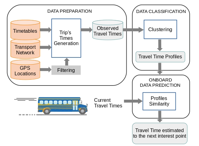
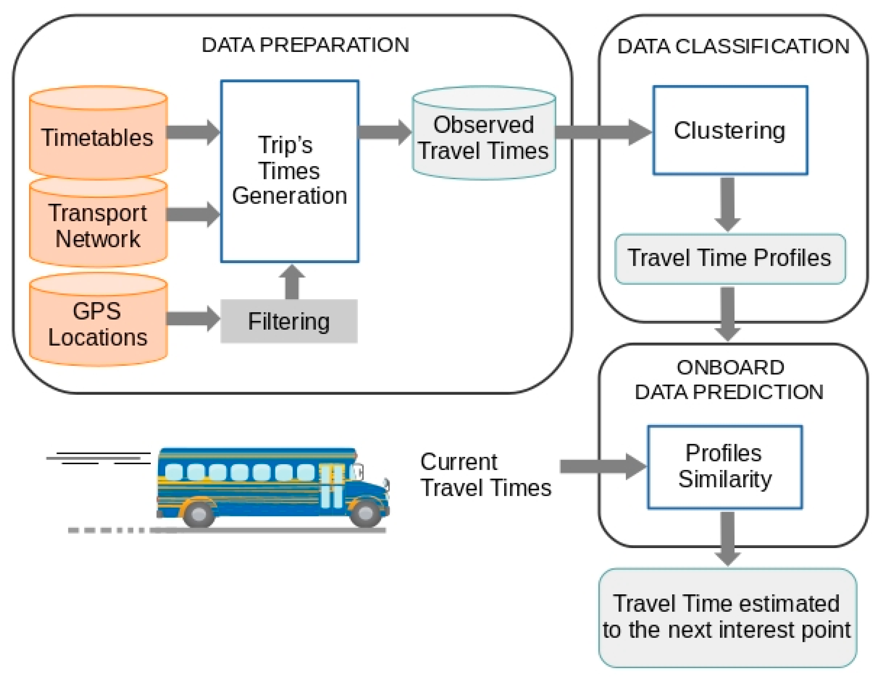
As discussed in the previous section, in the context of regular road passenger transport, the short-term TT prediction methods take into account historical TT behaviour, modelled using different techniques such as ANN, SVM, STS, etc., and current behaviour, usually represented by the time taken by the vehicle to travel the last segment it has completed. The proposed method is based on the idea that it is possible to predict short-term TT using the representative elements from a classification process to represent historical behaviour, and the TT observed at all points of interest through which the vehicle has already passed to represent current TT behaviour (see Figure 1). Considering these working principles, the proposed prediction method has some interesting properties in relation to the techniques described in the review of the previous section. These properties are:
- Historical TT behaviour models that use patterns obtained through clustering techniques are much less costly, from the computational point of view, than the techniques usually used for this purpose, such as ANN, SVM and STS.
- The historical TT behaviour model can be applied to all routes on a transport network more easily than when using the alternative techniques mentioned above. In a TT prediction scenario for all the routes on a public transport network, representing historical TT behaviour by means of clustering techniques would first require the appropriate number of classes to be determined for each route. This could be done systematically using metrics that measure the quality of the resulting clusters. However, the use, for example, of ANN or SVM, to model TT behaviour on all the routes would require different configurations that would have to be obtained through learning and validation processes.
- A third advantage, resulting from the two previous advantages, is that the continuous evolution of the representation of historical behaviour by means of clustering techniques is less costly than with the alternative techniques mentioned above. This continuous evolution is necessary because TT depends on external factors that are variable over time.
For the representative elements obtained through a clustering process to reflect historical TT behaviour, a significant sample of TT is needed. As explained in the review of the previous section, there are mainly two data sources from which to obtain a sample of historical TT values: AVL and APC. Although the proposed method is independent of the data source that is used to obtain the historical TT data records, in the use case presented in the fourth Section AVL systems are used as the data source. In this implementation, the basic data are the GPS locations of the vehicle. In order to carry out this analysis of the routes, it is also necessary to handle data of a different nature, which are typically used in public transport operations (transport network design and operations control).
3.1. Formal Model Framework
The objective of the proposed method is to estimate short-term TT in a context of regular passenger road transport planned by timetable. As already mentioned above, this type of TT prediction is executed and is valid during the trip made by a public transport bus as it operates a particular route. In this section, entities related to the proposed method are presented and formalised. Table 2 includes the notation used for the model entities.
3.1.1. Definition of the Entities Used by the Model
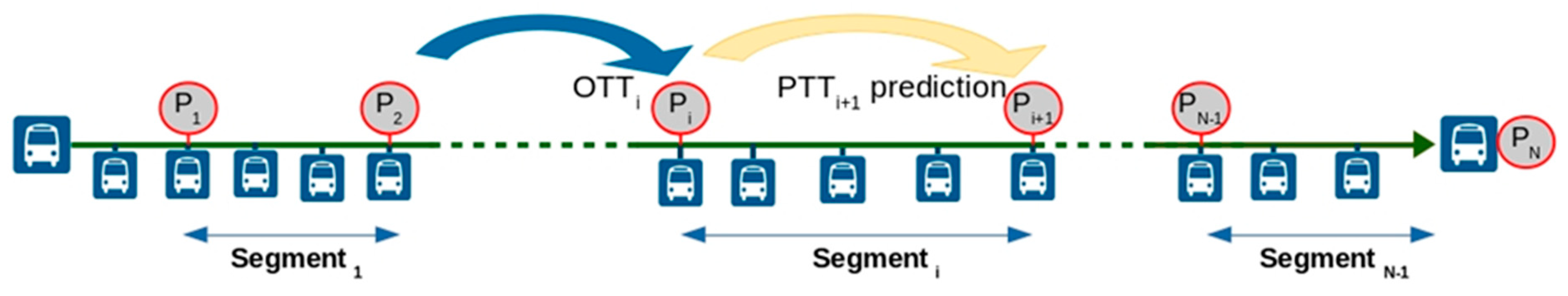
The first entity to be formalised is the public transport line. For the purposes of this paper, a line is defined as systematic, scheduled route taken by public transport buses. Systematic means that the bus always follows the same route and stops at a series of pre-established stops that do not vary. Scheduled means that there is a schedule that establishes when the buses must run the route. The operation of a line by a public transport vehicle shall be termed a trip. In the model, L represents a generic line and a specific line is specified by means of the notation Lc, where the subscript c is an integer value that uniquely identifies the line. Trips on Lc are specified by means of the notation Ec, where c is the identifier of the line. In the model, time is specified by the notations T and t. T represents a time interval and t represents a moment of time, which is the minimum unit of time. All trips by line Lc that have been made over a period of time T are specified by the notation Ec,T. Similarly, a trip that has begun at a moment of time t is specified by means of the notation ec,t. Stops on the route of Lc are represented by the notation Sc. In the context of this study, stops on a route for which the TT is to be predicted are called points of interest and are represented by Pc. Points of interest on the route of Lc are designated by the notation Pc,i, where the subscript i identifies the point of interest and its value matches the order in which the bus passes them following the planned route. For example, Pc,1 is the first point of interest through which the vehicles pass when operating route c. When selecting points of interest, the only restriction is that the first stop of the route cannot be a point of interest. The section of the route that runs from one point of interest to the next is called a route segment (see Figure 2). In this figure, the blue rectangles represent the stops and the red circles, the points of interest.
In the context of regular passenger road transport, TT is the result of the sum of two times: dwell time, DT, and nonstop running time, RT. DT represents the time that the vehicle is stationary at stops for passengers to board or alight from the vehicle. RT represents the time taken by the vehicle to go from one stop on the route to the next. If a route has N stops, then the total TT of a trip is:
The term arrival time is the time at which the vehicle arrives at that stop. The arrival times observed at the points of interest on trip ec,t are represented by OPTc,t. If Lc has N points of interest, then the arrival times of each entity OPTc,t are recorded as an array of N integer values. The set comprising the arrival times on all trips on a route completed by Lc in a time period T is represented by OPTc,T. The prediction made by the proposed model consists of estimating the time that elapses between the vehicle reaching point of interest i and point of interest i + 1. Therefore, the DT at point of interest i is included in this time.
3.1.2. The k-Medoid Clustering Technique
Clustering methods are classification techniques that group large sets of elements, characterised by a set of attributes, using similarity criteria. For the purposes of this study, clustering techniques have two interesting properties. The first is that they do not require prior learning and the second is that there are metrics that measure the quality of the resulting clusters. In the proposed model, assuming the formulation stated above, given a significant period of time T and a route Lc, the set of elements to be classified is composed by all the trips on route Lc that have been completed in period T—i.e., dataset Ec,T representing all trips ec,t. These trips are represented by the TT observed at each point of interest OPTc,t and the dataset of all the representations of all trips Ec,T is represented by OPTc,T. If in the prediction of TT, n points of interest have been defined on Lc, then each element OPTc,t, is represented by an n-tuple (TT1, TT2, …, TTn), which corresponds to the TT observed on trip ec,t.
In the proposed methodology, the historical TT behaviour profiles are obtained by the k-medoids method [20]. This method belongs to the group of non-hierarchical clustering techniques, and any distance metric can be used to measure the similarity between two elements. The grouping criterion is to cluster data around the most representative objects, called the “medoid”, of the dataset. The most representative object is the most centrally located point. Therefore, this representative object is a pre-existing object from the sample and not an object that is generated in the classification process. This property means that the k-medoids technique responds well in the event of outliers. The most used distance metrics in the k-medoids technique are the Euclidean distance and Manhattan distance metrics. Equations (2) and (3) express the Euclidean and Manhattan distances, between two objects, Xi and Xj, for a set of Q objects, each object being represented by n attributes. Equation (2) is the Euclidean distance and Equation (3) the Manhattan distance.
An example of clustering using the k-medoids technique is shown in Figure 3. On the horizontal axis the points of interest are represented and on the vertical axis the observed TT, measured in seconds, at the points of interest of a route. Each grey curve represents the TT recorded for a trip, OPTc,t. The dataset OPTc,T is formed by all the OPTc,t curves. The red, blue and green curves represent the medoids, which are the representative object of each of the three resulting clusters.
To evaluate the validity of a clustering solution there are different criteria, which may be classified into three categories: external indices, which measure the extent to which cluster labels match externally-supplied class labels; internal indices, which measure the intrinsic information of each dataset; and relative indices, which are used to compare several different clustering solutions. For the purposes of this study, an internal index was chosen to measure the quality of the clusters: the silhouette function [21]. This measures the consistency of the cluster based on a comparison of the tightness and separation of the elements of each segment generated. This is computed by the following expression:
In expression (4), Ai is the average distance from object i to the other objects within the cluster and Bi is the smallest average distance from i to all the objects of each of the clusters to which i does not belong. The values returned by the silhouette function are in the range −1 and 1. A value close to 1 indicates a high degree of consistency in the resulting clusters and, conversely, a value close to −1 indicates that the resulting clusters have little consistency.
3.2. Travel Time Prediction Scheme
Taking the concept of point of interest, if we assume that a vehicle is at point Pi of the sequence of points of interest on route Lc, the objective of the proposed method is to estimate the TT required to reach the next point in the sequence of points of interest of the route, i.e., the TT to reach point Pi+1. The recent history for that vehicle, located at point of interest Pi, is represented by a set of ordered values that represent the TT observed when going through the points of interest already travelled, represented by the i-tuple (TT1, TT2, …, TTi). Past history, in period T, is represented by the medoids resulting from applying the k-medoid clustering technique to the set OPTc,T, these medoids represent the historical profiles of the TT. When the vehicle is at Pi, the TT to reach point Pi+1 is estimated in two steps. In the first step, from the observed TT (TT1, TT2, …, TTi) the medoid that has the most similar behaviour to the TT behaviour recorded up to point Pi is selected. The similarity metric used is the same as that used in the clustering process through which the medoids were obtained. Once the most similar medoid has been selected, then the prediction of the TT for segment Si, i.e., to reach point Pi+1, is:
In Equation (5), PTTi+1 represents the prediction of the TT taken to reach point Pi+1. TTi is the TT observed at point Pi and Mk is the medoid to which the recorded TT are most similar. Mk,i and Mk,i+1 represent the attributes i and i + 1 of this medoid, i.e., the TT that represent the historical behaviours at points Pi and Pj+1 of the k cluster.
Next, the short-term TT prediction algorithm is described for trip ec,t that is completed in vehicle V.
Data:
- K: number of clusters used to represent historical TT behaviour;
- {M1, …, Mk}: set of k-medoids that represent TT behaviour on trips on route Lc;
- i: last control point through which V has passed on trip ec,t;
- TT1→i: observed arrival time at interest points 1, 2, …, i on trip ec,t (recent behaviour);
- Mk,1→i: for the k-medoid, values of the arrival time at interest points 1, 2, …, i (historical behaviour);
- PTTi+1: objective of the algorithm, which is to predict TT at interest point i + 1.
Step 1. Obtain the medoid that most resembles the observed TT behaviour up to the last interest point that V has passed on trip ec,t. Dist(a,b) is the function that evaluates the distance metric that is used to assess similarity.
Dmin = ∞
For (j = 1 to K) do
Do
D = Dist(Mk,1→i, TTi→1)
If (D < Dmin)
Begin
k = j
Dmin = D
End
End
Step 2. Estimate PTTi+1
PTTi+1 = TTi + Mk,i+1 − Mk,i
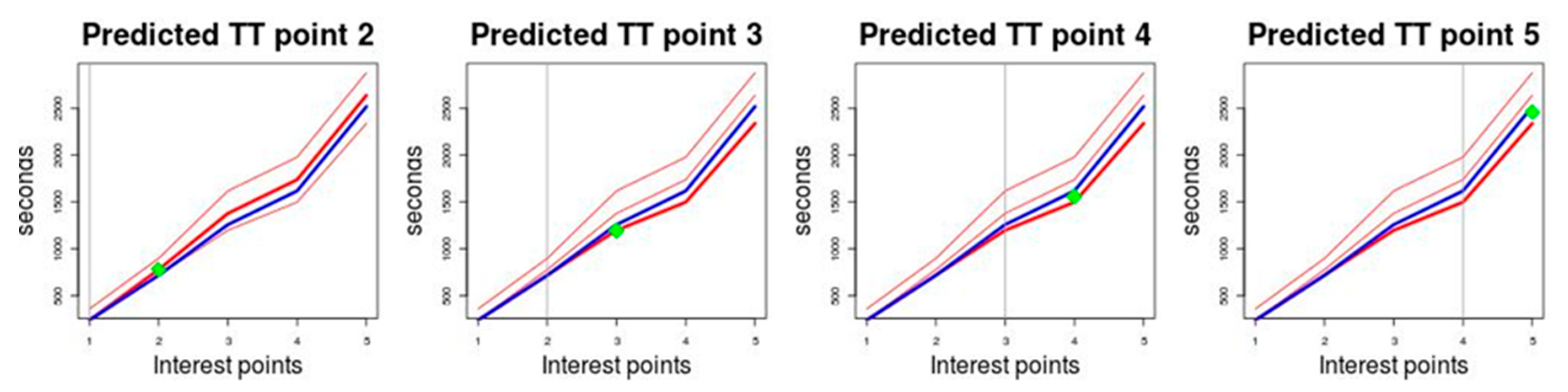
The prediction method is illustrated graphically in Figure 4. This illustrates the prediction for a route on which five points of interest have been defined and that are represented on the horizontal axis. The TT measured in seconds is represented on the vertical axis. The historical behaviour is represented by three medoids that have been drawn in red. The blue graph represents the TT of the test trip for which the prediction is being made and the green dot is the TT value predicted for the different points of interest. Table 3 illustrates the prediction method numerically with an example prediction of a trip. The route in this example has five points of interest, columns P1, P2, P3, P4 and P5. The historical TT behaviour is represented by three medoids, rows M1, M2 and M3. The observed TT up to each of the points of interest is displayed in row TT. As the vehicle reaches each point of interest, the medoid with the behaviour that is most similar to the TT observed on the trip is selected, using Manhattan distance as the similarity metric. Rows D(TT,M1), D(TT,M2) and D(TT,M3) contain the values resulting from calculating this distance between TT and M1, M2 y M3, respectively. At point of interest P1, we calculated the distance between the TT observed at this point, which was 180, and the values of the medoids at this point, which were 360 for M1, 240 for M2 and 240 for M3. The Manhattan distance values obtained were 180 for D(TT,M1), 60 for D(TT,M2) and 60 for D(TT,M3). Since the minimum distance value obtained was 60 and it was obtained with two medoids, M2 and M3, the first medoid that produced this minimum value, in this case M2, was selected for this method. The predicted TT values at each point Pi are displayed in row PTT. The TT prediction to reach point of interest P2 will be made taking medoid M2 as the historical reference and the prediction will be calculated, according to Equation (5), by adding to the TT observed at P1, which is 180 s, the difference between the TT value of M2 at point P2, which is 780 s, and the value of M2 at point P1, which is 240 s. Therefore, the value of the TT prediction to reach P2 is 720 s. The TT prediction to reach point P3 would be carried out analogously to this, but in this case the TT profile on the trip will consist of two values (180,720) and the historical TT behaviour profiles will be (360,900) according to M1, (240,780) according to M2 and (240,720) according to M3. At this point the historical profile that is most similar to the profile observed on the trip is that represented by medoid M3. As shown in Table 3, at the rest of the points of interest, M3 is the medoid with a profile most similar to the observed TT values and therefore its TT values will be those used to make the predictions at the other points.
4. Results and Discussion
The main objectives of the tests were to select the most suitable parameters for the proposed method, to evaluate its prediction accuracy and to compare it with other methods. To make this analysis more complete, data were collected from two bus lines with different characteristics in terms of demand, route length, types of road and the population centres that they run through.
In terms of resources and tools, a computer with an Intel(R) Core (TM) i7-2600K CPU processor @ 3.40GHz with 16 GB RAM was used. Oracle DB—the database environment used by the transport operator that provided its data—was used to prepare the data. For the modelling phase, the RStudio framework was used, specifically Cluster Package [22] and Neuralnet Package [23]. To visually map the data, the GoogleMap framework was used.
4.1. Description of Datasets
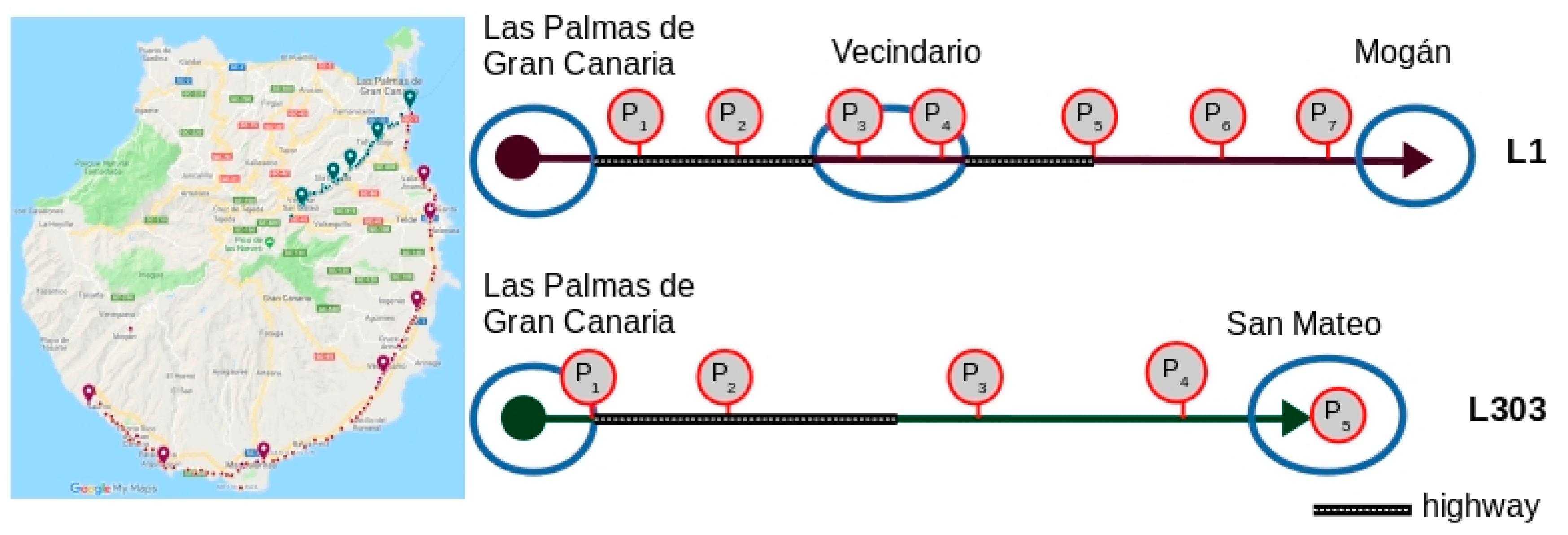
The datasets used came from the operational records of two lines operated by the intercity public transport network of the Island of Gran Canaria. The period of time analysed in the study was the whole of 2015. Therefore, according to the model, the value of T is the year 2015. These two lines, identified by codes L1 and L303, cover two important transport corridors on the Island. Line L1 covers the Capital-South corridor, starting in the city of Las Palmas de Gran Canaria, which, as the most populated urban nucleus where the main public service centres of the island are based, is the main transport generation point. The line goes through the main tourist centres—tourism is the largest sector of the island economy and generates the most employment. Line L303 covers the Capital-Centre corridor, starting in the city of Las Palmas de Gran Canaria and travelling through the largest population centres in the centre of the island. Table 4 shows the length and number of stops on these routes, and the number of stops selected for the study—the points of interest. In the case of line L1, of the 91 stops, 7 points of interest were selected. In the case of line L303, six were selected, giving rise to five route segments. Two aspects were taken into account when selecting stops as points of interest: the number of travellers and the distance between the stops (stops very close to each other were ruled out). The routes taken by the two lines travel along different types of road (fast roads, rural roads and urban roads) and, due to the different motivations and type of user, moments of peak and off-peak demand vary. Figure 5 shows the routes of these lines. On the left side of the figure, the route is shown on a map of the island, where the dots marked on each route represent the stops, and the balloon markers the points of interest selected for the study. On the right side, a schematic representation of the routes is displayed.
The basic data unit used was the GPS location data that each bus automatically records every minute. In order to obtain all the TT for the trips completed in 2015, a data mining process was carried out to reconstruct all the trips on the routes to be analysed. Table 5 shows the number of location records used to reconstruct the route trips (NGPS), the number of reconstructed trips (NRE) and the number of these trips for which the routes are consistent with the planned route and do not have errors (NCRE). The set of correct trips is dataset E1,2015 in the case of L1, and E303,2015 for L303.
4.2. Performance of the Method Using Different Configuration Parameters
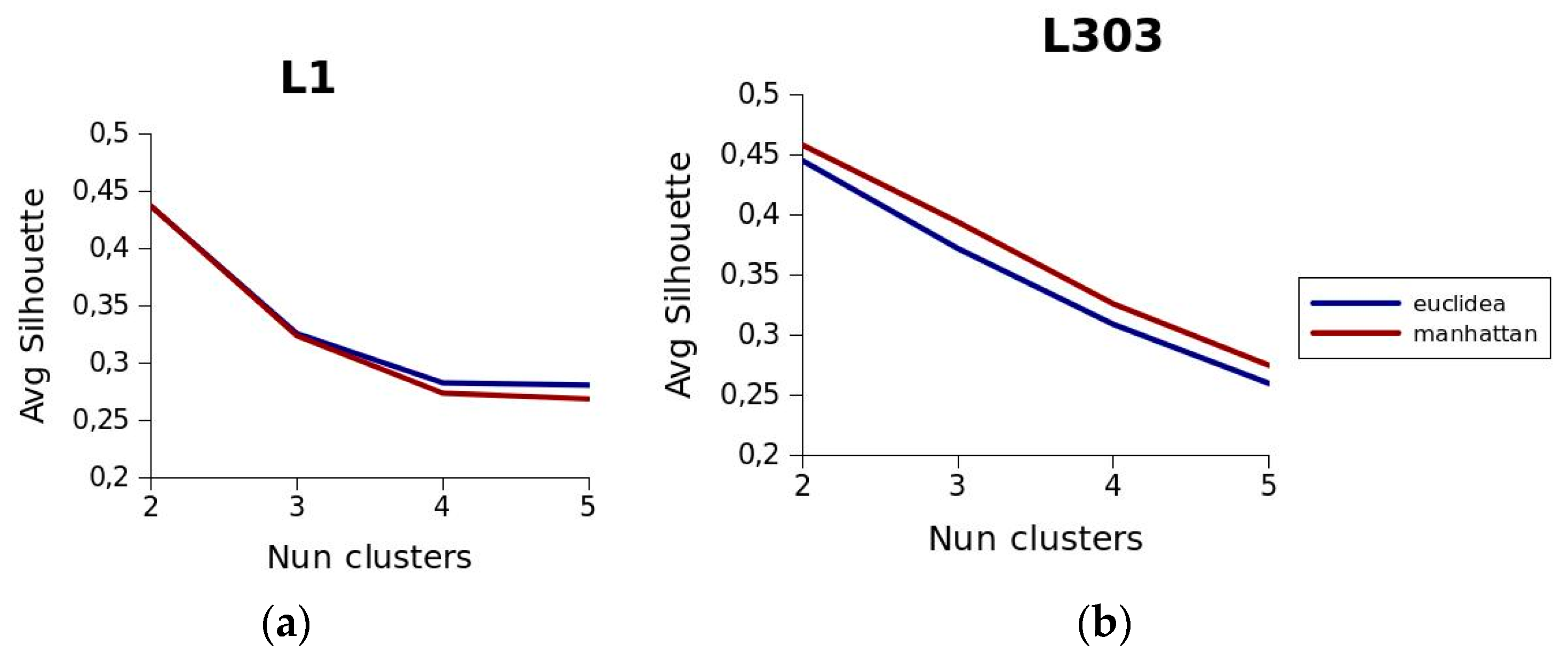
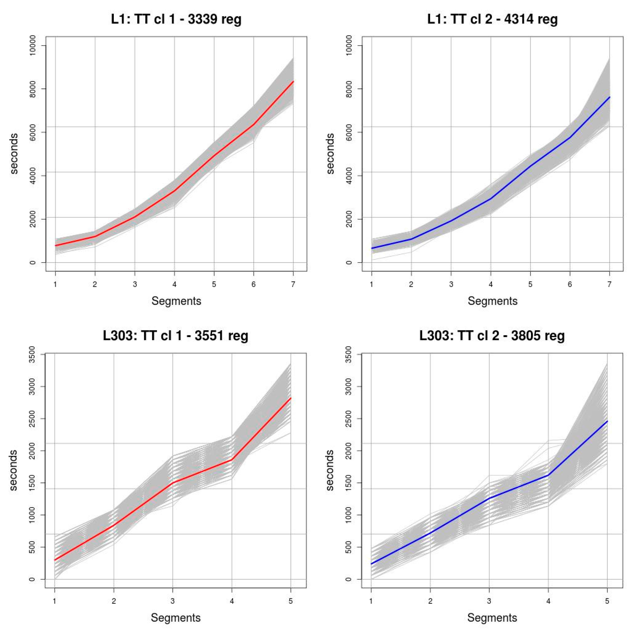
The first phase of the tests was designed to check how the distance metric and the number of clusters affected the process of creating the clusters. Two distance metrics were tested: the Euclidean and the Manhattan. These metrics were used to generate different segments in the OPT1,2015 and OPT303,2015 datasets, specifying different numbers of clusters beforehand, and evaluating the quality of the resulting segments with the silhouette function. Figure 6 shows the values returned by the silhouette function. The number of clusters used is represented on the horizontal axis and the resulting value of the function on the vertical axis. Based on the results obtained, we decided to use the Manhattan distance as the distance metric and to partition the data into two clusters. As can be seen, the behaviour of this function is very similar in the case of route L1. However, it may be observed in the case of route L303 that the function produces higher values, that is, higher levels of consistency in the clusters, when the Manhattan distance is used. Regarding the number of clusters, the best levels of consistency, regardless of the route analysed and the metric used, occur when two clusters are used. Indeed, both for route L1 and for route L303, the values of the silhouette function are very close to 0.45 using both the Euclidean metric and the Manhattan metric. It may also be observed that, irrespective of the route analysed and the distance metric used, as we increase the number of clusters used in the clustering process, the value of the silhouette function decreases, which means that the degree of consistency decreases. Figure 7 shows the result of grouping routes L1 and L303 using two clusters. The objects of the clusters are drawn in grey and the medoids of each cluster are drawn in red and blue. These medoids are the ones used in TT predictions that are displayed as results.
4.3. Evaluation of Prediction Accuracy
The metric used to evaluate prediction accuracy for a trip was the mean absolute percentage error (MAPE), which is expressed according to Equation (6). In this equation, N represents the number of points of interest on the route, i varies between 1 and the total number of segments. OPTi is the TT recorded for segment i and PTTi is the predicted TT for segment i. Both OPTi and PTTi are expressed in seconds. For this evaluation, all OPT1,2015 and OPT303,2015 data records were used for the samples.
Table 6 shows the results obtained for the trips completed by each bus line. The AVMAPE row represents the average value for all the trips, and the Si rows show the average MAPE value for each segment of the route. With regard to L1, the worst prediction was made for segment S1, since this is where the highest MAPE value (0.1549) was obtained: on this segment the percentage of error in TT prediction in relation to the observed value was 15.49%. The best prediction was made for segment S4, where an error percentage of 7.61% was obtained. The average value, considering the MAPE values for all segments of the route—AVMAPE row—was 0.1106. Therefore, considering the MAPE values for all the segments, PSM commits an error of, on average, 11.06% of the observed TT values. With regard to L303, S2 was the segment for which the highest MAPE value (0.223) was obtained: on this segment the percentage of error in the prediction, in relation to the observed value, was 22.49%. The best prediction was made for S4, where the lowest MAPE value (0.0939) was obtained: an error percentage of 9.39% in relation to the observed TT values on that segment. The average value, considering the MAPE values for all segments of the route—AVMAPE row—was 0.1325, i.e., the average error rate was 13.25% in relation to the TT observed for all segments.
4.4. Comparison with Other Prediction Methods
PSM was compared with two reference methods that are widely used in the proposals described in the section on short-term TT prediction methods. These alternative methods are: predictions based on the average TT obtained from the observed TT (AvgTT) and an ANN prediction model. The analysis consisted of comparing the MAPE values obtained from these alternative methods with the values provided by the proposed method. The resulting MAPE values were compared on each segment of the analysed routes as well as the global value obtained for all the routes. The required processing times of each method were also compared.
The ANN model used for the comparison was the MLP network, analogous to that used in [6]. The input variables for the network were time of day, the identification of the point of interest i that the vehicle has arrived at, and the TT observed since the beginning of the route. The output variable of the network was the TT of the vehicle in segment i. The dataset used for training the two ANNs, one for each route, was built with 80% of the data records from the OPT1,2015 and OPT303,2015 datasets and the test dataset used the remaining 20%. Based on the results of the tests, using three, four and five nodes in the hidden layer, the configuration with three nodes was chosen as the configuration with the best results.
4.4.1. Comparison of Prediction Accuracy
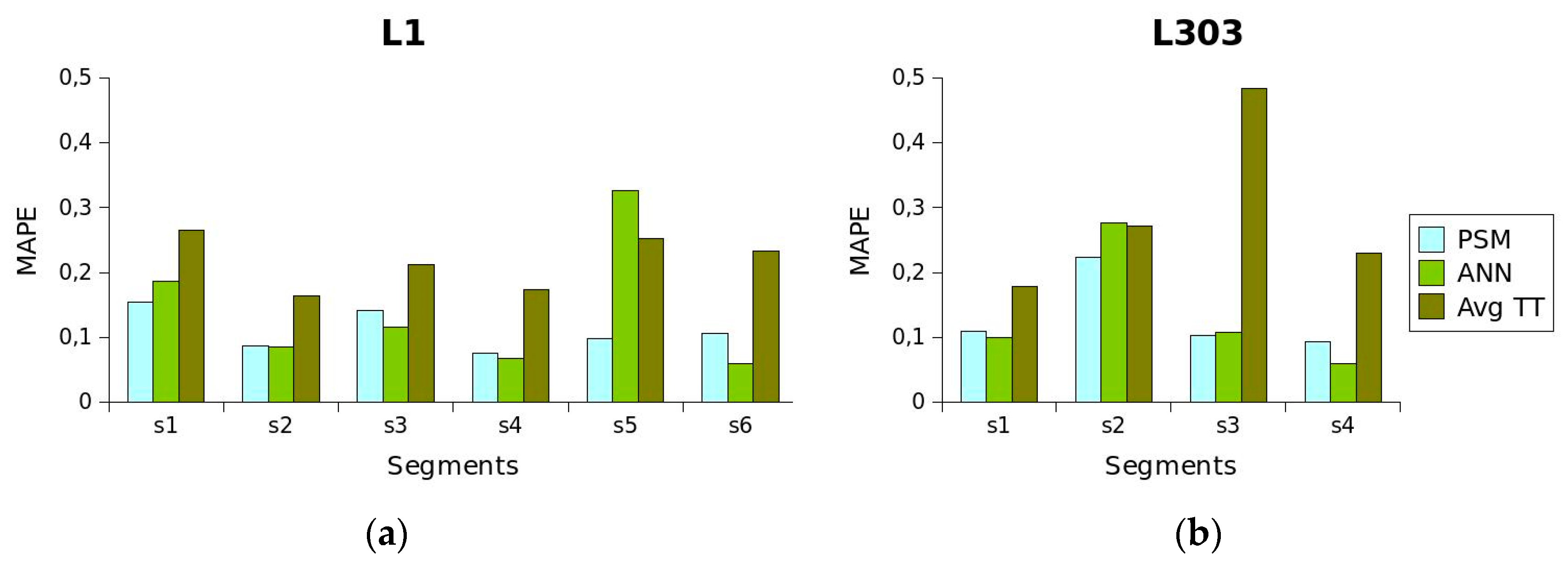
Figure 8 shows the results obtained by applying each of these methods to the two routes analysed. As shown in Figure 8a, the results obtained for route L1 clearly indicate that AvgTT produces the worst results. PSM provided better results for S1 and S5 compared to the ANN and AvgTT methods, obtaining a considerably better prediction for S5 segment. ANN produced better results for S3 and S6. On S2, the MAPE values obtained by the PSM and ANN methods were practically the same. If the MAPE values obtained for all the segments are taken into account, the conclusion drawn is that PSM produces values that vary less than those produced by AvgTT and ANN. PSM performed the worst on S1, with an MAPE value close to 0.15. The best PSM performance was obtained on S4, with a value close to 0.07. In the case of ANN, it performed best on S6, with a value close to 0.06, and worst on S5, with a value close to 0.32, which even exceeded the value obtained for that segment by AvgTT. The results obtained for route L303 are shown in Figure 8b. These results also clearly indicate that AvgTT provides the worst results. PSM produced better results than AvgTT and ANN on segments S2 and S3. ANN produced better results on segments S1 and S4. As was the case with line L1, if the MAPE values obtained for all the sections are taken into account, PSM produces values that vary less than those produced by AvgTT and ANN. It can be seen that the worst performance of PSM was on segment S2, with a MAPE value close to 0.22. For the rest of the segments, the values obtained were similar and close to 0.10. In the case of ANN, the best performance was on segment S4, with a value close to 0.05, and the worst on S2, with a value close to 0.27, very close to the value obtained for that segment by AvgTT.
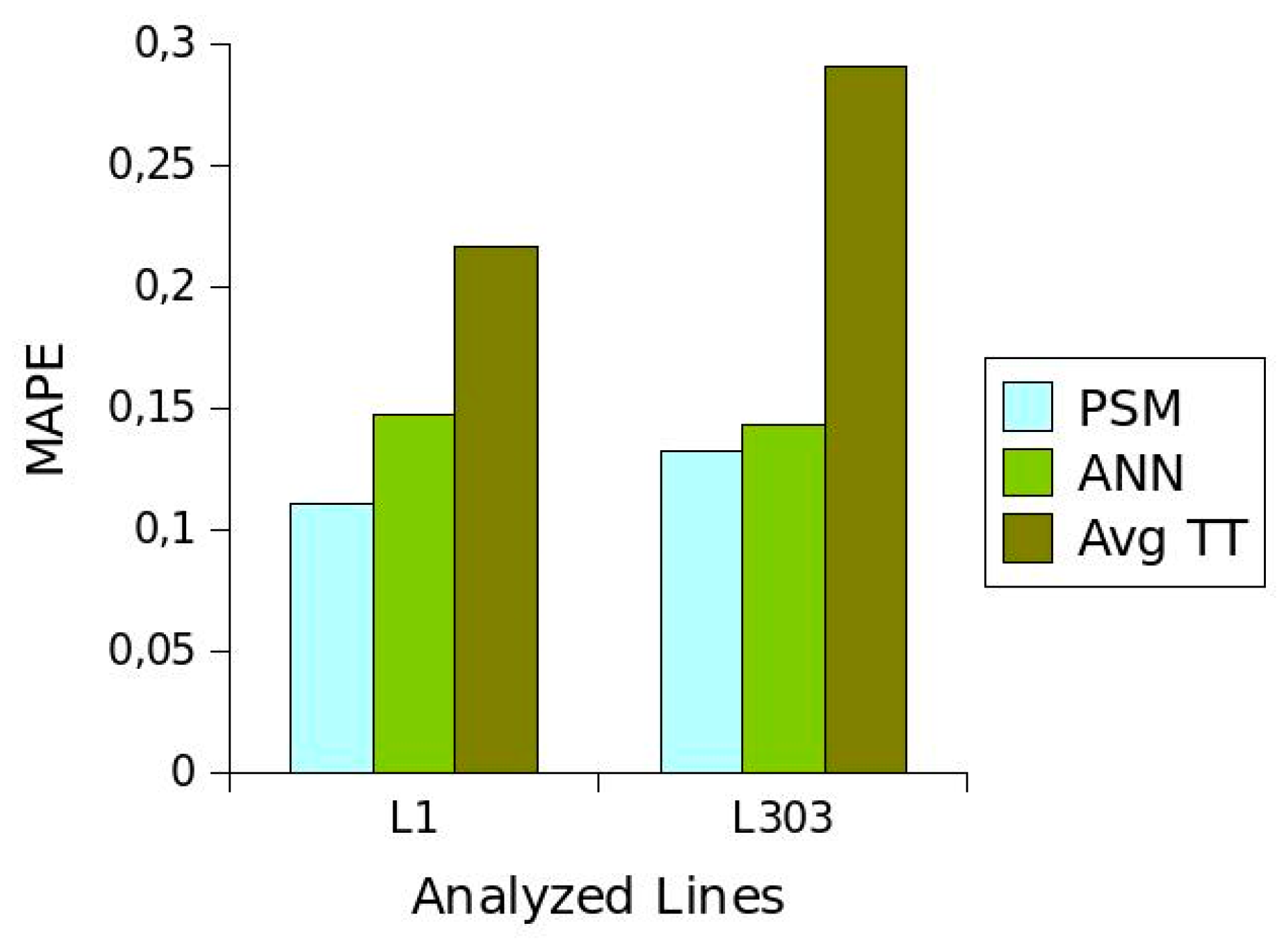
Figure 9 shows the average MAPE values obtained for each segment of each of the routes analysed. It can be seen that PSM performed the best since it provided a value close to 0.11 on L1 and 0.13 on L303. In the case of ANN, the average MAPE values obtained for the two routes were similar, and close to 0.14. The worst-performing method was clearly AvgTT with values of 0.21 and 0.29 for L1 and L303, respectively.
4.4.2. Comparison of Complexity of the Required Processes and Computation Time
Although substantial differences were not observed between the results obtained by PSM and ANN in all cases, certain aspects that make PSM more attractive need mentioning. First, it is not necessary to normalise the data, as is the case of ANN where this needs to be done to. On the one hand, avoid differences between the magnitudes of the variables that affect the calculation of the weightings during the training phase. On the other hand, adapt them to the corresponding ranges of the different activation functions. Second, there are considerable differences between the time used to create the TT profiles used by PSM, and the time spent on the ANN training process. For example, on one of the analysed routes the training of the network took 59 times longer than the clustering process, as can be seen in Table 7, where the times spent on each case are shown. Third, while it is possible to find evaluation functions for the generated clusters, the number of nodes of the hidden layer has to be determined in the experimental phase, so it is easier to find an optimal configuration in the PSM model. Fourth and lastly, ANN errors have greater variability, as can be seen especially in the case of line L1 (Figure 8a).
4.5. Final Discussion
Considering the results, it can be said that PSM provides a prediction accuracy similar to that provided by ANN. However, PSM is more stable behaviour in the accuracy of its predictions. In addition, the behaviour patterns represented by the medoids used in PSM provide interpretable information about TT, an advantage that ANN and other models with high predictive power—described in Table 1, such as proposals based on SVM—do not have. Considering another property shown in Table 1—the ease of applying the method to all the routes on a transport network—PSM is easier to apply, with lower computational cost, than models based on ANN. In this regard, the computational cost of applying PSM to TT predictions on all routes of a transport network is considerably lower than that of applying techniques based on ANN. This is because PSM does not require training processes for its application, whereas ANN-based prediction systems do require learning, which would also have to be done for each route of the transport network. Given the characteristics of the SVM-based methods—another method with high predictive power—PSM would also be easier to apply to all the routes of a transport network, with a lower computational cost.
As with the ANN-based methods, the predictions made by PSM in situations involving exceptional conditions, such as for example abnormally slow speed of the vehicle due to traffic incidents, have a lower accuracy. For this reason, the combined prediction methods ANN-KFM or SVM-KF were used. Therefore, it may be inferred that the use of a combined PSM-KF model could be used in contexts in which recent historical information provided by other vehicles was available, as in the case of urban transport. Finally, we would like to underscore the fact that the low computational cost of making TT predictions with PSM would enable predictions to be calculated on the vehicle itself.
5. Conclusions
In this article, a short-term TT prediction model for public transport buses is proposed. To estimate TT, the model takes into account the historical behaviour of TT, represented by the medoids resulting from a clustering process based on the k-medoids technique, and the current TT behaviour, which is represented by the TT observed on the vehicle for which the prediction is made. Therefore, the method does not require recent TT data provided by other vehicles, meaning that it can be executed autonomously on the vehicles themselves. The method has been applied in two real cases of public transport lines of different characteristics. The results show that, in general, the average error made in the predictions is around 13% of the observed TT values, a result similar to that obtained by the alternative method ANN, although its variability is less than this alternative method. The proposed method has some interesting features. The first is that, since it does not need recent TT data provided by other vehicles, the method can be used in the context of line services planned by timetable, which is the planning method used for intercity transport. Second, the method not only provides short-term TT estimates; by using the k-medoids clustering technique to extract TT patterns from bus trips, it also provides information on its behaviour, thus helping to make long-term TT predictions, which are used in the planning of line services. Both from the computational point of view and the configuration of the required parameters, the method is less costly than the most widely used alternative methods, based on machine learning regression or state-based time-series, because it does not require costly learning processes and validation. Therefore, the prediction of short-term TT on all the routes of a transport network can be carried out by the proposed method at considerably lower cost.
Author Contributions
The analysis of the transport data and the design of the data mining processes to obtain the basic data used in this study were done by T.C., G.P. and C.R.G.; all the authors of this article participated in the conceptualisation and formulation of the proposed model; T.C., G.P. and F.A. participated in the tests carried out with clustering techniques; T.C., A.Q.-A. and G.d.B. participated in the tests performed with ANN; the research work was coordinated by C.R.G. All the authors participated in the writing of this manuscript.
Funding
This research received no external funding.
Acknowledgments
The authors wish to express their gratitude to the public transport company Global Salcai-Utinsa S.A for allowing access to its transport database.
Conflicts of Interest
The authors declare no conflict of interest.
References
- EN13816. Available online: https://ec.europa.eu/eip/ageing/standards/city/transportation/en-138162002_en (accessed on 3 March 2019).
- Peek, G.J.; van Hagen, M. Creating synergy in and around stations: Three strategies for adding value. Transp. Res. Rec. 2002, 1793, 1–6. [Google Scholar] [CrossRef]
- Yetiskul, E.; Senbil, M. Public bus transit travel-time variability in Ankara (Turkey). Transp. Policy 2012, 23, 50–59. [Google Scholar] [CrossRef]
- Comi, A.; Nuzzolo, A.; Brinchi, S.; Verghini, R. Bus travel time variability: Some experimental evidences. Transp. Res. Procedia 2017, 27, 101–108. [Google Scholar] [CrossRef]
- Yu, B.; Yang, Z.; Yao, B. Bus Arrival Time Prediction Using Support Vector Machines. J. Intell. Transp. Syst. 2007, 10, 151–158. [Google Scholar] [CrossRef]
- Chang, H.; Park, D.; Lee, S.; Lee, H.; Baek, S. Dynamic multi-interval bus travel time prediction using bus transit data. Transportmetrica 2010, 6, 19–38. [Google Scholar] [CrossRef]
- Lee, W.-C.; Si, W.; Chen, L.-J.; Chen, M.C. HTTP: A New Framework for Bus Travel Time Prediction Based on Historical Trajectories. In Proceedings of the International Conference on Advances in Geographic Information Systems (ACM SIGSPATIAL GIS 2012), California, CA, USA, 6–9 November 2012. [Google Scholar] [CrossRef]
- Gurmu, Z.K.; Nall, T.; Fan, W. Artificial Neural Network Travel Time Prediction Model for Buses Using Only GPS Data. J. Public Transp. 2007, 17, 45–65. [Google Scholar] [CrossRef]
- Gal, A.; Mandelbaum, A.; Schnitzler, F.; Senderovich, A.; Weidlich, M. Traveling time prediction in scheduled transportation with journey segments. Inf. Syst. 2017, 64, 266–280. [Google Scholar] [CrossRef]
- Arhin, S.; Stinson, R.Z. Transit Bus Travel Time Prediction using AVL Data. Int. J. Eng. Res. Technol. 2016, 5, 21–26. [Google Scholar] [CrossRef]
- Zhang, J.; Wang, F.; Wang, S. Application of Support Vector Machine in Bus Travel Time Prediction. International. J. Syst. Eng. 2018, 2, 21–25. [Google Scholar] [CrossRef]
- Shalaby, A.; Farhan, A. Prediction Model of Bus Arrival and Departure Times Using AVL and APC Data. J. Public Transp. 2004, 7, 41–61. [Google Scholar] [CrossRef] [Green Version]
- Vanajakshi, L.; Subramanian, S.C.; Sivanandan, R. Travel time prediction under heterogeneous traffic conditions using global positioning system data from buses. IET Intell. Transp. Syst. 2008, 3, 1–9. [Google Scholar] [CrossRef]
- Song, X.; Teng, J.; Chen, G.; Shu, Q. Predicting bus real-time travel time basing on both GPS and RFID data. In Proceedings of the 13th COTA International Conference of Transportation Professionals (CICTP 2013), Shenzhen, China, 13–16 August 2013. [Google Scholar] [CrossRef]
- Chen, M.; Liu, X.; Xia, J.; Chien, S.I. A Dynamic Bus-Arrival Time Prediction Model Based on APC Data. Comput. Aided Civ. Infrastruct. Eng. 2004, 19, 364–376. [Google Scholar] [CrossRef]
- Bai, C.; Peng, Z.-R.; Lu, Q.-C.; Sun, J. Dynamic Bus Travel Time Prediction Models on Road with Multiple Bus Routes. Comput. Intell. Neurosci. 2015, 2015, 1–9. [Google Scholar] [CrossRef] [PubMed] [Green Version]
- Fan, W.; Gurmu, Z. Dinamic Travel Time Prediction Models for Buses Using Only GPS Data. Int. J. Transp. Sci. Technol. 2015, 4, 353–366. [Google Scholar] [CrossRef]
- Jairam, R.; Kumar, B.A.; Arkatkar, S.S.; Vanajakshi, L. Performance Comparison of Bus Travel Time Prediction Models across Indian Cities. Transp. Res. Rec. 2018, 2672, 87–98. [Google Scholar] [CrossRef]
- Hua, X.; Wang, W.; Wang, Y.; Ren, M. Bus arrival time prediction using mixed multi-route arrival time data at previous stop. Transport 2018, 33, 543–554. [Google Scholar] [CrossRef]
- Kaufman, L.; Rousseeuw, P.J. Partitioning around Medoids (Program PAM). In Finding Groups in Data Finding Groups in Data: An Introduction to Cluster Analysis; Kaufman, L., Rousseeuw, P.J., Eds.; Wiley: Hoboken, NJ, USA, 2009; pp. 68–125. [Google Scholar] [CrossRef]
- Rousseeuw, P.J. Silhouettes: A graphical Aid to the Interpretation and validation of Cluster Analysis. J. Comput. Appl. Math. 1987, 20, 53–65. [Google Scholar] [CrossRef]
- Cluster Analysis Basics and Extensions. R Package Version 2.0.6. Available online: https://CRAN.R-project.org/package=cluster (accessed on 21 March 2019).
- Neuralnet: Training of Neural Networks. R Package Version 1.33. Available online: https://CRAN.R-project.org/package=neuralnet (accessed on 13 December 2017).
Figure 1.
Overview of the TT prediction model.

Figure 2.
Schematic representation of a route according to the model.

Figure 3.
Representation of trip data and resulting medoids.

Figure 4.
Schematic representation of the prediction method.

Figure 5.
Representation of the two lines analysed.

Figure 6.
Behaviour of the silhouette function for each route depending on the number of clusters used in the clustering process. (a) Route L1; (b) Route L303.
Figure 6.
Behaviour of the silhouette function for each route depending on the number of clusters used in the clustering process. (a) Route L1; (b) Route L303.

Figure 7.
Clusters resulting from applying the k-medoids technique with two clusters to the TT observed on the trips.
Figure 7.
Clusters resulting from applying the k-medoids technique with two clusters to the TT observed on the trips.

Figure 8.
MAPE values obtained by applying the three methods. (a) Values obtained for L1. (b) Values obtained for L303.
Figure 8.
MAPE values obtained by applying the three methods. (a) Values obtained for L1. (b) Values obtained for L303.

Figure 9.
Average MAPE values for each method on each of the lines studied.


Table 1.
Advantages and disadvantages of short-term TT prediction models.
| Model | Technique | Advantages | Disadvantages |
|---|---|---|---|
| MLR | ANN |
|
|
| SVM |
|
| |
| KNN |
|
| |
| DTR |
|
| |
| STS | KF |
|
|
| ARIMA |
|
| |
| Smoothing functions |
|
| |
| Flow Conservation and Traffic Dynamic | Queueing theory |
|
|
Table 2.
Notation used for the model entities.
| Travel Time | TT |
| Generic line of public transport | L |
| Specific line of public transport identified by code c | Lc |
| Set of trips of Lc | Ec |
| Set of trips of Lc made during the period T | Ec,T |
| Orderly set of bus stops of Lc | Sc |
| Orderly set of interest points of Lc | Pc |
| i-th point of interest of Lc | Pc,i |
| Trip of Lc that starts at the instant t | ec,t |
| Arrival times observed at the points of interest on trip ec,t | OPTc,t |
| Set comprising the arrival times on all trips of Ec,T | OPTc,T |
| Dwell time | DT |
| Dwell time at bus stop n | DTn |
| Nonstop running time | RT |
| Nonstop running time in segment n of the route | RTn |
| Observed arrival time at i-th point of interest on the current trip | TTi |
| Predicted arrival time at i-th point of interest on the current trip | PTTi |
Table 3.
Numerical illustration of a TT prediction on a route with four points of interest (Pi) and using three medoids (Mi). TT row is the observed TTs and D(TT,Mi) is the Manhattan distance.
Table 3.
Numerical illustration of a TT prediction on a route with four points of interest (Pi) and using three medoids (Mi). TT row is the observed TTs and D(TT,Mi) is the Manhattan distance.
| P1 | P2 | P3 | P4 | P5 | |
|---|---|---|---|---|---|
| M1 | (360) | (360,900) | (360,900,1620) | (360,900,1620,1980) | (360,900,1620,1980,2880) |
| M2 | (240) | (240,780) | (240,780,1380) | (240, 780, 1380,1740) | (240,780,1380,1740,2640) |
| M3 | (240) | (240,720) | (240,720,1200) | (240,720,1200,1500) | (240,720,1200,1500,2340) |
| TT | (180) | (180,720) | (180,720,1260) | (180,720,1260,1620) | (180,720,1260,1620,2460) |
| D(TT,M1) | 180 | 360 | 720 | 1080 | 1500 |
| D(TT,M2) | 60 | 120 | 240 | 360 | 540 |
| D(TT,M3) | 60 | 60 | 120 | 240 | 360 |
| PTT | 720 | 1200 | 1560 | 2460 |
Table 4.
Length and number of stops on the lines considered in the use case.
| L1 | L303 | |
|---|---|---|
| Length (km) | 60 | 32 |
| Number of stops | 91 | 42 |
| Points of Interest | 7 | 5 |
Table 5.
Number of records from each of the datasets for the preparation phase.
| L1 | L303 | |
|---|---|---|
| NGPS | 2,038,668 | 615,813 |
| NRE | 11,847 | 9887 |
| NCRE | 8419 | 7862 |
Table 6.
MAPE values for each of the segments of the analysed routes.
| L1 | L303 | |
|---|---|---|
| AVMAPE | 0.1106 | 0.1325 |
| S1 | 0.1549 | 0.1098 |
| S2 | 0.0868 | 0.2232 |
| S3 | 0.1413 | 0.1029 |
| S4 | 0.0761 | 0.0939 |
| S5 | 0.0978 | |
| S6 | 0.1067 |
Table 7.
Time required by the methods, in seconds.
| L1 | L303 | |
|---|---|---|
| PSM | 6572 | 9046 |
| ANN | 385.39 | 74,824 |
© 2019 by the authors. Licensee MDPI, Basel, Switzerland. This article is an open access article distributed under the terms and conditions of the Creative Commons Attribution (CC BY) license (http://creativecommons.org/licenses/by/4.0/).
Share and Cite
MDPI and ACS Style
Cristóbal, T.; Padrón, G.; Quesada-Arencibia, A.; Alayón, F.; de Blasio, G.; García, C.R. Bus Travel Time Prediction Model Based on Profile Similarity. Sensors 2019, 19, 2869. https://doi.org/10.3390/s19132869
AMA Style
Cristóbal T, Padrón G, Quesada-Arencibia A, Alayón F, de Blasio G, García CR. Bus Travel Time Prediction Model Based on Profile Similarity. Sensors. 2019; 19(13):2869. https://doi.org/10.3390/s19132869
Chicago/Turabian StyleCristóbal, Teresa, Gabino Padrón, Alexis Quesada-Arencibia, Francisco Alayón, Gabriel de Blasio, and Carmelo R. García. 2019. "Bus Travel Time Prediction Model Based on Profile Similarity" Sensors 19, no. 13: 2869. https://doi.org/10.3390/s19132869
Note that from the first issue of 2016, this journal uses article numbers instead of page numbers. See further details here.