A Fast ML-Based Single-Step Localization Method Using EM Algorithm Based on Time Delay and Doppler Shift for a Far-Field Scenario

National Digital Switching System Engineering and Technology Research Center, Zhengzhou 450002, China
*
Author to whom correspondence should be addressed.
Sensors 2018, 18(12), 4139; https://doi.org/10.3390/s18124139
Submission received: 26 September 2018
/
Revised: 16 November 2018
/
Accepted: 19 November 2018
/
Published: 26 November 2018
(This article belongs to the Collection Positioning and Navigation)
Abstract
:This study discusses the localization problem based on time delay and Doppler shift for a far-field scenario. The conventional location methods employ two steps that first extract intermediate parameters from the received signals and then determine the source position from the measured parameters. As opposed to the traditional two-step methods, the direct position determination (DPD) methods accomplish the localization in a single step without computing intermediate parameters. However, the DPD cost function often remains non-convex, thereby it will cost a high amount of computational resources to find the estimated position through traversal search. Weiss proposed a DPD estimator to mitigate the computational complexity via eigenvalue decomposition. Unfortunately, when the computational resources are rather limited, Weiss’s method fails to satisfy the timeliness. To solve this problem, this paper develops a DPD estimator using expectation maximization (EM) algorithm based on time delay and Doppler shift. The proposed method starts from choosing the transmitter-receiver range vector as the hidden variable. Then, the cost function is separated and simplified via the hidden variable, accomplishing the transformation from the high dimensional nonlinear search problem into a few one dimensional search subproblems. Finally, the expressions of EM repetition are obtained through Laplace approximation. In addition, we derive the Cramér–Rao bound to evaluate the best localization performance in this paper. Simulation results confirm that, on the basis of guaranteeing high accuracy, the proposed algorithm makes a good compromise in localization performance and computational complexity.
1. Introduction
The transmitter localization is a classic problem in wireless communication systems. It is well known that the conventional location approaches are composed of two separate steps: (1) The intermediate parameters are estimated through the signals. (2) The source position is determined from the measured parameters. In the past three decades, a great deal of work has been done in this field. Generally, the intermediate parameters (e.g., angle of arrival (AOA) [1], time of arrival (TOA) [2], time difference of arrival (TDOA) [3], Doppler shift [4,5,6] and frequency difference of arrival (FDOA) [7]) are usually estimated by the maximum likelihood (ML)-based method [8] or the subspace data fusion (SDF)-based method [5,9], and the position is mainly determined by an iterative algorithm [10] or a closed-form algorithm [11]. It is worth mentioning that Doppler information is a key parameter in the location problem based on the moving receiver. Gajewski [5] uses SDF criterion based on the Doppler effect to locate multiple emission sources. Since multipath propagation and Doppler effect are dominant factors to deteriorate localization performance, Kelner [6] uses the signal Doppler frequency method to resist non-line-of-sight (NLOS) conditions. As for the conventional approaches, it must be emphasized that the intermediate parameters are extracted by ignoring the constraint that all measurements must correspond to the same geolocation of the emitter, and more errors will be introduced in two separate processes of the conventional methods [12]. As a result, the conventional two-step methods cannot yield satisfactory location accuracy. For this reason, direct position determination (DPD) techniques that exploit the intrinsic constraint and determine the source position from the received signals directly were developed.
The DPD algorithms have been intensively investigated in recent years. An important classification of localization methods is related to propagation conditions, and there are two general cases: (1) multipath propagations with LOS and NLOS; (2) an additive white Gaussian noise (AWGN). In the first case, the methods [13,14,15,16] for LOS or NLOS environments have been deeply developed. Note that Du [16] proposed a DPD estimator for a novel localization architecture in multipath propagations, called the “Multiple Transponders and Multiple Receivers for Multiple Emitters Positioning System”. The second case is the most common condition, and the following discussion is also conducted under this assumption. Weiss [17] first proposed an SDF-based DPD algorithm with the utilization of orthogonality between signal subspace and noise subspace to estimate the emitter position. Chen [18] developed a multi-target DPD approach using subspace based on compressive sensing, reaching a high probability of locating the emitter without knowing the number of targets. Even if low computational complexity appears in the SDF-based DPD method, localization performance is deteriorated in low signal-to-noise ratios (SNRs), failing to reach the corresponding Cramér–Rao bound (CRB). To enhance the performance, ML-based DPD approaches were developed. Since the DPD cost function is often non-convex, traversal search is required to find the extremum. However, nuisance parameters (e.g., unknown transmission time [19] and timing errors [20]) will result in high dimensional search, which is impractical in a real-time application. To mitigate the computational load of traversal search, Weiss [21] proposed an ML-based approach via finding the maximum eigenvalue of the Hermitian matrix associated with the cost function, which also exhibits high localization accuracy. It must be emphasized that Weiss’s method is an ideal solution to account for localization accuracy and computation complexity in existing DPD algorithms. Moreover, the location performance can be further enhanced by utilizing signal properties. These DPD algorithms [22,23,24] can obtain superior localization precision by exploiting the constant modulus, orthogonal frequency division multiplexing, and the cyclostationary properties of signals. Unfortunately, the above DPD methods are not fast enough in the presence of limited computing resources, which is often a reality in moving receivers (i.e., airplanes or unmanned aerial vehicles (UAVs)). This limitation results in non-timeliness performance for moving emitter localization. On the other hand, DPD methods based on the ML criterion guarantee superior localization accuracy. Therefore, an ML-based DPD method with rapidity needs to be studied.
The expectation maximization (EM) algorithm is an attractive method of estimating the ML result when data can be divided into “incomplete data” and “complete data” in the model. In the past three decades, the EM algorithm has provided an excellent way to solve machine learning problems (i.e., speech processing and recognition [25] and image identification and restoration [26]). Via choosing the appropriate hidden variable, the EM algorithm decouples a high-dimensional search problem into a few subproblems with much lower computational complexity. In sight of the advantages of the EM algorithm, many scholars have applied it to the parameter estimation domain. Mada [27] uses the EM algorithm to solve the multi-source localization problem, leading to a soft computational load. Moreover, Lu estimates the source position via the EM algorithm for spatially nonwhite noise [28] and nonuniform noise [29], respectively, further demonstrating the effectiveness of the EM model in harsh scenarios. However, the DPD methods have not received the same treatment on the EM application, and only Tzoreff [30] discussed a DPD method based on the EM algorithm. Unfortunately, this method cannot suit for the moving-receiver scenario. As a result, there is a great demand for developing a DPD method using the EM algorithm for moving receivers.
This paper proposes a fast ML-based DPD algorithm using the EM algortihm based on time delay and Doppler shift, and the main processing steps are exhibited as follows:
- (1)
- The transmitter-receiver range vector is selected as the hidden variable, successfully leading the separation and simplification of the ML cost function.
- (2)
- With the help of Laplace approximation, the high-dimensional multi-parameter search of the prescribed ML estimator is decoupled into a closed form of the transmitter position and a line search of transmitter-receiver distance as well as transmitted time. Therefore, the expressions of EM repetition is determined.
- (3)
- Iteration of the EM expressions, which alternately updates parameters in E-step and M-step, is required until the norm of the difference between the adjacent estimated position converges to a user’s predefined number.
In summary, the main contribution of this paper is the improvement of the prescribed ML DPD estimator via the EM algorithm in moving-receiver application for a far-field scenario, leading to a high effectiveness to find the global extreme. In addition, we also have derived the CRB to exhibit the best localization performance in theory. The rest of this paper is organized as follows. Section 2 lists the notations used in this paper. Section 3 constructs the signal model and formulates the problem. Section 4 discusses the DPD methods, including the previous method and the proposed method, and then makes a computational complexity comparison among different methods. Section 5 presents several numerical simulations to verify the theoretical analysis. Finally, Section 6 draws the conclusions.
2. Notations
In this section, some mathematical notation explanations that will be used through this paper are listed in Table 1.
3. Signal Model
This paper considers that L moving receivers intercepts the transmitted signal, and the signal is partitioned into K short intervals. Note that the antennas of the emitter and receivers are omnidirectional, and the positions of the emitter and receivers are determined in a two-dimensional coordinate system. In order to fully introduce the DPD model, three assumptions are included as follows:
Assumption 1.
The receivers are moving. Let and denote the position and velocity of the lth receivers at the kth interception interval, which are precisely known to us. They are constant at each interception interval.
Assumption 2.
The stationary emitter, denoted by , locates in the far-field of the moving receivers.
Assumption 3.
The propagation channel is an AWGN channel, and time delay as well as Doppler information are used in the signal model.
Based on the above assumptions, the complex signals observed by the lth receiver at the kth interception interval at time t is expressed as [31]
where is the signal transmission time, and during the kth interception interval, is the complex envelope of the emitter, denotes the channel attenuation, is the white Gaussian, is the propagation time between the emitter and the lth receiver, and Doppler frequency observed between the emitter and the lth receiver is given by [21]
where is the nominal frequency of the transmitted signal, assumed known, with
where c is the radio wave propagation speed. It is assume that each receiver performs a down conversion of the intercepted signal by the nominal frequency. Thus, after down conversion the Doppler frequency can be replaced by
After sampling at , the received signal can be shown as
for , and , where N denotes the number of sample points at each interval. Then, Equation (5) can be expressed by a vector form as
where
with . We define , and the Fourier coefficients of and satisfy
where
is the discrete Fourier transform operator. Therefore, Equation (6) is rewritten as
where .
4. Direct Position Determination Methods
This section discuss the DPD methods, which locate the emitter directly through the raw data. We first discuss the ML-based DPD method requiring traversal search, which can receive the best location accuracy. Weiss [19] proposed a fast ML-based DPD method based on eigenvalue decomposition. Unfortunately, the above methods cannot work effectively in the presence of limited computational sources. Thus, in light of the EM idea in estimation theory [27], a fast DPD method using EM algorithm will be proposed.
4.1. Previous Work
The DPD optimization based on time delay and Doppler shift is established, which was first introduced by [21]. The received signal is a complex Gaussian random vector. Hence, the likelihood function for can be formulated by [21]
where denotes the noise power, and denotes all unknown parameters, with and . The associated logarithmic likelihood function can be written as
Therefore, the estimation of noise power is
By substituting Equation (11) into Equation (10), the estimation of parameter can be determined by
with
Since a high-dimensional nonlinear problem appears in Equation (14), it is difficult to compute the closed-form solution of . Thus, traversal searches are required among these stray parameters to obtain the best performance. However, this technique will take a long time to find the extreme corresponding to the emitter position, which is not efficient in practical application.
4.2. The Proposed Method
4.2.1. EM Algorithm Review
The EM algorithm is an approach to iterative computation of the ML problem when the observations are regarded as incomplete data. In each iteration, it includes an expectation step and a maximization step. The meaning “incomplete data” reveals that there are two kinds of data: the incomplete data and the complete data . More specifically, is the observed data, and is the corresponding hidden data, (not observed directly). We denote the estimated parameter and an expression , which shows a many–one mapping from to . Via the Bayesian rule, we have [30]
where is the logarithmic likelihood function.
Since is independent to , the conditional expectation operation with associated with will not make change to . The conditional expectation of Equation (14) can be expressed by
where and denotes an arbitrary value of .
We define
Thus, Equation (17) can be rewritten as
Based on the ML criterion, we can maximize to estimate the unknown parameters. Since is generally unknown to us, we need to approximate .
Both sides of Equation (19) subtract yielding
With the help of Gibbs inequality, we find . Thus, we obtain
The above expression shows that an increment of Q associated with also ensures an increment of L. Therefore, the maximization problem of L is transformed into the maximization problem of Q. The EM algorithm contains two steps, and each iteration process can be given by
4.2.2. Derivation of the EM-DPD Algorithm
After the above analysis, we choose the received signals as the observed data and the transmitter-receiver range vectors as the hidden data, respectively. We assume that is a Gaussian vector, and the probability distribution function (PDF) of can be shown as
where and is the variance of x. We define , and Equation (6) is rewritten as
We assume that are complex Gaussian vectors with mean and covariance . Therefore, the pdf of is given by
Assuming the signals observed by different receivers and different observations intervals are independent, we have
Note that the source coordinates is the direct relation parameter to the observations . We need to separate this variable to the subsequent derivation. By introducing in Equation (23) and defining , Equation (26) can be rewritten as
where for brevity.
From the analysis in Section 4.2.1, we can estimate the emitter position via maximizing the auxiliary function . Next we introduce the key procedure of the derivation.
Proposition 1.
The auxiliary function is separated into
Proof of Proposition.
Via the Bayesian rule, the joint probability is expressed by the product of Equations (23) and (26), which depend only on and only on , respectively. Since the of exists in Equation (18), the separation of can be shown as
By maximizing Equation (29), we obtain
where and . Substituting Equation (31) into Equation (29) yields
where . We continue to maximize the above expression, yielding
Similarly, maximizing Equation (28) with respect to yields
After eliminating in the optimization process, we obtain the ML estimated expression of and the closed-form solution of through the EM procedure. Note that in Equation (31) and in Equation (32) are need to estimate. This work is promoted by Laplace approximation, which is shown in Appendix A. We define , , and , the expression of the EM-DPD algorithm is written as follows:
E-step:
M-step:
□
For easy understanding, the main steps of the proposed method are exhibited in Algorithm 1.
| Algorithm 1: The main steps of the proposed method. |
Input: The observed data: , the position, and the velocity of receiver: and , ; 1. Choose a small positive number , and set the iteration counter to ; 2. Set i = 0, initialize , ; 3. Calculate via Equation (35) in E-step; 4. Substitute into Equations (36) and (37) to obtain and through M-step, respectively. And then set ; 5. Calculate =. If , stop the iterations; Otherwise, set , repeat steps 3–4; Output: The estimated position of target . |
Remark 1.
By choosing the hidden data , the high-dimensional nonlinear problem in Equation (14) is simplified as a few subproblems with soft computational load. The final operations are the line search of in the E-step and the closed-form solution of and the line search of in the M-step.
4.3. Computational Complexity Analysis
Based on the above analysis, we have achieved the transformation from high-dimensional multi-parameter nonlinear problem into several optimization subproblems, whose computational complexity is substantially reduced. Nonetheless, the computational complexity differs among the traversal search method, Weiss’s method [21], and the proposed method. The traversal search method requires a three-dimensional search to find the extreme of the cost function corresponding to the emitter position. Weiss’s method mainly has a two-dimensional search of the maximum eigenvalue of a Hermitian matrix. The proposed method is dominated by the line searches of in Equation (35) and in Equation (37).
To better exhibit the computational complexity, Table 2 lists the computational complexity of the traversal search method, Weiss’s method, and the proposed method. Note that is the number of grid search points with respect to a line search, and is the number of iterations of the proposed method. It must be emphasized that the key contributor to computational complexity is . Compared with the two- or three-dimensional searches in other methods, the proposed method only has a one-dimensional search, which reduces the computational complexity significantly.
5. Numerical Experiments
In this section, several numerical experiments are reported to corroborate the theoretical analysis. All simulations results are based on 200 Monte Carlo trials. In this scenario, the receivers equipped with only one sensor are included, and the source emits a Gaussian random signal with a center frequency of = 200 MHz. The channel attenuation coefficient amplitude obeys a normal distribution with a mean of 1 and a standard deviation of 0.1, and the channel phase obeys a uniform distribution over . Unless otherwise specified, we collect sample points in each interval at a sampling rate of = 400 kHz, use L = 3 receivers, perform a total of K = 5 observations, and set the velocity of receiver v = 300 m/s.
To examine the performance comparisons, we take simulations works with the following four algorithms
- the proposed method in this study;
- the traversal search method;
- Weiss’s method;
- the TOA/Doppler two-step algorithm.
The details of the comparison algorithms are shown in Table 3.
Additionally, the CRB presented in Appendix B is also included in this part, providing a theoretical best performance benchmark. Moreover, root mean square error (RMSE) and cumulative distribution function (CDF) are adopted to evaluate localization accuracy in this paper.
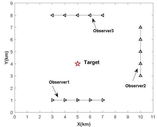
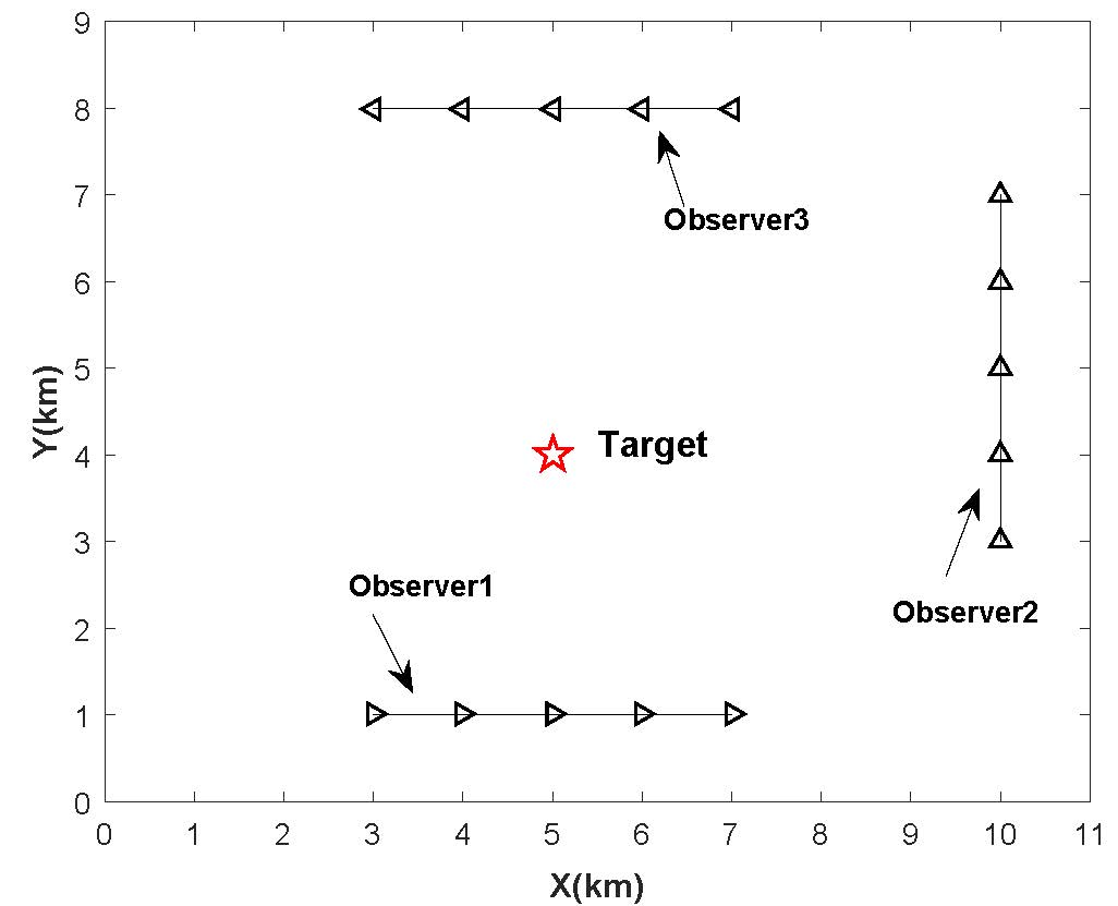
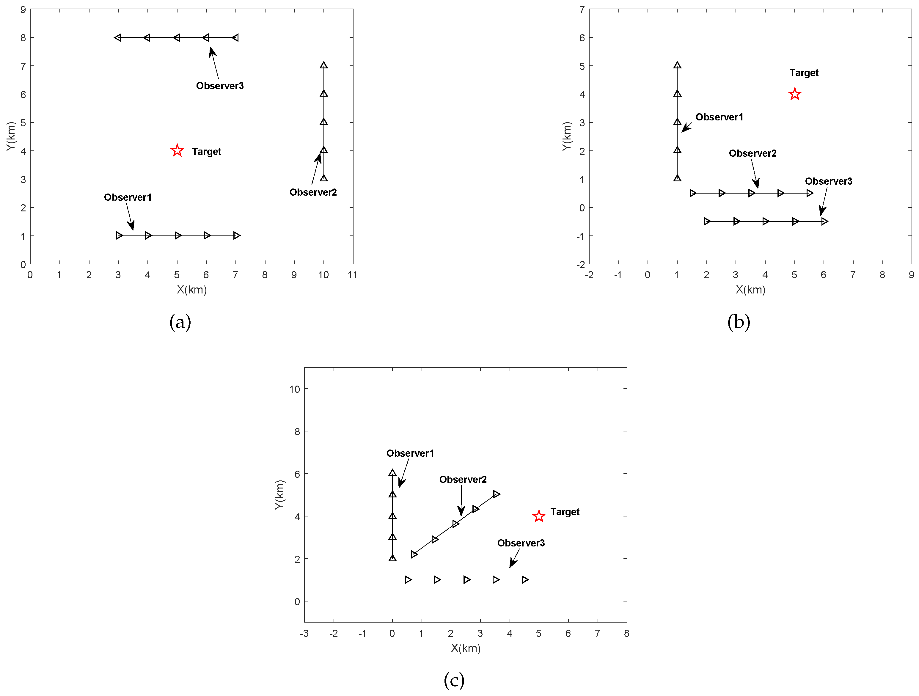
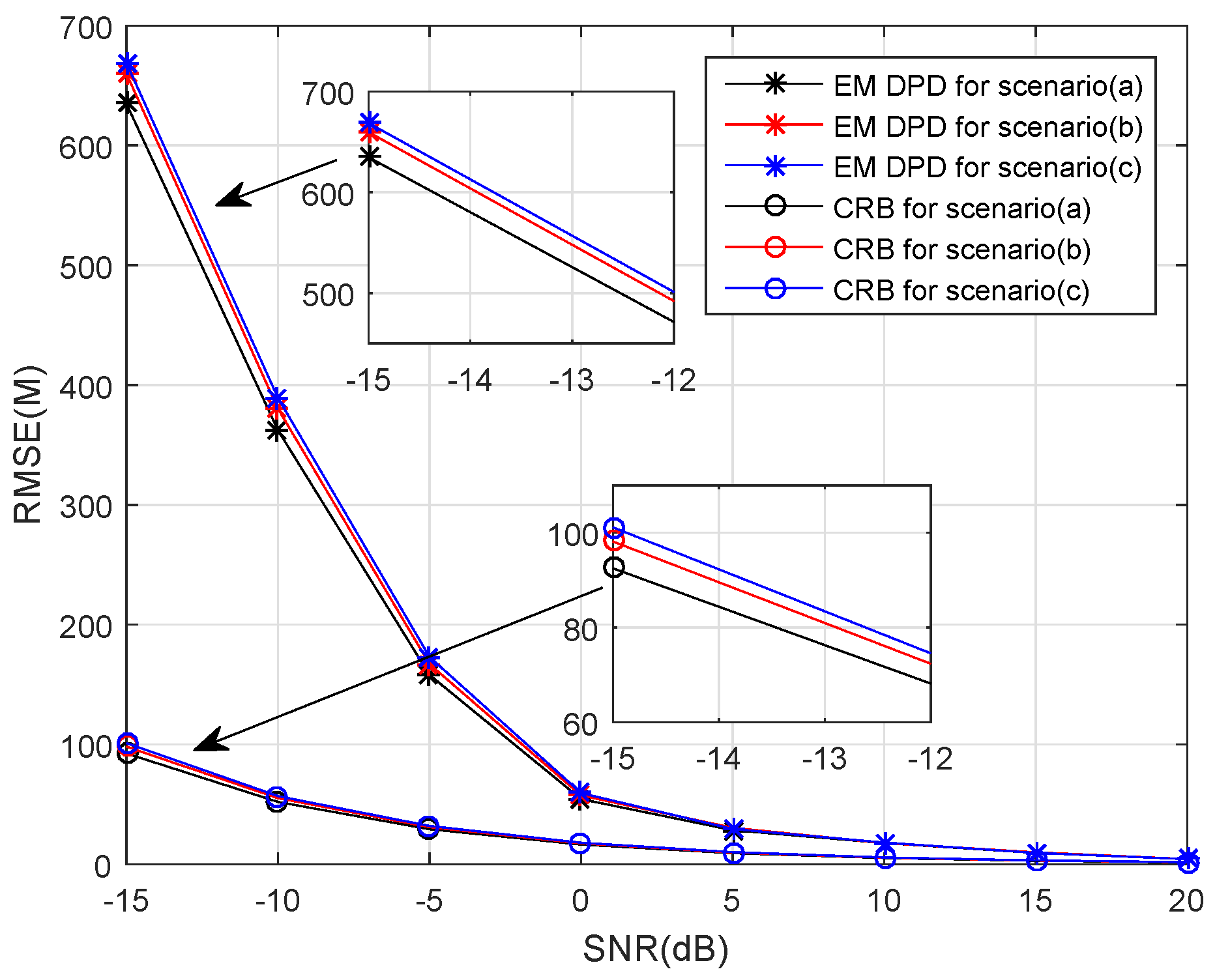
We now examine the localization performance of the proposed algorithm for three different scenarios. The target locates at [5, 4] km, and the receivers move along different trajectories, which can be found in Figure 1. As shown in Figure 2, the performance of our algorithm is not sensitive to the receiver trajectories because there is no significant difference between the RMSE curves of our algorithm for different scenarios. Additionally, as expected, the proposed method for Scenario (a) has better localization precision in low SNRs. On the other hand, although the RMSE of our algorithm is far from that of the corresponding CRB in low SNRs, it has a substantial advantage in computation time (see the descriptions for Table 4).
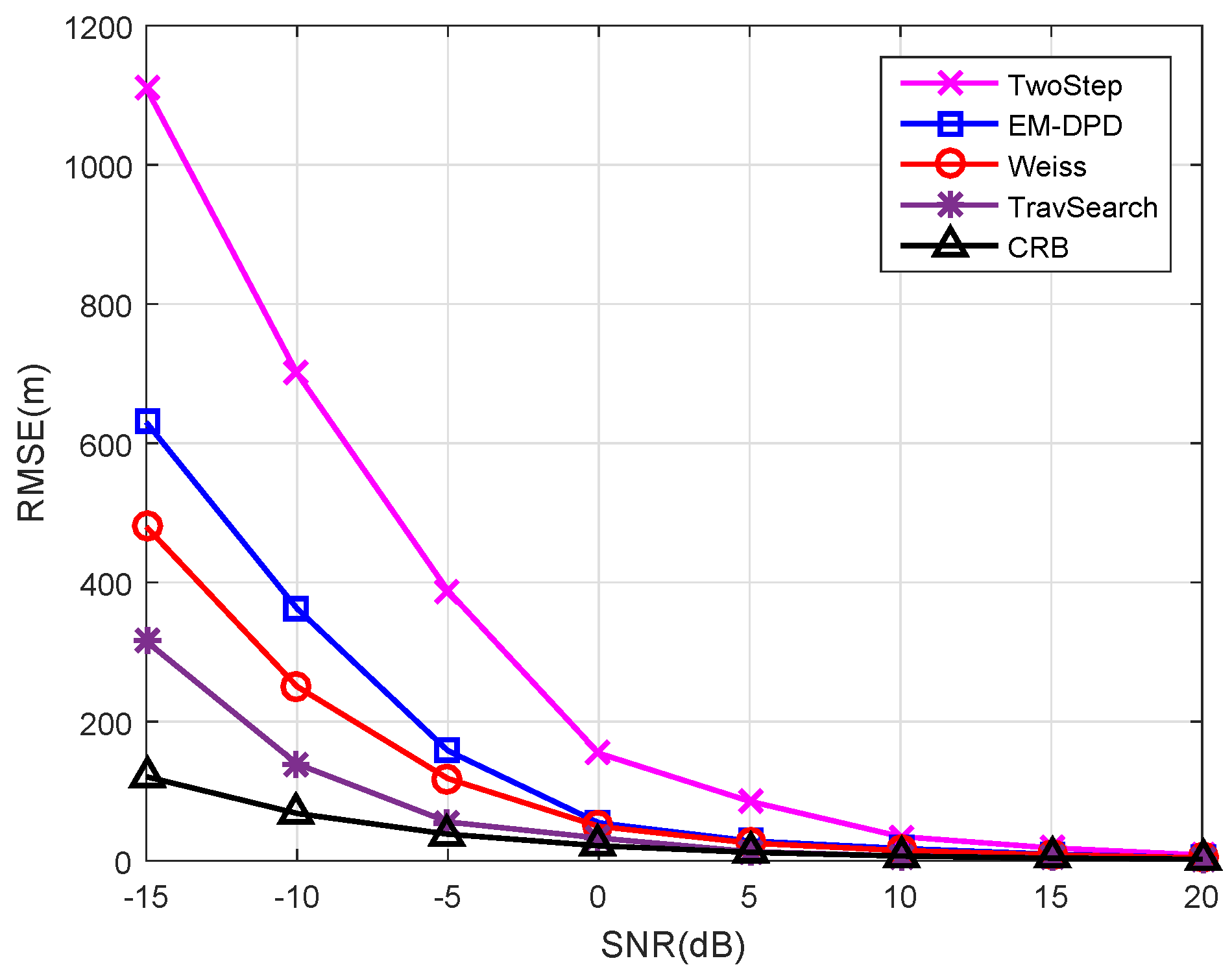
It must be emphasized that the next simulations are all based on Scenario (a) in Figure 1. Firstly, we continue to conduct the simulation for algorithm performance comparison versus SNRs. The RMSEs of all algorithms can be easily found in Figure 3. Unsurprisingly, all DPD methods outperform the two-step method, and the traversal search method shows the best localization performance especially in low SNRs. Although the performance of the proposed method is slightly inferior than that of Weiss’s method in low SNRs, it is more efficient. However, the other two DPD methods will cost a high amount of time in the presence of limited computing resources, losing its timeliness to moving target. The detailed runtime information can be seen in Table 4.
Secondly, to better exhibit the computational complexity of each algorithm, the runtime is investigated. From the results in Table 4, we observe that the two-step method requires the least runtime, but its localization performance is deteriorated in low SNRs (see Figure 3). Due to the high-dimensional search, the traversal search method is more computationally expensive than other DPD methods. Obviously, Weiss’s method has a great improvement in the running time. Compared with Weiss’s method, the run time of our method is further reduced (approximately 40%). However, the reduction of computational complexity of our method does not deteriorate localization performance significantly (also see Figure 3). As indicated by these finding, the proposed approach receives acceptable localization performance with a low computation resource cost.
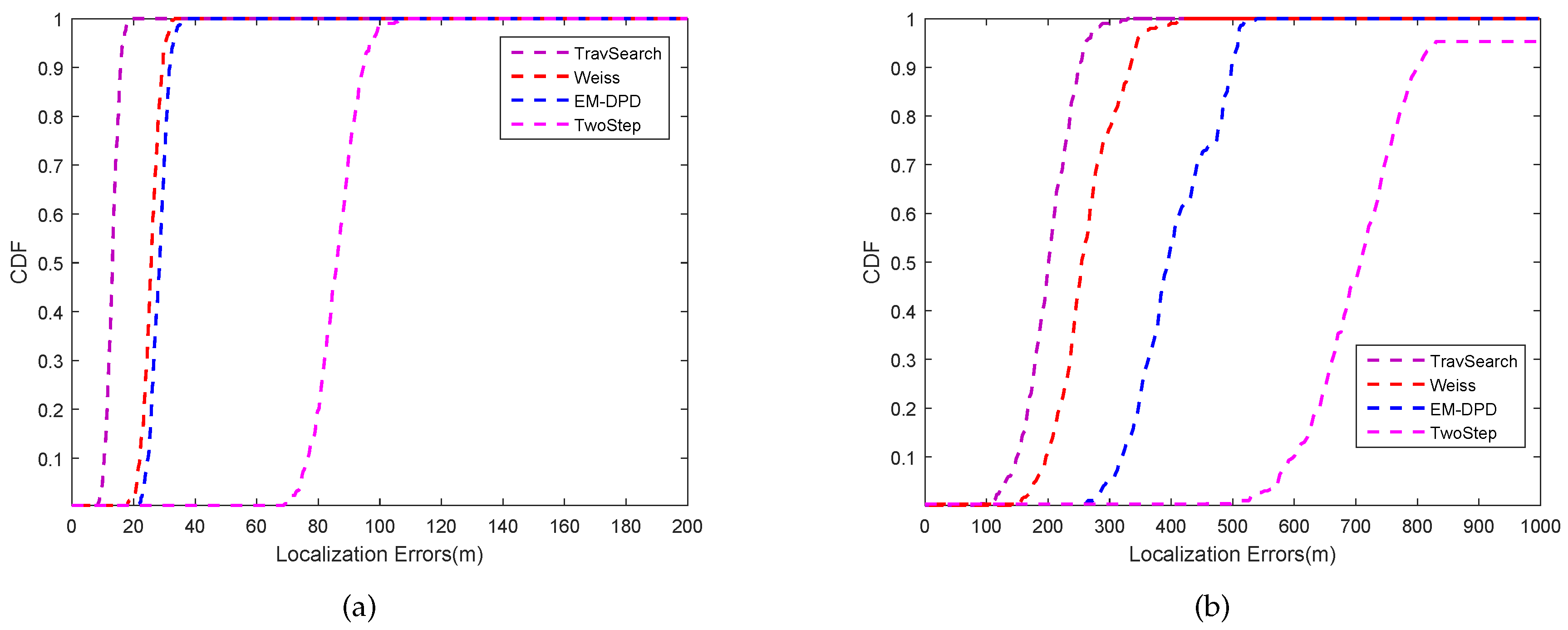
Thirdly, the CDF curves of all methods at the nominal constellation are depicted in Figure 4a,b at the SNR level of 5 dB and −10 dB, respectively. It can be readily observed that the traversal search curve is highest at a different localization error level. The proposed method curve is associated with Weiss’s DPD curve, which indicates it can receive high localization accuracy with high SNRs. From Figure 4, the two-step method curve deviates from the DPD methods. The proposed method curve is slightly apart from the curve of Weiss’s method, which is acceptable in terms of low complexity.
Finally, to further examine the influence of system parameter values on localization performance, we set SNR = −5 dB and exhibit the RMSE curves for K, N, L, and v in Figure 5, respectively. Additionally, the simulation conditions are K ranging from 2 to 10, N ranging from 50 to 200, L ranging from 1 to 6, and v ranging from 100 to 1000. It can be readily found in Figure 5a–c that all algorithms perform better in terms of localization accuracy, as more system parameter information exists. These results imply that the increase of these system parameters can enhance the localization performance. However, more parameter requirements mean greater system overhead and computational pressure. Consequently, our method can play an excellent role in the presence of limited computational resources. Furthermore, Figure 5d indicates that v does not have much impact on position accuracy.
6. Conclusions
The traditional two-step methods have high computational efficiency but low localization performance. To enhance positioning accuracy, DPD approaches have been developed. Since the DPD technology locates the target from the signal directly, computational complexity of this estimator is high. To solve this problem, this paper proposes a fast ML-based direct localization method using an EM algorithm based on time delay and Doppler shift. The EM scheme was developed to solve the ML problem in the DPD model. We simplify this ML problem via the theories of Gibbs inequality and Laplace approximation, transforming the high-dimensional nonlinear search into a few one-dimensional searches. Simulation results show that the proposed algorithm has operates faster than other DPD methods. Furthermore, when limited computing resources appear, our method leads a more efficient result on the basis of guaranteeing high localization accuracy. Therefore, compared with other localization approaches, the proposed method becomes a good way to balance localization accuracy and computational complexity.
Author Contributions
T.Q. derived the proposed method. T.Q. and L.L. conceived and designed the experiments. T.Q. and B.B. performed the simulations. D.W. analyzed the results. T.Q. wrote the paper. L.L. reviewed the paper.
Funding
The work was supported by the National Natural Science Foundation of China (grant no. 61401513).
Conflicts of Interest
The authors declare no conflict of interest.
Appendix A. Evaluation of xl,k and via Laplace Method
We consider the multivariate functions and . An integral is expressed by
Assume that has a global maximum within the interval. According to [27], the Laplace approximation is written as
where is the Hessian of at . Next we approximate the integral of and . For the sake of brevity, we omit in the subsequent derivation.
The expression of the conditional expectation is
The polar coordinates can be written as
Substituting (A4) into (A3) yields
where , and . We assume and have [28]
where , denote the first kind of modified Bessel function. We substitute Equation (A6) into Equation (A5), yielding
Recalling the expression in Equation (A2), we can search for the global extreme through
Therefore, we have
Similarly, we have .
Appendix B. Derivation of the Cramér–Rao Bound
It is well known that the CRB provides a benchmark for the best localization accuracy for any unbiased estimator. This section derives the compact CRB formula for source position with known signal waveforms and unknown transmitted time.
Let . According to [22], the th entry of the fisher information matrix of unknown parameter is shown as
For easy derivation, can be redefined by
where and . Thus, can be expressed by
Next we calculate the subblocks of Equation (A12).
Appendix B.1. The Partial of Dl,k (θ) with Respect to b
Note that is a complex variable, so we obtain
Appendix B.2. The Partial of Dl,k (θ) with Respect to t0
We obtain
where , with .
Appendix B.3. The Partial of Dl,k (θ) with Respect to p
We define with . The derivative with respect to can be expressed by
where
with
By substituting Equations (A13)–(A15) into Equation (A10), we can obtain the subblocks of
Since submatrices of Equation (A12) with respect to diagonal symmetry are transposed matrices of each other, we can easily obtain the remaining submatrices.
Thus, the inverse of the CRB of position can be obtained by
This concludes the derivation.
References
- Zhang, Y.; Xu, X.; Sheikh, Y.A.; Ye, Z. A rank-reduction based 2-D DOA estimation algorithm for three parallel uniform linear arrays. Signal Process. 2016, 120, 305–310. [Google Scholar] [CrossRef]
- Oh, D.; Kim, S.; Yoon, S.H.; Chong, J.W. Two-dimensional ESPRIT-like shift-invariant TOA estimation algorithm using multi-band chirp signals robust to carrier frequency Offset. IEEE Trans. Wirel. Commun. 2013, 12, 3130–3139. [Google Scholar] [CrossRef]
- Cao, H.; Chan, Y.T.; So, H.C. Maximum likelihood TDOA estimation from compressed sensing samples without reconstruction. IEEE Signal Process. Lett. 2017, 24, 564–568. [Google Scholar] [CrossRef]
- Tahat, A.; Kaddoum, G.; Yousefi, S.; Valaee, S.; Gagnon, F. A look at the recent wireless positioning techniques with a focus on algorithms for moving receivers. IEEE Access. 2016, 4, 6652–6680. [Google Scholar] [CrossRef]
- Gajewski, P.; Ziolkowski, C.; Kelner, J.M. Using SDF method for simultaneous location of multiple radio transmitters. In Proceedings of the 2012 19th International Conference on Microwave Radar and Wireless Communications (MIKON), Warsaw, Poland, 21–23 May 2012; IEEE: Warsaw, Poland, 2012; Volume 2, pp. 634–637. [Google Scholar]
- Kelner, J.M.; Ziolkowski, C.; Nowosielski, L.; Wnuk, M. Localization of emission source in urban environment based on the Doppler effect. In Proceedings of the 2016 IEEE 83rd Vehicular Technology Conference (VTC Spring), Nanjing, China, 15–18 May 2016; pp. 1–5. [Google Scholar]
- Yeredor, A.; Angel, E. Joint TDOA and FDOA Estimation: A Conditional Bound and Its Use for Optimally Weighted Localization. IEEE Trans. Signal Process. 2011, 59, 1612–1623. [Google Scholar] [CrossRef]
- Stein, A. Differential delay/Doppler ML estimation with unknown signals. IEEE Trans. Signal Process. 1993, 41, 2717–2719. [Google Scholar] [CrossRef]
- Viberg, M.; Ottersten, B. Sensor array processing based on subspace fitting. IEEE Trans. Signal Process. 1991, 39, 1110–1121. [Google Scholar] [CrossRef]
- Wang, Y.L.; Wu, Y. An efficient semidefinite relaxation algorithm for moving source localization using TDOA and FDOA measurements. IEEE Commun. Lett. 2017, 21, 80–83. [Google Scholar] [CrossRef]
- Park, C.H.; Chang, J.H. Closed-Form Localization for Distributed MIMO Radar Systems Using Time Delay Measurements. IEEE Trans. Wirel. Commun. 2016, 15, 1480–1490. [Google Scholar] [CrossRef]
- Xu, N.W.; Tang, C.N.; Wu, S.H.; Li, G.L.; Yang, J.Y. Optimal design of microseismic monitoring networking and rrror analysis of seismic source location for rock slope. Adv. Mater. Res. 2011, 163–167, 2991–2999. [Google Scholar]
- Papakonstantinou, K.; Slock, D. Direct location estimation using single-bounce NLOS time-varying channel models. In Proceedings of the 2008 IEEE 68th Vehicular Technology Conference, Calgary, BC, Canada, 21–24 September 2008; pp. 1–5. [Google Scholar]
- Demissie, B. Direct localization and detection of multiple sources in multi-path environment. In Proceedings of the 14th International Conference on Information Fusion, Chicago, IL, USA, 5–8 July 2011; pp. 1–8. [Google Scholar]
- Yin, J.X.; Wang, D.; Wu, Y.; Liu, R.R. A decoupled direct position determination algorithm for multiple targets in mixed LOS/NLOS environments. Acta Aeronaut. Astronaut. Sin. 2018, 39, 321338. [Google Scholar]
- Du, J.; Wang, D.; Yu, W.; Yu, H.; Du, J.; Wang, D.; Yu, W.; Yu, H. Direct position determination of unknown signals in the presence of multipath propagation. Sensors 2018, 18, 892. [Google Scholar]
- Weiss, A.J.; Amar, A. Direct position determination of multiple radio signals. EURASIP J. Appl. Signal Process. 2005, 1, 1–13. [Google Scholar] [CrossRef]
- Chen, L.; Zhang, H.; Sun, H. Multi-target direct position determination using subspace based compressive sensing. J. Signal Process. 2015, 31, 1272–1278. [Google Scholar]
- Weiss, A.J. Direct position determination of narrowband radio frequency transmitters. IEEE Signal Process. Lett. 2004, 11, 513–516. [Google Scholar] [CrossRef]
- Tzoreff, E.; Bobrovsky, B.Z.; Weiss, A.J. Single receiver emitter geolocation based on signal periodicity with oscillator instability. IEEE Trans. Signal Process. 2014, 62, 1377–1385. [Google Scholar] [CrossRef]
- Weiss, A.J. Direct geolocation of wideband emitters based on delay and Doppler. IEEE Trans. Signal Process. 2011, 59, 2513–2521. [Google Scholar] [CrossRef]
- Wang, D.; Zhang, G.; Shen, C.; Zhang, J. A direct position determination algorithm for constant modulus signals with single moving observer. Acta Aeronaut. Astronaut. Sin. 2016, 37, 1622–1633. [Google Scholar]
- Lu, Z.; Wang, J.; Ba, B.; Wang, D. A novel direct position determination algorithm for orthogonal frequency division multiplexing signals based on the time and angle of arrival. IEEE Access. 2017, 5, 25312–25321. [Google Scholar] [CrossRef]
- Reuven, A.M.; Weiss, A.J. Direct position determination of cyclostationary signals. Signal Process. 2009, 89, 2448–2464. [Google Scholar] [CrossRef]
- Huda, S.; Yearwood, J.; Togneri, R. A stochastic version of Expectation Maximization algorithm for better estimation of Hidden Markov Model. Pattern Recogn. Lett. 2009, 30, 1301–1309. [Google Scholar] [CrossRef]
- Katsaggelos, A.K. Image identification and restoration based on the expectation-maximization algorithm. Opt Eng. 1990, 29, 436. [Google Scholar] [CrossRef]
- Mada, K.K.; Wu, H.-C.; Iyengar, S.S. Efficient and robust EM algorithm for multiple wideband source localization. IEEE Trans. Veh. Technol. 2009, 58, 3071–3075. [Google Scholar] [CrossRef]
- Lu, L.; Wu, H.-C. Robust expectation-maximization direction-of-arrival estimation algorithm for wideband source signals. IEEE Trans. Veh. Technol. 2011, 60, 2395–2400. [Google Scholar] [CrossRef]
- Lu, L.; Wu, H.-C.; Yan, K.; Iyengar, S.S. Robust expectation-maximization algorithm for multiple wideband acoustic source localization in the presence of nonuniform noise variances. IEEE Sens. J. 2011, 11, 536–544. [Google Scholar] [CrossRef]
- Tzoreff, E.; Weiss, A.J. Expectation-maximization algorithm for direct position determination. Signal Process. 2017, 133, 32–39. [Google Scholar] [CrossRef]
- Yin, J.X.; Wang, D.; Wu, Y.; Tang, T. Single-step localization using multiple moving arrays in the presence of observer location errors. Signal Process. 2018, 152, 382–410. [Google Scholar] [CrossRef]
Figure 1.
The simulated localization scenarios: (a) scenario 1, (b) scenario 2, (c) scenario 3.

Figure 2.
The RMSE and Cramér–Rao bound (CRB) versus SNRs for different scenarios.

Figure 3.
The RMSEs of different algorithms versus SNRs.

Figure 4.
The CDF of different algorithms versus localization errors: (a) SNR = 5 dB; (b) SNR = −10 dB.
Figure 4.
The CDF of different algorithms versus localization errors: (a) SNR = 5 dB; (b) SNR = −10 dB.

Figure 5.
The RMSEs of different algorithms versus system parameters: (a) the value of K; (b) the value of N; (c) the value of L; (d) the value of v.
Figure 5.
The RMSEs of different algorithms versus system parameters: (a) the value of K; (b) the value of N; (c) the value of L; (d) the value of v.


Table 1.
Mathematical notation explanation.
| Notation | Explanation |
|---|---|
| transpose | |
| conjugate transpose | |
| the real part | |
| the imaginary part | |
| a diagonal matrix with diagonal entries | |
| ⊗ | Kronecker product |
| Euclidean norm of the matrix | |
| determinant of the matrix | |
| the joint distribution of and | |
| the conditional distribution of given | |
| identity matrix | |
| matrix with zero |
Table 2.
Computational complexity.
| Algorithm | Amount of Computation |
|---|---|
| Traversal search method | |
| Weiss’s method | |
| Proposed method |
Table 3.
Algorithms.
| Algorithm | Method |
|---|---|
| TOA/Doppler two-step method | Method in [2] to estimate TOA; Method in [8] to estimate Doppler; Least square (LS) location using the TOA and Doppler estimations. |
| Traversal search method | Method in [17] using a three-dimensional search |
| Weiss’s method | Method in [21] using eigenvalue decomposition |
Table 4.
Mean runtime of different methods.
| Algorithm | Runtime (s) |
|---|---|
| Two-step method | 0.8 |
| Traversal search method | 67 |
| Weiss’s method | 7.9 |
| Proposed method | 4.7 |
© 2018 by the authors. Licensee MDPI, Basel, Switzerland. This article is an open access article distributed under the terms and conditions of the Creative Commons Attribution (CC BY) license (http://creativecommons.org/licenses/by/4.0/).
Share and Cite
MDPI and ACS Style
Qin, T.; Li, L.; Ba, B.; Wang, D. A Fast ML-Based Single-Step Localization Method Using EM Algorithm Based on Time Delay and Doppler Shift for a Far-Field Scenario. Sensors 2018, 18, 4139. https://doi.org/10.3390/s18124139
AMA Style
Qin T, Li L, Ba B, Wang D. A Fast ML-Based Single-Step Localization Method Using EM Algorithm Based on Time Delay and Doppler Shift for a Far-Field Scenario. Sensors. 2018; 18(12):4139. https://doi.org/10.3390/s18124139
Chicago/Turabian StyleQin, Tianzhu, Lin Li, Bin Ba, and Daming Wang. 2018. "A Fast ML-Based Single-Step Localization Method Using EM Algorithm Based on Time Delay and Doppler Shift for a Far-Field Scenario" Sensors 18, no. 12: 4139. https://doi.org/10.3390/s18124139
Note that from the first issue of 2016, this journal uses article numbers instead of page numbers. See further details here.