Reliability and Maintenance Analysis of Unmanned Aerial Vehicles ^†

Abstract

This paper focuses on the development of a new logistic approach based on reliability and maintenance assessment, with the final aim of establishing a more efficient interval for the maintenance activities for Unmanned Aerial Vehicles (UAV). In the first part, we develop an architectural philosophy to obtain a more detailed reliability evaluation; then, we study the intrinsic reliability at the design stage in order to avoid severe critical issues in the UAV. In the second part, we compare different maintenance philosophies for UAVs and develop the concepts of preventive and corrective maintenance that consider the system subjected (until real “hard failure”) to partial performance degradation (“soft failure”). Finally, by evaluation of the uncertainty through the confidence interval, we determine the new soft failure limits, taking into account the general knowledge of the systems and subsystems in order to guarantee the proper preventive maintenance interval.

1. Introduction

The problem of reliability of UAVs, like problems of maintenance and safety, have become extremely important in recent years: engines became more robust, avionics was improved, etc. Despite this, the approach regarding the reliability of drones is still too fatalistic.

Obviously, by means of reliability analyses which are available nowadays, we consider that the absence of a driver or person on board does not allow us to design and realize the UAV with less stringent standards with respect to those used for airplanes. The commercial aviation failure rate is about 1/10⁵ flight hours, while for drones, it has been verified at about 1/10³ flight hours, so a higher magnitude of two orders. From a different point of view, sophisticated UAV systems have an overall failure rate of 25%. The aim of the paper, which is an extended version of [1], is to provide new ideas to increase the reliability of a drone optimizing maintenance activities. For this, we start from the philosophy of apportioning the percentages of reliability assigned (on average) to each system (and subsystem), trying to optimize them according to safety requirements. On the other hand, it is necessary to optimize the time intervals (and consequently the costs) of maintenance, taking into account that all critical systems must absolutely support preventive maintenance criteria: in these cases, we are helped by the concepts of soft and hard failure [2,3].

1.1. Definitions

Here, we will introduce a series of definitions which will be used throughout the paper.

1.1.1. Reliability

Reliability is a dynamic concept which is applicable to many fields, i.e., is not only strictly technical. For it, a possible definition could be expressed in terms of probability, and in particular, as “the probability that a system, subsystem or part is able to perform its specific function in a pre-established time and under pre-established conditions”. One of the most important reliability metrics is represented by the Mean Time Between Failures (MTBF), expressed in hours of activity; the higher the value, the more reliable the equipment. For a part or a single subsystem, the MTBF is often expressed as the reciprocal of reliability. For instance, the MTBF gives information about the level of unreliability, and it typically shows the number of failures of a piece of equipment over an established time, i.e., 10,000 h [4].

The Failure In Time (FIT) rate of a device represents the number of expected failures in one billion (10⁹) device-hours of operation. This parameter is widely diffused in the semiconductor industry [5,6,7] and international standards.

1.1.2. Availability

This parameter is extremely important for ‘ready to operate’ system. It measures the number of times for which the system under study is available or ready with respect to the number of times in which the system is required. Typically, this parameter is presented in form of a percentage, where 100% is the theoretical goal [8,9,10,11].

1.1.3. The Environment

According to “MIL-HDBK-217F2”, [12] (see

Table 1. Environment definition.

Class 1	Definition 1
AUF Airborne, Uninhabited, Fighter	Environmentally uncontrolled areas, which cannot be inhabited by an aircrew during flight. Environmental extremes of pressure, temperature and shock may be severe.

¹ Source: MIL-HDBK-217F2.

), the following operative environment is considered for the reliability prediction:

2. RAMS Assessment

The Reliability, Availability, Maintainability, and Safety (RAMS) assessment is an important study in the development of UAVs. This kind of analysis is mandatory if you want to increase the reliability of a drone, its availability, and to reduce repair and maintenance costs [13]. Once an architecture has been chosen, the RAMS assessment is very useful to identify all the critical elements that could increase the failure rate [14]. It also allows us to characterize all the most stressed (or undersized) areas of the project. Furthermore, the reliability prediction, for example, makes it possible to decide whether to duplicate a safety critical system or to put it in derated conditions, with great savings in terms of weight and power consumption [15,16,17,18,19]. A comparison between the well-known but always efficient technique of redundancy and the improvement of reliability must consider important remarks such as norms, costs, limitations of spaces, and so on. The reliability analysis helps us to assess the value of failures [20]. For instance, if some failures of a specific component happen in a wider system, the failure rate, preventively predicted, is useful to establish if the number of failures which is adequate to the overall number of components present in the system. Alternatively, it can individuate a particularly problematic section [21,22,23,24]. Finally, this kind of evaluation can be used to assess the probabilities of findable damage events in a FMECA (Failure Modes, Effects and Criticality Analysis).

3. How Reliable Does a Drone Have to Be?

During a typical mission, some failures are more critical than others: the loss of longitudinal stability, the loss of payload data, or the turning off of the position lights are not of the same criticality level. Therefore, it is necessary first to establish various levels of increasing gravity associated with the fault [25]. Moreover, according to the specific kind of mission and the specific kind of UAV, it is necessary to subdivide failures into subcategories [26]. Then, for each scenario, suitability and preventively forecasted, it is necessary to define a minimum acceptable level of reliability. Finally, even for the aircraft, it is necessary to define the criteria for the level of reliability, in terms of a level which is strictly linked to the type of failure [27,28,29,30,31].

• Catastrophic failures: for these kind of failures, a crash of the drone is certain while injuries or even the death of persons on the ground is possible.
• Severe failures: heavy damages are expected and the probability of repairing the drone is low.
• Moderate failures: cause a moderate degradation of the drone’s functions, which could lead to aborting the mission; however, they are not cause of severe damage.
• Soft failures: cause light degradation of the drone’s functions, but do not lead to the cancellation of the mission.

The intrinsic reliability of an apparatus (in our case, a drone) is the reliability studied a priori [32]; however, unfortunately, a reliability study is often realized after the design phase. This approach can lead to many problems during the management of the project, because a reliability study highlights a series of sensible points, and produces a series of recommendations that are usually forwarded to the designers. These should allow them to carry all the necessary modifications to the project in order to improve it [33,34,35,36,37,38]. The perspective is completely different in the case of intrinsic reliability: in fact, the knowledge of the failure distribution of a system gives rise to the possibility, directly during the design stage, of taking specific action to reduce criticality and upgrade the critical parts or subsystems in advance, thereby increasing the overall level of reliability [39]. This, surely, increases the level of responsibility of the designers, but at the same time, decreases the risk of criticalities (also called Single Point Failures or briefly SPF) that might happen in future studies [40,41,42,43].

This way of seeing the design phase, i.e., in which a reliability study is effectively used to help the project, means that the figure of the Quality Assurance Responsible is frequently present from the beginning. Reliability analyses primarily aim to find the minimum limits for the requirements that allow UAVs to have at least a magnitude of better reliable [44].

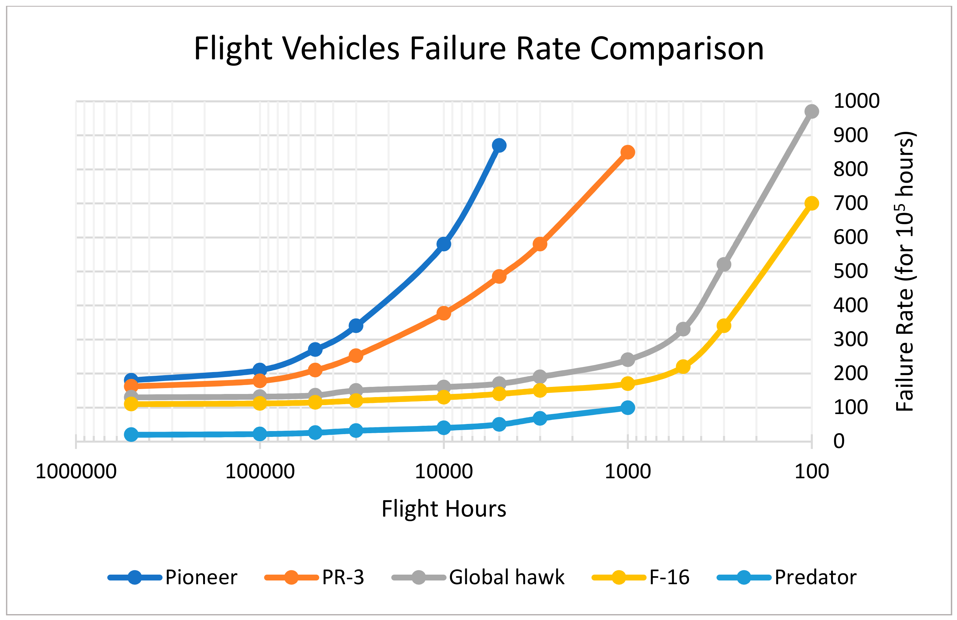
Another benefit of these analyses is that they help us to understand which components or parts of a specific subsystem are the most unreliable, and which are the most critical to the system [45,46,47,48,49,50]. In Figure 1 a failure rate comparison between five different aircrafts is shown: Northrop Grumman RQ-4 Global Hawk in gray, PR-3 in orange, General Atomics RQ-1 Predator in blue, AAI RQ-2 Pioneer (for the drone category) in light blue and General Dynamics F-16 jet fighter in yellow.

4. Reliability Assessment Hierarchy

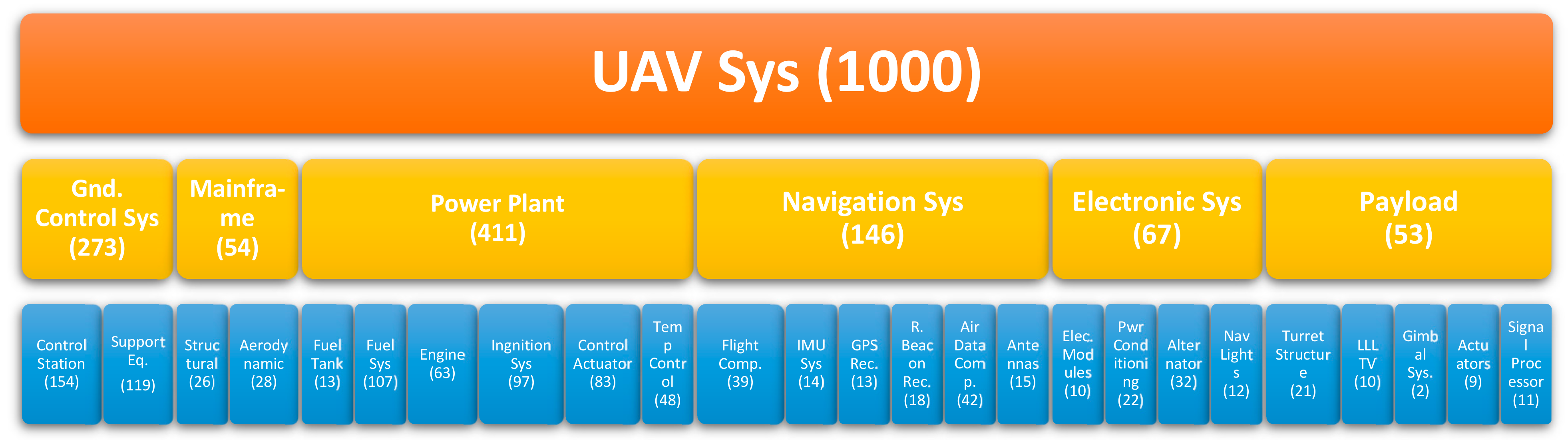
Considering all the possible main systems and subsystems that form an UAV, Figure 2 depicts the UAV hierarchy of the reliability assessment, showing their failure distribution every 10³ faults [51,52].

The following subparagraphs show how the failures are categorized, taking into account the function of each subsystem.

4.1. Ground Control System (GCS)

The Ground Control System, also called GCS, is the part with the highest maintainability of the whole UAV system; this is because it is easily accessible at any time during the mission. It is mainly composed of COTS (Commercial Off-The-Shelf) components with large inventories. This does not mean that it is less safe; the fact that it is ground-based allows the introduction of a good percentage of redundant systems with hot and cold stand-by configurations, reducing the off-line time nearly to zero [53].

4.2. Mainframe

The UAV mainframe is by far the strongest part of the whole system; this is designed with great attention by means of CAD systems, which allow the developers to study and evaluate the loads of the structure a priori. In general, the mainframe is appropriately oversized; in fact, even if this leads to extra weight, it is undoubtedly a small price to pay for a safer structural system. Generally, the most common failures occur due to fatigue cycles, soldering brazing, or untreated rivets [54].

4.3. Power Plant

The power plant itself is a rather reliable mechanical system, even if the subsystems could show some breakdowns. Especially in long-term missions, insufficient fuel vaporization or poor cooling can lead to overheating of the engine, or fatigue that could eventually lead to failure [55,56].

4.4. Navigation System

This system is the most important part of the vehicle; it is characterized by a high failure rate compared to other systems. Nevertheless, it has the highest number of hot redundant subparts/subsystems. Therefore, due to the high level of electronic miniaturization, it is possible to replicate a large number of its subsystems [57] making it intrinsically reliable. The Hot (standby) redundancy is a method in which one system runs simultaneously with an identical primary system. Upon failure of the primary system, the hot standby system immediately takes over, replacing the primary system.

Moreover, due to the strong integration derived from the experience of the development of automotive applications, the aerospace world enjoys highly-reliable electronic components for navigation (as Inertial Navigation System—INS and Global Positioning System—GPS receivers). A second benefit comes from their high computing capacity that allows a parallel computing architecture, greatly increasing the overall reliability [58].

4.5. Electronic System

In the previous discussion, we have deliberately separated the electronic system from the navigation system. Even from a purely mechanical point of view, it may not be so evident how they are separated from a functional and philosophical point of view. In fact, in order to prevent possible interference, the electronic system separates all the electronic circuits which are not closely related to navigation, such as the power supply and conditioning, to manage the telecommunication system to the outside (satellite communications, ground-vehicle data links, etc.). Even in this case, the hypothesis of redundancy has to be avoided because, for example, the weight of the harness would be excessively high for such a small vehicle [59].

4.6. Payload

The payload is not contained in its own conditioned bay inside the fuselage, but is placed outside in a mobile turret inserted directly in the aerodynamic flow. The turret itself contains several electro-optical sensors like a thermal imaging camera, a Low Light Level Television, a laser tracer etc. From a mechanical point of view, the turret is gimballed, allows ± 90° elevation, and 360° of continuous azimuth rotation; the system also contains the ancillary electronics of the sensors and the movement actuators.

The turret is thermostatically controlled to ensure optimal operation of the electronics and to prevent freezing of the kinematic devices in high-altitude flight conditions. For these applications, the electronics will be chosen with consideration of their intrinsic reliability and highest temperature operative range. The geometry of the cases of the components must be chosen carefully, as the aircraft is subjected to frequent and abrupt changes in altitude, and therefore, pressure, that could stress some components. It’s important to note that to put all the equipment into a sealed and pressurized container would be too burdensome from the point of view of weight.

5. Multiplexed Systems

Redundancy of the most critical systems does not always lead to an increase in the reliability of the whole system. In fact, the redundancy of a quite unreliable system means increases in the total failure rate. In other words, the overall safety of the system will be increased, but certainly not the reliability. A higher failure rate brings an increase in expenses for spare parts and in person-hours, increasing operating costs [11].

On the other hand, the duplication of the most critical or vital systems is not the ideal solution, as it increases the cost and the complications of the system, so it is necessary to find another way to improve reliability [60].

A classic case is that related to propulsion systems: many UAVs have only one engine, but this is a highly reliable system, even if its loss compromises the entire mission. The installation of two engines would seem to be an ideal solution because the loss of one of these would not compromise the final mission. However, the duplication of a motor means the duplication of all ancillary systems. This in turn leads to a decline in the system’s overall reliability [61].

The ideal solution is based on two keywords: oversize and derating. We will therefore choose an engine with characteristics that exceed the UAV requirements, and will work under ordinary operating conditions, i.e., derated, or in a very “relaxed” way. In this case, we will see that, while remaining a single point failure according to FMECA analysis, the engine has a considerably higher reliability, as it will work at less than 50% of its capability; this condition reduces the rate of failure occurrence.

6. The UAV as a Complex Maintenance System

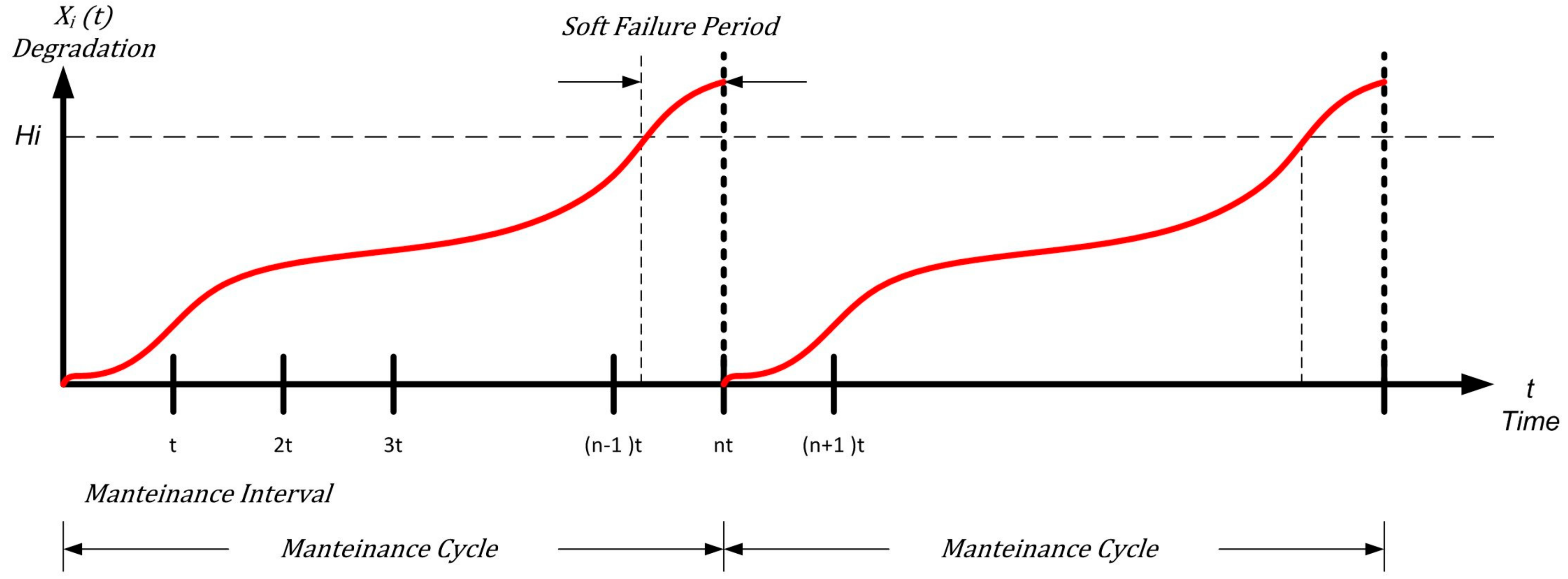
Now we consider an UAV as a complex aerial system composed by m subsystems (or subparts) defined as J = {1, 2, …, m}, and consisting of l_j components. At the component level, we can continuously control and check the degradation of a defined collection of physical parameters. The physical conditions degrade monotonically during use, and are restored by maintenance actions. For each component or subpart i ∈ I, X_i(t) indicates the degradation trajectory in a fixed time interval t ∈ [0, ∞). Soft failure can be defined as the ability of a component, part, subsystem or system to continue its work even if with degraded performance, i.e., up to the point when its reduced performance exceeds a specific fixed threshold H_i (with X_i(t) > H_i), called soft failure one. Typically, components subjected to thermal stress or mechanical degradation are hit by soft failures.

When X_i(t) exceeds H_i, a soft failure happens between two maintenance points (n − 1)τ and nτ. This implies an action of corrective maintenance (CM), which has a specific cost (c_i^CM) on the critical component. This action is executed in a fixed time called maintenance point nτ, as shown in Figure 3.

The period between the occurrence of the soft failure point and the maintenance point nτ is defined as “soft failure period”. This period defines loss of quality in production or poorer performance with a cost rate indicated with c_i^P [61].

6.1. Degradation Model for an UAV

In this section, starting from the UAV degradation model, we will arrive at defining limits and probabilistic criteria to determine the optimal maintenance interval that does not exceed the corrective maintenance threshold: maintenance that yields effect when the gradual damage is intolerable by the agreed-upon operational standards.

The random coefficient model is used to evaluate the level of degradation for the ith component for a time $\widehat{t}$∈[0, ∞) in a cycle of single maintenance Φ_i = {ϕ_i,1, …, ϕ_i,Q}, Q ∈ $\mathbb{N}$, then a set of random parameters Θ_i = {θ_i,1, …, θi_,V }, V ∈ $\mathbb{N}$ following a normal (Laplace–Gauss) distribution [62].

The probability that the degradation at time $T_{\chi }$ reaches the threshold $\chi$ before time $\widehat{t}$ is:

$$P_r\left\{T_{\chi }< \widehat{t}\right\}= P_r\left\{X\left(\widehat{t} ;{\Phi }_i,{\Theta }_i \right)>\chi \right\}, \forall i\in I$$

(1)

The calculation of this probability is necessary because, in the next discussion, we will introduce a certain degradation profile and calculate the probability that this has to overcome the various critical failure thresholds.

We consider a complex system with the following degradation path (this type of degradation has been chosen because it is typical of this kind of complex systems):

$$X_i \left(t, {\Phi }_i,{\Theta }_i\right)={\varphi }_{i,1}+{\theta }_{i,1}·{\widehat{t}}^{{\varphi }_{i,2}}$$

(2)

where ${\Phi }_i=\left\{{\varphi }_{i,1}, {\varphi }_{i,2}\right\}$ and ${\Theta }_i=\left\{{\theta }_{i,1}\right\}$ then:

$$P_r\left\{T_{\chi }<\widehat{t}\right\}= P_r\left\{{\varphi }_{i,1}+{\theta }_{i,1}·{\widehat{t}}^{{\varphi }_{i,2}}>\chi \right\}$$

(3)

$$P_r\left\{T_{\chi }<\widehat{t}\right\}= P_r\left\{{\theta }_{i,1}>\frac{\chi - {\varphi }_{i,1} }{{\widehat{t}}^{{\varphi }_{i,2}}}\right\}$$

(4)

For a random variable, ${\theta }_{i,1}\ge 0$, we evaluate the cumulative density function $F_{{\theta }_{i,1}}$:

$$P_r\left\{T_{\chi }<\widehat{t}\right\}= 1- F_{{\theta }_{i,1}}\left(\frac{\chi - {\varphi }_{i,1} }{{\widehat{t}}^{{\varphi }_{i,2}}}\right)$$

(5)

Now we evaluate the probability in which, between the two time points (n − 1)τ and nτ, the control limit C_i is reached:

$$P_r\left\{X_i\left(\left(n-1\right)\tau ; {\Phi }_i,{\Theta }_i\right)\right\}\le C_i<X_i\left(n\tau ;{\Phi }_i,{\Theta }_i \right), \forall n\in \mathbb{N}$$

(6)

that is equal to:

$$P_r\left\{\left(n-1\right)\tau \right\}\le T_{C_i}<n\tau , \forall n\in \mathbb{N}$$

(7)

The soft failure threshold H_i is reached before time point nτ only if it has satisfied the following condition:

$$P_r\left\{X_i\left(n\tau ;{\Phi }_i,{\Theta }_i \right)>H_i\right\}=P_r\left\{T_{H_i}<n\tau \right\}, i\in I$$

(8)

Moreover, assuming the degradation path as monotonic (typical of this kind complex systems), we have: C_i < H_i with and $T_{C_i}\le T_H$.

6.2. Uncertainty of Degradation in Corrective Maintenance

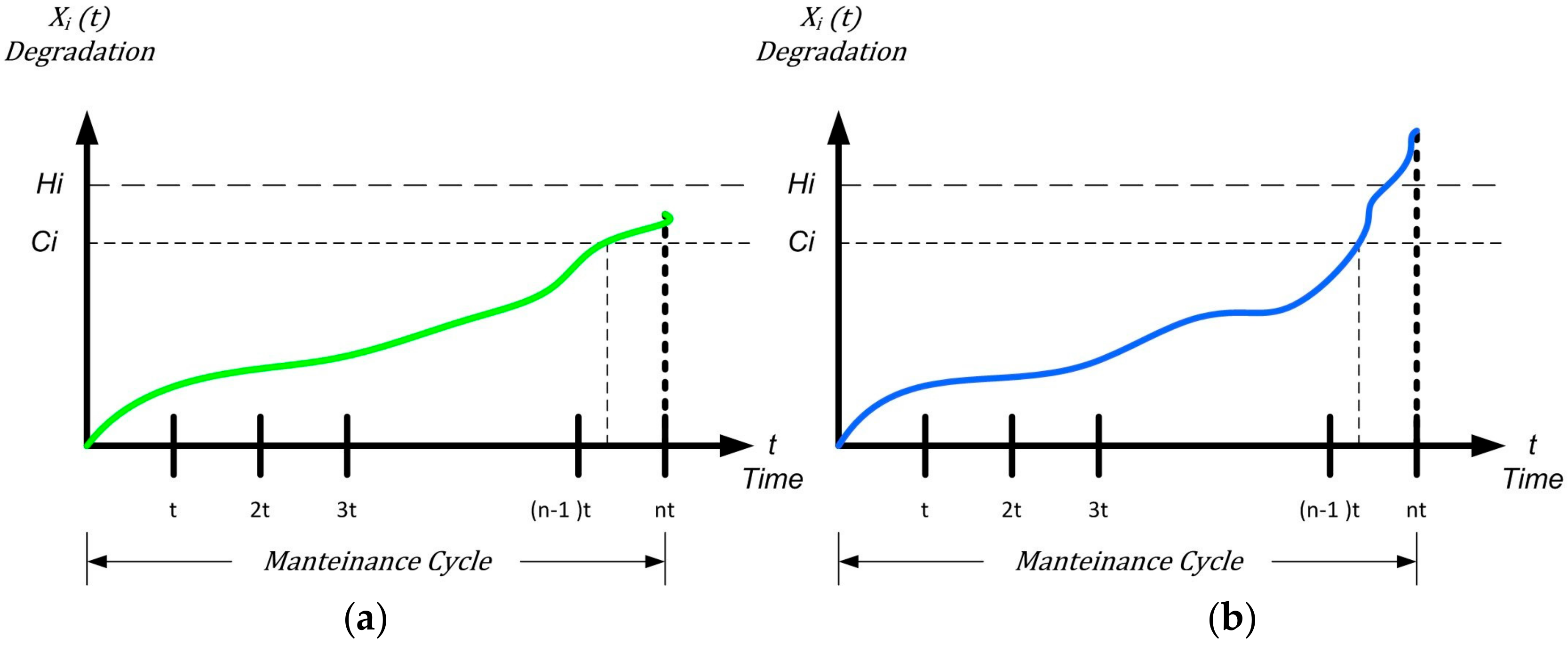
If $\left(n-1\right)·\tau \le C_i<n\tau$ we have two occurrences for the maintenance decision at time nτ: preventive maintenance (PM) (see Figure 4a) and corrective maintenance (CM) (see Figure 4b) according to:

$$\{\begin{array}{l}Preventive if: C_i \le X_i\left(n\tau \right)<H_i\\ Corrective if: X_i\left(n\tau \right)\ge H_i\end{array}$$

(9)

The probability that a preventive maintenance happens at the specific time nτ after the degradation level of the ith component has reached the control limit $\left(n-1\right)·\tau \le C_i<n\tau$ is [63]:

$$P_r\left\{PM at n\tau \right\}= P_r\left\{T_{H_i}>n\tau , \left(n-1\right)\tau \le T_{C_i}<n\tau \right\}$$

(10)

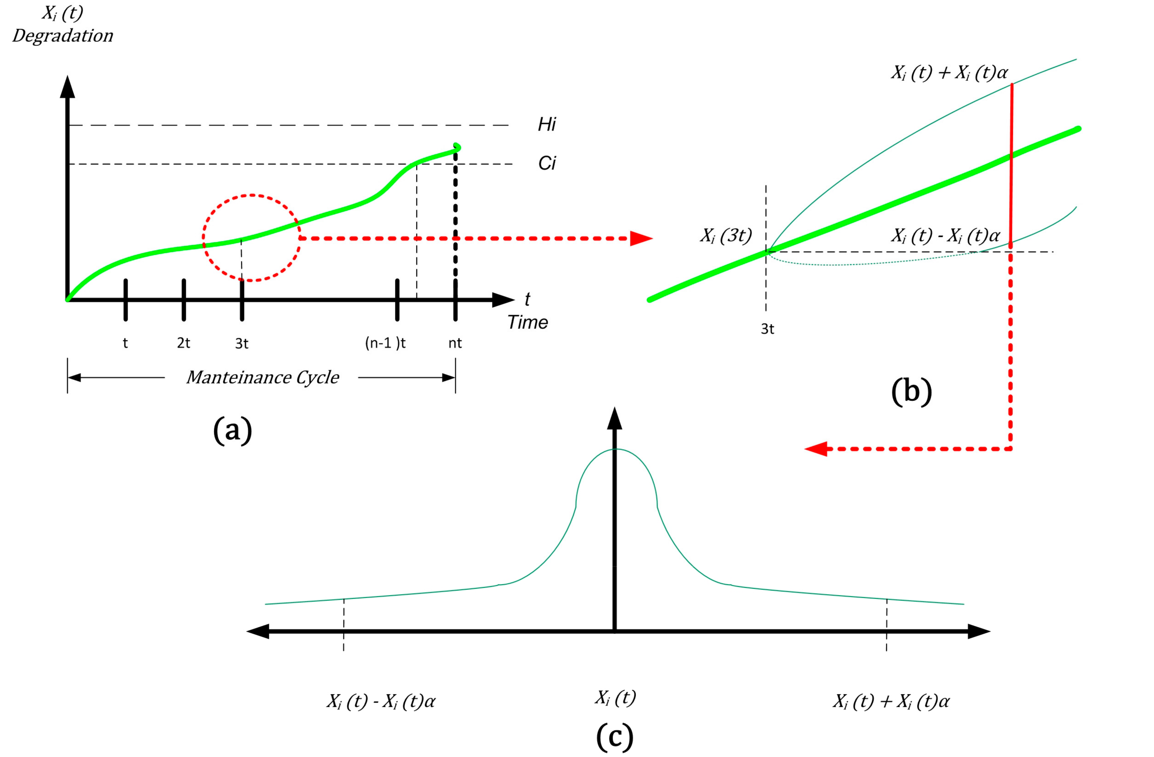
Now we consider the monotonic expression in the preventive maintenance: consider, for example, what is happening around the monotone function immediately after the 3t maintenance interval (see Figure 5a).

After the maintenance interval, since one of the returns from the field of intervention is the degradation state of the systems and subsystems, we know exactly what the degradation status of the systems and subsystems is. In other words, we can quantify as X_i(3t) as the status of the probability at the moment we are studying.

Immediately after the “3t moment”, we have a view of the drift in time of the value: a band of uncertainty affects the probabilistic function (supposedly monotonous). The uncertainty is due to the capability of controlling the state of degradation of systems (and subsystems) limited by our confidence interval (see Figure 5a–c) in terms of knowledge of the complete system.

Now we consider X₁, …, X_n as samples of the subsystems degradation status of normal density after the revision X_i(3t) with unknown mean m and variance σ² (known) and sample average $\overline{X}$. We have:

$$\underset{Xi\left(t\right)-Xi\left(t\right) \alpha }{\overset{Xi\left(t\right)+Xi\left(t\right) \alpha }{{\displaystyle \int }}}\frac{1}{\sqrt{2\pi }}{e}^{\frac{Xi\left(t\right){ }^2}{2}} dX =Xi\left(t\right) \left(1-\alpha \right)$$

(11)

Therefore, we have:

$$Xi\left(t\right)\left(1-\alpha \right)= P_r\left\{\left|\frac{\sqrt{n}}{\sigma }·\left(\overline{X}-m\right)\right|\le Xi\left(t\right) \alpha \right\}$$

(12)

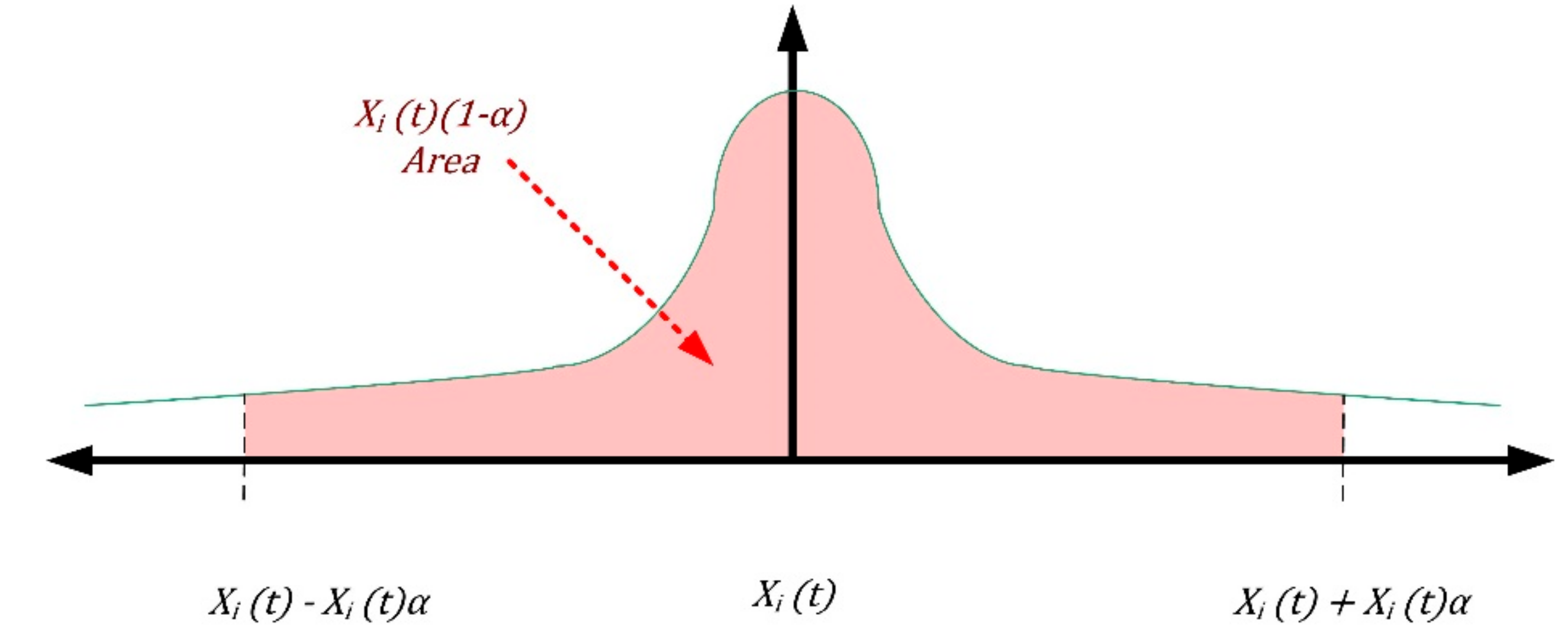
Explaining the second member (see Figure 6):

$$Xi\left(t\right)\left(1-\alpha \right)= P_r\left\{\overline{X}- \frac{\sigma }{\sqrt{n}}·Xi\left(t\right)\alpha \le m \le \overline{X}+ \frac{\sigma }{\sqrt{n}}·Xi\left(t\right) \alpha \right\}$$

(13)

We have for the confidence interval of level $Xi\left(t\right)\left(1-\alpha \right)=$ for m:

$$\left[\overline{X}- \frac{\sigma }{\sqrt{n}}·Xi\left(t\right)\alpha ,\overline{X}+ \frac{\sigma }{\sqrt{n}}·Xi\left(t\right) \alpha \right]$$

(14)

It is necessary to treat the limitation of this method: the term $Xi\left(t\right)-Xi\left(t\right) \alpha$ can never be lower than X_i(3t). This is because the system, despite monotonic evolution in a more optimistic than linearized way (Figure 5b—green line), cannot, for logical reasons of entropy, improve over time, or have a negative degradation. This condition is only theoretically possible, and is due to the uncertainty of the state of knowledge of the system. Therefore, to restore the physical consistency of the uncertainty evaluation, it is necessary to add the condition:

$$\{\begin{array}{c}\left[\overline{X}- \frac{\sigma }{\sqrt{n}}·Xi\left(t\right)\alpha ,\overline{X}+ \frac{\sigma }{\sqrt{n}}·Xi\left(t\right) \alpha \right]\\ Xi\left(3t\right)\le Xi\left(t\right)-Xi\left(t\right) \alpha \end{array}$$

(15)

Our prediction of the state of health of our system cannot disregard the knowledge of the state of the subsystems: their number and state influence the possible uncertainty of the value X_i(t).

6.3. The Thresholds of Preventive Maintenance

Considering the above calculations, when we want to evaluate the occurrence of the preventive maintenance intervals, we need to consider the confidence interval in terms of knowledge of the subsystems.

Reconsidering the confidence interval and the n cycle, the second part of the expression (9) becomes:

$$Xi\left(nt\right)+Xi\left(nt\right) \alpha <H_i$$

(16)

Obviously, the real problem happens when the threshold $H_i$ is exceeded:

$$Xi\left(nt\right)+Xi\left(nt\right) \alpha <H_i$$

(17)

so:

$$Xi\left(nt\right) \left(1+\alpha \right)<H_i$$

(18)

And the new sof failure limit is:

$$Xi\left(nt\right) <\frac{H_i}{1+\alpha }$$

(19)

Therefore, it is necessary to keep the confidence interval as narrow as possible.

Knowledge of the subsystems is therefore essential for evaluation: we risk calculating the total reliability of the system without evaluating the total accuracy that, in the worst case, would lead to a wrong assessment of preventive maintenance or an incorrect evaluation of preventive maintenance. Obviously, this is an undesirable situation.

The condition for the threshold $C_i$ is:

$$C_i \le Xi\left(nt\right)-Xi\left(nt\right) \alpha$$

(20a)

so:

$$C_i \le Xi\left(nt\right) \left(1-\alpha \right)$$

(20b)

and:

$$\frac{ C_i }{1-\alpha } \le Xi\left(nt\right)$$

(21)

Now, the first member of the (9) becomes:

$$\frac{ C_i }{1-\alpha } \le Xi\left(nt\right) <\frac{H_i}{1+\alpha }$$

(22)

Now we can objectively quantify the level of accuracy needed to define the preventive maintenance intervals.

It is still useful to specify the function from a graphical point of view. Now consider the upper zone of Figure 4a in detail (see Figure 7):

From Figure 7a, the correlation between confidence and useful interval for preventive maintenance is evident (in Figure 7b the detail is enlarged and the confidence intervals evidenced): the lower the confidence, the higher the probability that corrective maintenance is necessary.

6.4. The Failure Rate Paradox

Now let’s examine the real case of two completely different drones: a commercial drone and a surveillance drone. Both have on board, as payload, a system of stabilized cameras: in our reliability study, we will examine and compare only the systems and subsystems which they have in common.

Let us now compare the reliability of the average commercial drone: a reliability profile has been created as a weighted average of the data present in our database, created through previous research. This is compared to an “average” military drone created according to official sources [64]. Furthermore, the reliability of all subsystems is compared; it is immediately evident that the distribution is different.

According to

Table 2. Comparison between the reliability of a commercial and a military drone.

Commercial Drone (a)
System Description	λP System FIT (F/106 hrs)	MTBF (hours)	Incidence (%)
Ground Control System	2.00	500,000.0	6.62%
Mainframe	2.77	360,984.8	9.16%
Power plant	9.94	100,603.6	32.88%
Navigation system	9.41	106,269.9	31.13%
Electronic system	5.01	199,600.8	16.57%
Payload	1.10	909,090.9	3.64%
λ TOTAL =	30.23	FIT
MTBF (RTotal) =	33,079.50	Hours
	1378.31	Days
	49.23	Months
Military Drone (b)
System Description	λP System FIT (F/106 hrs)	MTBF (hours)	Incidence (%)
Ground Control System	14.00	71,403.6	27.30%
Mainframe	2.77	360,984.8	5.40%
Power plant	21.08	47,428.7	41.10%
Navigation system	7.39	135,369.3	14.40%
Electronic system	3.44	290,942.9	6.70%
Payload	2.62	382,219.2	5.10%
λ TOTAL =	51.30	FIT
MTBF (RTotal) =	19,493.18	Hours
	812.22	Days
	29.01	Months

, it is absolutely evident that the military drone, due to its complexity, has a reliability that is considerably inferior to that of a commercial drone which is certainly not built with stringent parameters and requirements.

As is known, the commercial drone is composed entirely of COTS parts. Although there are not, for example, “MIL” reliability-level electronic components, the reliability of commercial electronic components is now extremely high, even those with plastic casing. This is also a consequence of the continuous research in the automotive field, where the operating temperature range is quite high. All of these aspects, combined with low construction complexity, lead to a high reliability level.

The military drone, on the other hand, enjoys a high degree of redundancy and a knowledge of high quality components, but being an extremely sophisticated and complex product, it is heavily penalized from the point of view of the reliability figure.

It must stated, however, that the capabilities of the latter compared to the commercial drone are noteworthy: greater range, greater autonomy, higher payload, and resistance to soft failure. These are all characteristics that are transparent to the calculation of reliability, and that then, eventually, lead to the paradox.

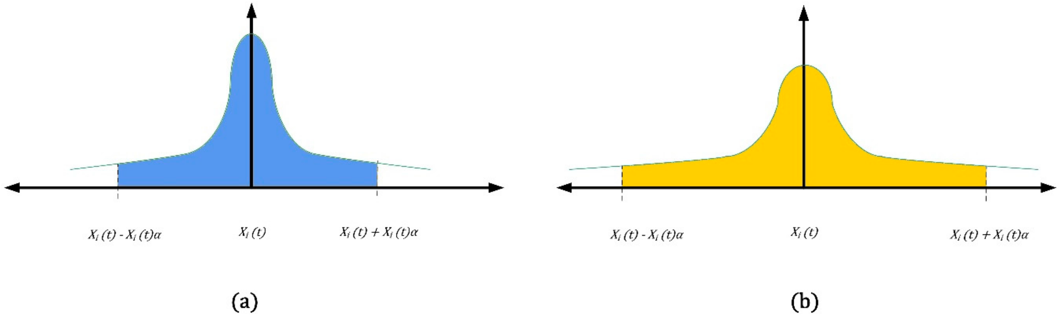
In light of these considerations, we review, in Figure 8 (Figure 8a refers to “drone a” and Figure 8b refers to “drone b”), the previous confidence interval area considered for uncertainty in Figure 6:

Due to the good knowledge of the systems and subsystems of the military drone (hereafter referred to as “drone b”), we can have the basis for a much wider Gaussian, and conversely, the value of α.

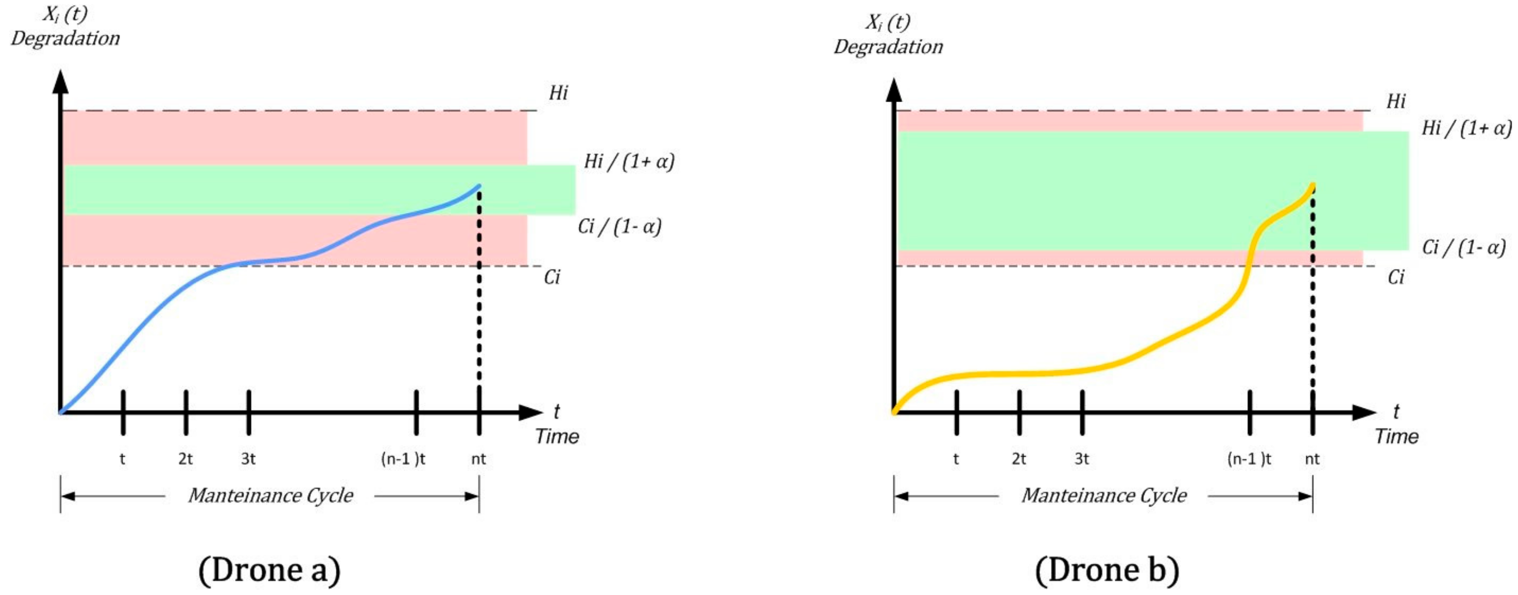
Reviewing the interval in Figure 7, for the two different drones we have the following uncertainties (see Figure 9):

Considering “Drone a”, although its reliability is considerably higher, the knowledge of the components is lower. All this is reflected, from the analytical point of view, in the “shrinking” of the green band (see Figure 9), or the limits of preventive and corrective maintenance which are very close to each other. From the real point of view, this means that if we do not want to overcome the new limit $H_i/\left(1+\alpha \right)$, it is necessary to slightly reduce interval t, with a consequent increase of maintenance costs and a decrease in the general figure of availability.

The “Drone b”, (military) has, despite a bit of “shearing” by the α factor dropping a good margin, an increase in the frequency of the maintenance cycle, which will always remain modest.

7. Conclusions

In this paper, the uncertainty in the choice of the preventive maintenance intervals with respect to the soft failure threshold have been investigated, taking into account the reliability and safety requirements for Unmanned Aerial Vehicles (UAV).

First, we examined the state of the art of the philosophy of the UAVs and the roles and capabilities of operators. However, the increase of their use is strongly accompanied by higher failure rates compared to conventional, manned airplanes.

Then, we correlated the reliability of the drones with the maintenance intervals: a higher failure rate leads to very expensive repairs. In order to improve safety, the duplication of the troublesome elements is not the only solution. Therefore, it is necessary to obtain the required reliability level by also using high-quality, derated components, combined with a very detailed selection of a redundant subsystem during the design phase.

The innovation of our paper passes first through the review of the optimization of the probabilistic functions (under the conditions of a real case). Then, we find the optimal point of maintenance. It will be necessary to take into account a very large number of variables for all systems and subsystems in order to minimize uncertainty.

Finally, by evaluating uncertainty through the confidence interval, it is possible to accurately determine the maintenance intervals in order to not exceed the new soft failure limit, that takes into account the general knowledge of the systems and subsystems, and to remain always within the preventive maintenance limit time (and budget).

References

- Petritoli, E.; Leccese, F.; Ciani, L. Reliability Degradation, Preventive and Corrective Maintenance of UAV Systems. In Proceedings of the 2018 5th IEEE International Workshop on Metrology for AeroSpace (MetroAeroSpace), Rome, Italy, 20–22 June 2018; pp. 430–434. [Google Scholar] [CrossRef]
- Hobbs, A.; Herwitz, S. Human Challenges in the Maintenance of Unmanned Aircraft Systems; Interim Report to FAA and NASA; NASA: Moffett Field, CA, USA, May 2006.
- Overview of Military Drones Used By the UK Armed Forces; House of Commons Library: London, UK, 2015.
- Bhamidipati, K.K.; Uhlig, D.; Neogi, N. Engineering Safety and Reliability into UAV Systems: Mitigating the Ground Impact Hazard; University of Illinois, Urbana-Champaign: Urbana, IL, USA, August 2007; Volume 61822. [Google Scholar] [CrossRef]
- Austin, R. Unmanned Aircraft Systems; Wiley: Hoboken, NJ, USA, May 2010; ISBN 978-0-470-05819-0. [Google Scholar]
- US Department of Defence. Electronic Reliability Design Handbook; Technical Report, MIL-HDBK-338B; US Department of Defence: Washington, DC, USA, 1998.
- Miller, J.A.; Minear, P.D.; Niessner, A.F.; DeLullo, A.M.; Geiger, B.R.; Long, L.N.; Horn, J.F. Intelligent Unmanned Air Vehicle Flight Systems. In Proceedings of the AIAA 2005-7081 Infotech@Aerospace Conference, Arlington, VA, USA, 3–5 September 2005. [Google Scholar]
- Schmidt, J.; Parker, R. Development of A UAV Mishap Human Factors Database. In Proceedings of the Unmanned Systems 1995 Proceedings, Washington, DC, USA, 10–12 July 1995. [Google Scholar]
- Ballenger, K. Unmanned Aircraft Systems—General Overview. In Proceedings of the Presented to American Institute of Aeronautics and Astronautics, San Diego, CA, USA, 26–28 March 2013. [Google Scholar]
- Paggi, R.; Mariotti, G.L.; Paggi, A.; Leccese, F. Optimization of Availability Operation via simulated Prognostics. In Proceedings of the Metrology for Aerospace, 2nd IEEE International Workshop, Benevento, Italy, 4–5 June 2015; pp. 44–48, ISBN 978-1-4799-7568-6. [Google Scholar] [CrossRef]
- Clough, B.T. Unmanned Aerial Vehicles: Autonomous Control Challenges, A Researcher’s Perspective. J. Aerosp. Comput. Inf. Commun. 2005, 2, 327–347. [Google Scholar] [CrossRef]
- Department of Defense. MIL-HDBK-217/F2 Reliability Prediction of Electronic Equipment; Department of Defense: Washington, DC, USA, 1995.
- De Francesco, E.; De Francesco, R. The CoDeF structure: A way to evaluate Ai including failures caused by multiple minor degradations. In Proceedings of the 2nd IEEE International Workshop Metrology for Aerospace, Benevento, Italy, 3–5 June 2015. [Google Scholar]
- Weibel, R.; Hansman, R.J. Safety Considerations for Operation of Different Classes of UAVs in the NAS. In Proceedings of the AIAA 3rd “Unmanned Unlimited” Technical Conference, Workshop and Exhibit, Infotech@Aerospace Conferences, Chicago, IL, USA, 20–23 September 2004. [Google Scholar] [CrossRef]
- Peroni, M.; Dolce, F.; Kingston, J.; Palla, C.; Fanfani, A.; Leccese, F. Reliability study for LEO satellites to assist the selection of end of life disposal methods. In Proceedings of the 3rd IEEE International Workshop on Metrology for Aerospace, MetroAeroSpace 2016—Proceedings, Florence, Italy, 21–23 June 2016; pp. 141–145. [Google Scholar]
- Kabir, A.; Bailey, C.; Lu, H.; Stoyanov, S. A review of data-driven prognostics in power electronics. In Proceedings of the 35th International Spring Seminar on Electronics Technology, Bad Aussee, Austria, 9–13 May 2012; pp. 189–192. [Google Scholar] [CrossRef]
- Heywood, J.B.; Sher, E. The Two-Stroke Cycle Engine: Its Development, Operation, and Design; Society of Automotive Engineers, Inc.: Warrendale, PA, USA, 1999. [Google Scholar]
- USAF Judge Advocate General’s Corps. USAF Accident Investigation Board Reports. Available online: http://usaf.aib.law.af.mil/ (accessed on 1 July 2008).
- US Department of Defense. Reliability Prediction of Electronic Components; Technical Report, MIL-HDBK-217/F2; Department of Defense: Washington, DC, USA, 1991.
- Smith, G.; Schroeder, J.B.; Navarro, S.; Haldeman, D. Development of a prognostics and health management capability for the Joint Strike Fighter. In Proceedings of the 1997 IEEE Autotestcon Proceedings AUTOTESTCON ‘97, IEEE Systems Readiness Technology Conference. Systems Readiness Supporting Global Needs and Awareness in the 21st Century, Anaheim, CA, USA, 22–25 September 1997; pp. 676–682. [Google Scholar] [CrossRef]
- Murtha, J.F. An Evidence Theoretical Approach to Design of Reliable Low-Cost UAV’s. Master’s Thesis, Virginia Polytechnic Institute and State University, Blacksburg, VA, USA, 2009. [Google Scholar]
- Liu, H.; Yu, J.; Zhang, P.; Li, S. A review on fault prognostics in integrated health management. In Proceedings of the 2009 9th International Conference on Electronic Measurement & Instruments, Beijing, China, 16–19 August 2009; pp. 267–270. [Google Scholar] [CrossRef]
- Beard, R.W.; McLain, T.W. Small Unmanned Aircraft—Theory and Practice; Princeton University Press: Princeton, NJ, USA, 2012. [Google Scholar]
- Ng, Y.; Tomblin, J.; Freisthler, M. NCAMP Standard Operating Procedures. Available online: https://www.niar.wichita.edu/coe/ncamp_documents/ncampsop/NSP%20100%20NCAMP%20Standard%20Operating%20Procedure%20March%2011% (accessed on 1 May 2012).
- Paggi, R.; Mariotti, G.L.; Paggi, A.; Calogero, A.; Leccese, F. Prognostics via physics-based probabilistic simulation approaches. In Proceedings of the 3rd IEEE International Workshop on Metrology for Aerospace, MetroAeroSpace 2016, Florence, Italy, 22–23 June 2016; pp. 130–135. [Google Scholar]
- De Oliveira Martins Franco, B.J.; Sandoval Góes, L.C. Failure Analysis Methods in Unmanned Aerial Vehicle (UAV) Applications. In Proceedings of the Proceedings of COBEM 2007 19th International Congress of Mechanical Engineering, Brasília, Brazil, 5–9 November 2007. [Google Scholar]
- Schirripa Spagnolo, G.; Papalillo, D.; Leccese, F. Forensic Metrology: Uncertainty of Measurements in Forensic Analysis. In Proceedings of the 20th IMEKO TC-4 International Symposium Measurement of Electrical Quantities, Benevento, Italy, 15–17 September 2014. [Google Scholar]
- De Francesco, E.; De Francesco, R.; Leccese, F.; Cagnetti, M. Risk analysis in aviation: The forensic point of view. In Proceedings of the 20th IMEKO TC4 Symposium on Measurements of Electrical Quantities, Research on Electrical and Electronic Measurement for the Economic Upturn, together with 18th TC4 International Workshop on ADC and DCA Modeling and Testing, Benevento, Italy, 15–17 September 2014; pp. 563–568. [Google Scholar]
- Caciotta, M.; Cerqua, V.; Leccese, F.; Giarnetti, S.; DeFrancesco, E.; De Francesco, E.; Scaldarella, N. A First Study on Prognostic System for Electric Engines Based on Envelope Analysis. In Proceedings of the IEEE International Workshop on Metrology for Aerospace, Benevento, Italy, 29–30 May 2014. [Google Scholar]
- Blom, J.D. Unmanned Aerial System a Historical Perspective; Combat Studies Institute Press: Fort Leavenwort, KS, USA, 2010; Available online: https://usacac.army.mil/cac2/cgsc/carl/download/csipubs/OP37.pdf (accessed on 5 April 2018).
- ASD/AIA. S3000L International Procedure Specification for Logistic Support Analysis LSA. Issue 1.1. 24 July 2014. Available online: http://www.s3000l.org/ (accessed on 9 May 2016).
- Kakaes, K.; Greenwood, F.; Lippincott, M.; Dosemagen, S.; Meier, P.; Wich, S. Drones and Aerial Observation: New Technologies for Property Rights, Human Rights, and Global Development. New America. 2015. Available online: http://www.rhinoresourcecenter.com/pdf_files/143/1438073140.pdf (accessed on 5 May 2016).
- De Angelis, G.; Dati, E.; Bernabei, M.; Leccese, F. Development on aerospace composite structures investigation using thermography and shearography in comparison to traditional NDT methods. In Proceedings of the 2nd IEEE International Workshop on Metrology for Aerospace, MetroAeroSpace 2015, Benevento, Italy, 4–5 June 2015; pp. 49–55. [Google Scholar] [CrossRef]
- Draper, M.; Calhoun, G.; Ruff, H.; Williamson, D.; Barry, T. Manual versus Speech Input for the Unmanned Aerial Vehicle Control Station Operations. In Proceedings of the 47th Annual Meeting Human Factors and Ergonomics Society, Denver, CO, USA, 13–17 October 2003. [Google Scholar]
- Tobon-Mejia, D.A.; Medjaher, K.; Zerhouni, N.; Tripot, G. A Data-Driven Failure Prognostics Method Based on Mixture of Gaussians Hidden Markov Models. IEEE Trans. Reliab. 2012, 61, 491–503. [Google Scholar] [CrossRef] [Green Version]
- Reimann, S.; Amos, J.; Bergquist, E.; Cole, J.; Phillips, J.; Shuster, S. UAV for Reliability Build; Technical Report; Department of Aerospace Engineering and Mechanics, University of Minnesota: Minneapolis, MN, USA, May 2014. [Google Scholar]
- Bianchi, S.; Paggi, R.; Mariotti, G.L.; Leccese, F. Why and When Must the Preventive Maintenance be Performed? In Proceedings of the IEEE International Workshop on Metrology for Aerospace, Benevento, Italy, 29–30 May 2014; pp. 221–226. [Google Scholar]
- USA Department of Defense. MIL-1388-2B Logistics Support Analysis Record. Available online: http://ld.hq.nasa.gov/docs/MILSTD-1388-2B_DoD_Requirements.pdf (accessed on 5 May 2016).
- Wichita State University; SAE International. Polymer Matrix Composites: Guidelines for Characterization of Structural Materials; ASTM International: West Conshohocken, PA, USA, 2002; Volume 1, ISBN 978-0-7680-7811-4. [Google Scholar]
- Saha, B.; Goebel, K.; Christophersen, J. Comparison of prognostic algorithms for estimating remaining useful life of batteries. Trans. Inst. Meas. Control SAGE J. 2009, 31, 293–308. Available online: http://tim.sagepub.com/content/31/3-4/293.abstract (accessed on 5 May 2016). [CrossRef] [Green Version]
- Wood, S. Autonomous Underwater Gliders. In Underwater Vehicles; Inzartsev, A.V., Ed.; In-Tech: Vienna, Austria, 2009; Chapter 26; pp. 499–524. [Google Scholar]
- Kayton, M.; Fried, W.R. Avionics Navigation Systems; Wiley: Hoboken, NJ, USA, 1997. [CrossRef]
- Wang, T.; Yu, J.; Siegel, D.; Lee, J. A similarity-based prognostics approach for Remaining Useful Life estimation of engineered systems. In Proceedings of the International Conference on Prognostics and Health Management, Denver, CO, USA, 6–9 October 2008; pp. 1–6. [Google Scholar] [CrossRef]
- Schaefer, R. Unmanned Aerial Vehicle Reliability Study; Office of the Secretary of Defense: Washington, DC, USA, February 2003. [Google Scholar]
- Zio, E.; Di Maio, F. A data-driven fuzzy approach for predicting the remaining useful life in dynamic failure scenarios of a nuclear system. Reliab. Eng. Syst. Saf. 2010, 95, 49–57. [Google Scholar] [CrossRef] [Green Version]
- Petritoli, E.; Leccese, F.; Ciani, L. Reliability assessment of UAV systems. In Proceedings of the 2017 IEEE International Workshop on Metrology for AeroSpace (MetroAeroSpace), Padua, Italy, 21–23 June 2017; pp. 266–270. [Google Scholar] [CrossRef]
- Gnedenko, B.; Belyayev, Y.; Solovyev, A.D. Mathematical Methods of Reliability Theory; Barlow, R.E., Ed.; Academic Press: New York, NY, USA, 1969. [Google Scholar]
- Lloyd, D.; Lipow, M. Reliability: Management, Methods, and Mathematics. Am. Math. Mon. 1963, 70, 342. [Google Scholar]
- Romig, H. Binomial Table; John Wiley and Sons, Inc.: New York, NY, USA, 1953. [Google Scholar]
- Shooman, M. Probabilistic Reliability: An Engineering Approach; McGraw-Hill: New York, NY, USA, 1968. [Google Scholar]
- Rao, C. Linear Statistical Inference and Its Applications; John Wiley and Sons, Inc.: New York, NY, USA, 1977. [Google Scholar]
- Mann, N.; Schafer, R.; Sigpurwalla, N. Mathematical Methods for Statistical Analysis of Reliability and Life Data; John Wiley and Sons, Inc.: New York, NY, USA, 1974. [Google Scholar]
- Graver, J.G.; Liu, J.; Woolsey, C.; Leonard, N.E. Design and Analysis of an Underwater Vehicle for Controlled Gliding. In Proceedings of the 1998 Conference on Information Sciences and Systems, Princeton, NJ, USA, 15–17 March 1998; pp. 801–806. [Google Scholar]
- Chen, Y.; Chen, T. Implementing Fault-Tolerance via Modular Redundancy with Comparison. IEEE Trans. Reliab. 1990, 39, 217–225. [Google Scholar] [CrossRef]
- Feldstein, C.B.; Muzio, J.C. Development of a Fault Tolerant Flight Control System. In Proceedings of the 23rd Digital Avionics Systems Conference (IEEE Cat. No. 04CH37576), Salt Lake City, UT, USA, 28 October 2004; p. 6.E.3-61. [Google Scholar] [CrossRef]
- Khan, R.; Williams, P.; Riseborough, P.; Rao, A.; Hill, R. Active Fault Tolerant Flight Control System Design—A UAV Case Study. Available online: https://arxiv.org/abs/1610.03162v1 (accessed on 7 May 2016).
- Ducard, G.J.J. Fault-tolerant Flight Control and Guidance Systems. In Practical Methods for Small Unmanned Aerial Vehicles; Springer: Berlin, Germany, 2009; Volume XXII, p. 264. [Google Scholar]
- Kobayashi, Y.; Takahashi, M. Design of Intelligent Fault-Tolerant Flight Control System for Unmanned Aerial Vehicles. Keio University. Japan. Nihon Kikai Gakkai Ronbunshu C Hen/Trans. Jpn. Soc Mech Eng. Part C 2009, 75, 2301–2310. [Google Scholar]
- Zhang, X.; Li, H.; Yuan, D. Dual Redundant Flight Control System Design for Microminiature. UAV. In Proceedings of the 2nd International Conference on Electrical, Computer Engineering and Electronics, Jinan, China, 29–31 May 2015. [Google Scholar] [CrossRef]
- Department of the Army. Reliability/Availability of Electrical and Mechanical Systems for Command, Control, Communications, Computer, Intelligence, Surveillance and Reconnaissance (C4ISR) Facilities. TM 5-698-1. 2003. Available online: https://www.wbdg.org/FFC/ARMYCOE/COETM/tm_5_698_1.pdf (accessed on 1 March 2018).
- Poole, J. A Fast Reliability Analysis for an Unmanned Aerial Vehicle Performing a Phased Mission. Ph.D. Thesis, Loughborough University, Loughborough, UK, 2011. Available online: https://dspace.lboro.ac.uk/2134/8775 (accessed on 1 March 2018).
- Zhu, Q. Maintenance Optimization for Multi-Component Systems under Condition Monitoring. Technische Universiteit Eindhoven, Eindhoven. 2015. Available online: https://pure.tue.nl/ws/portalfiles/portal/3934830/784814.pdf (accessed on 1 March 2018).
- Zhu, Q.; Peng, H.; van Houtum, G.J. A condition-based maintenance policy for multicomponent systems with a high maintenance setup cost. In OR Spectrum; Springer: Berlin, Germany, 2015; Volume 37, pp. 1007–1035. [Google Scholar] [CrossRef]
- DSIAC. Reliability of UAVs and Drones. Available online: https://www.dsiac.org/resources/journals/dsiac/spring-2017-volume-4-number-2/reliability-uavs-and-drones (accessed on 1 March 2018).
Figure 1.
Failure Rate vs. Flight hours for the F-16 and some common drones (figure extrapolated on the data of: Barnard Microsystems Inc. et al. [5]).
Figure 2.
The Hierarchy of the Reliability Assessment (every 103 system failures) for UAVs. The structure is subdivided into main systems (yellow), subsystems (blue), all together representing the UAV system (orange); (figure extrapolated on the data of: Barnard Microsystems Inc. et al. [5]).
Figure 3.
Degradation threshold of a system with a cycle of corrective maintenance only.
Figure 4.
(a) Maintenance limit of preventive maintenance; (b) maintenance limit corrective maintenance.
Figure 5.
Uncertainty evaluation of corrective maintenance: the inspection point at 3t in detailed and expanded as a confidence interval.
Figure 6.
Confidence interval area considered for uncertainty.
Figure 7.
Uncertainty evaluation of corrective maintenance: original interval area (red) and the evaluation of the confidence interval (green).
Figure 8.
Confidence interval area considered for uncertainty: commercial drone (blue) and military (yellow).
Figure 9.