Phenoliner: A New Field Phenotyping Platform for Grapevine Research

 , and
, and
Abstract
:1. Introduction
2. Materials and Methods
2.1. Plant Material
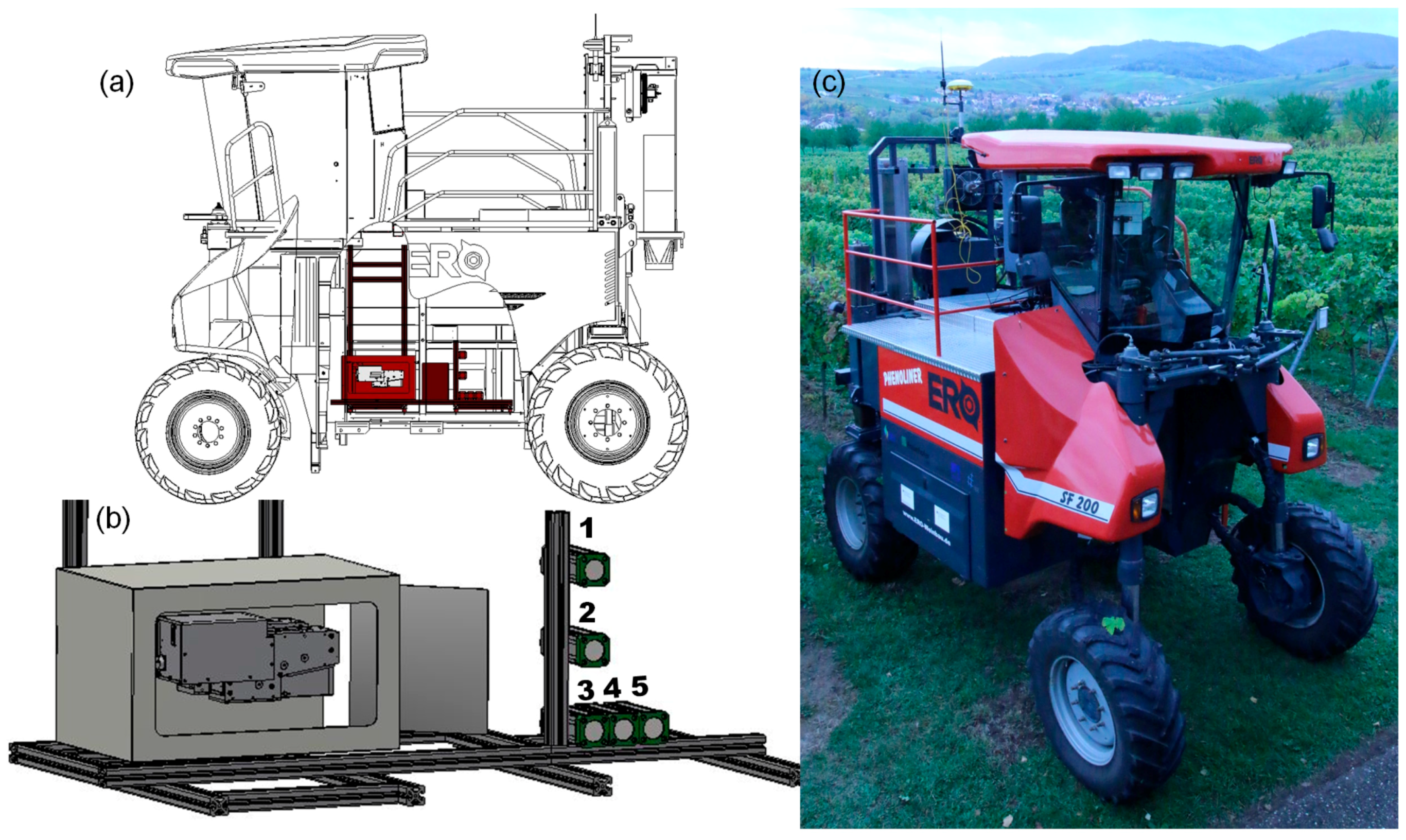
2.2. Vehicle
- In order to standardise the light conditions within the tunnel the base frame on the right hand side of the vehicle was extended and covered with metal plates. All slots in between were sealed and a curtain was installed in the back of the tunnel to avoid direct sun light interference
- Due to safety reasons on top of the machine the railing was enlarged where parts of the harvesting machine had been removed.
- The energy necessary for sensors, light units, and computer is provided by a generator driven by the vehicle. Two operating modes are possible: (1) diesel engine on and (2) diesel engine off. Due to the removal of the original harvesting hydraulics the free energy of the diesel engine can be used for powering a generator when the engine is on. Furthermore, it is possible to connect the vehicle to a regular power socket (230 V) when the engine is off. Two backup batteries (minimum 0.5 kWh) are bridging the time between turning off the engine and connecting the vehicle to the socket. This solution permits the transfer of the acquired data from the computers on the vehicle to the memory location without having the engine run for hours. There are 20 sockets available on the vehicle (cab: 2; front part: 9; back part: 9), provided with a suitable fuse through a distribution box.
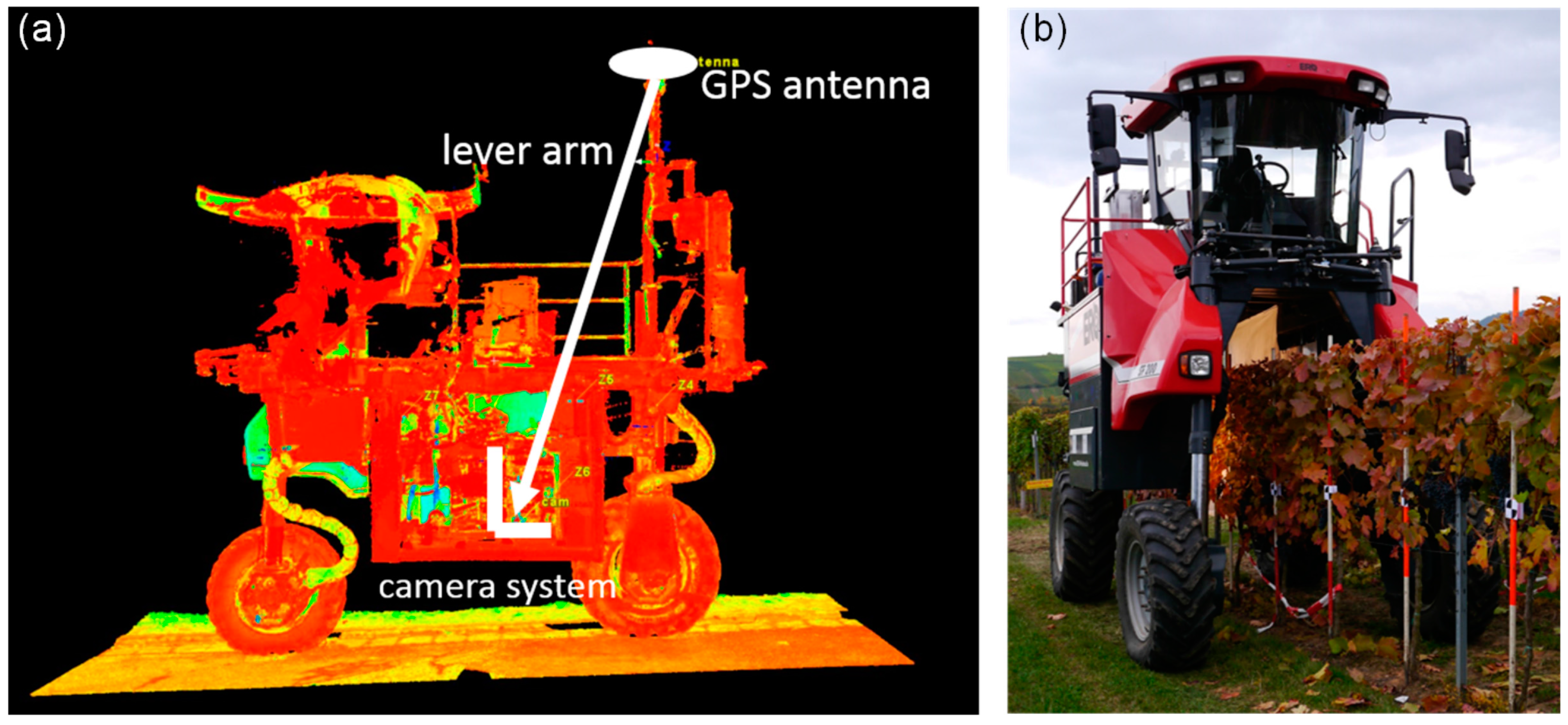
2.3. RTK-GPS
2.4. SensorA: Multicamerasystem (RGB, NIR)
2.5. Sensor B: Hyperspectral Camera System
3. Application of the Phenoliner: Pilot Study
3.1. Sensor A
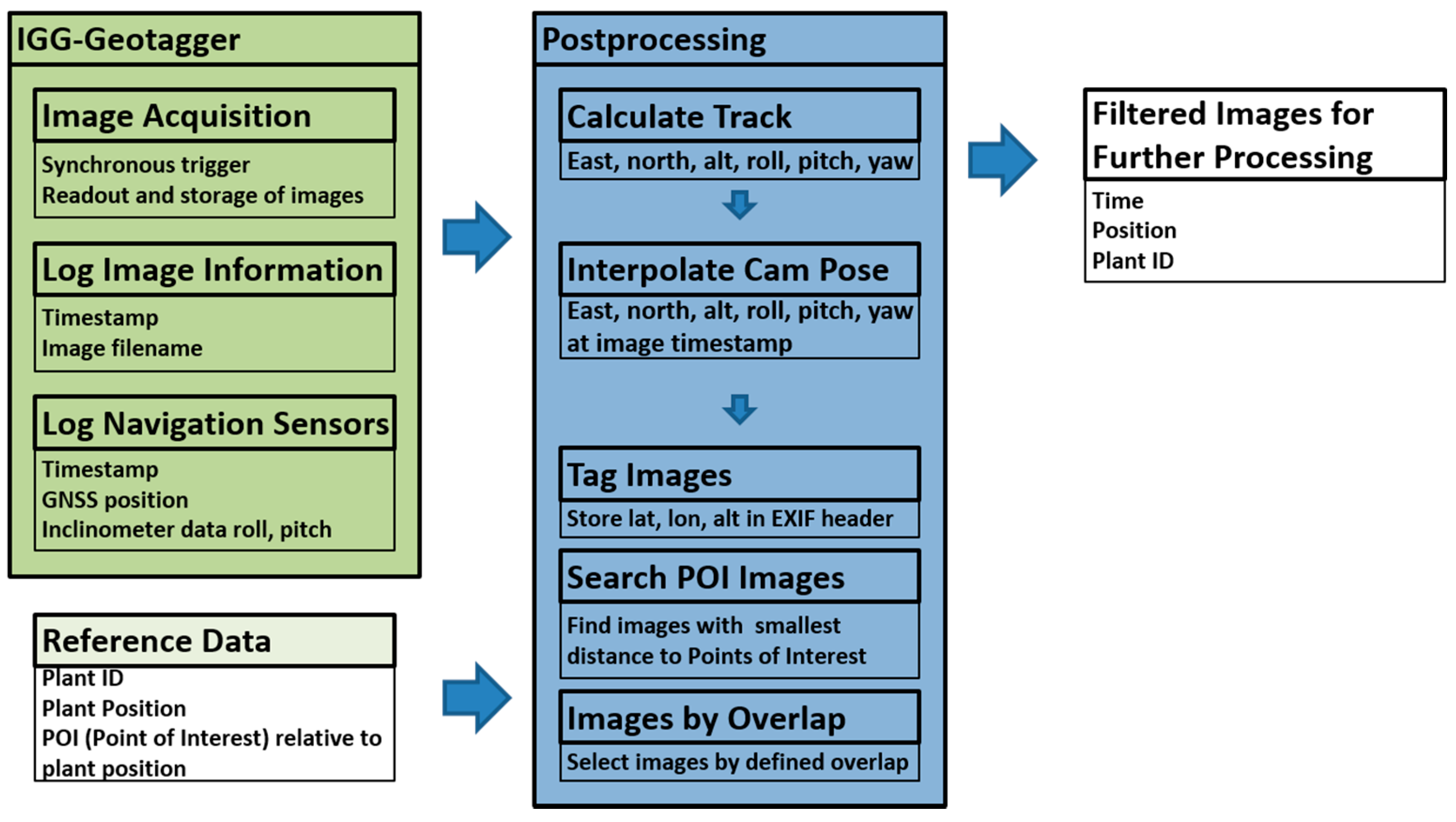
3.1.1. IGG Geotagger 2.0: Geo-Referencing of Images
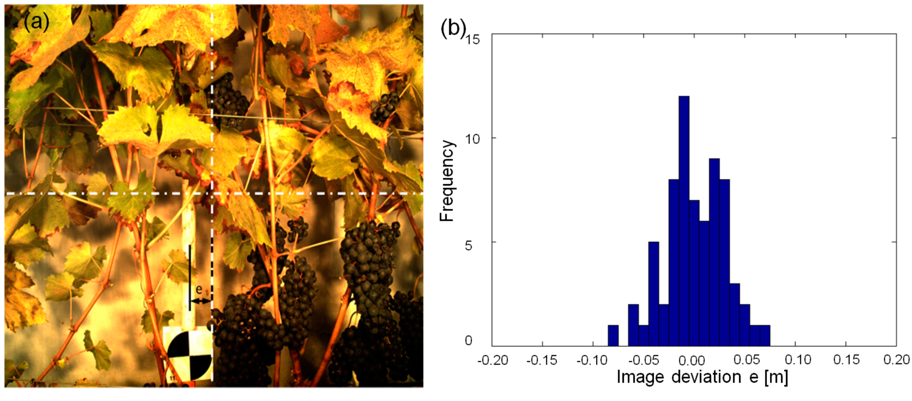
3.1.2. Validation
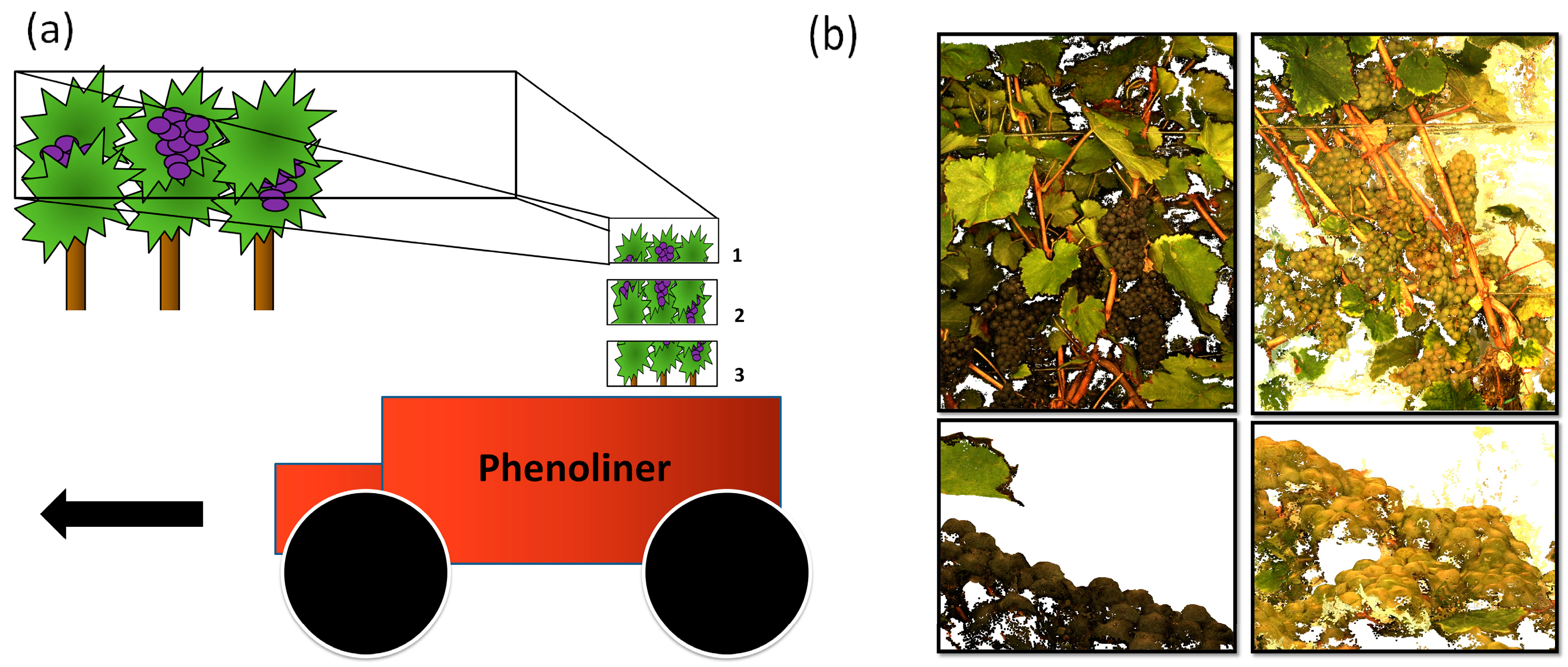
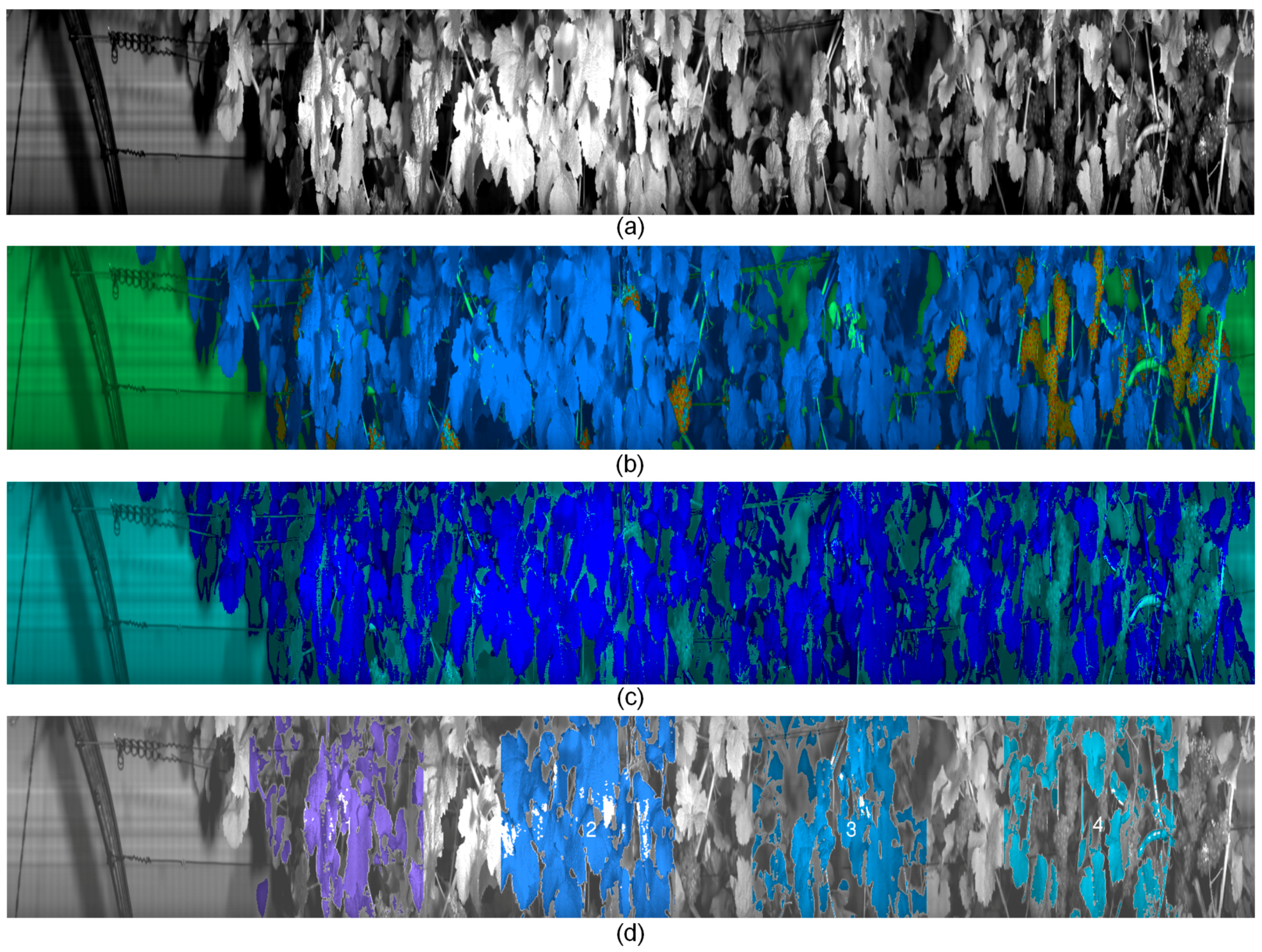
3.1.3. Application Example: 3D Reconstruction of the Full Vine Row
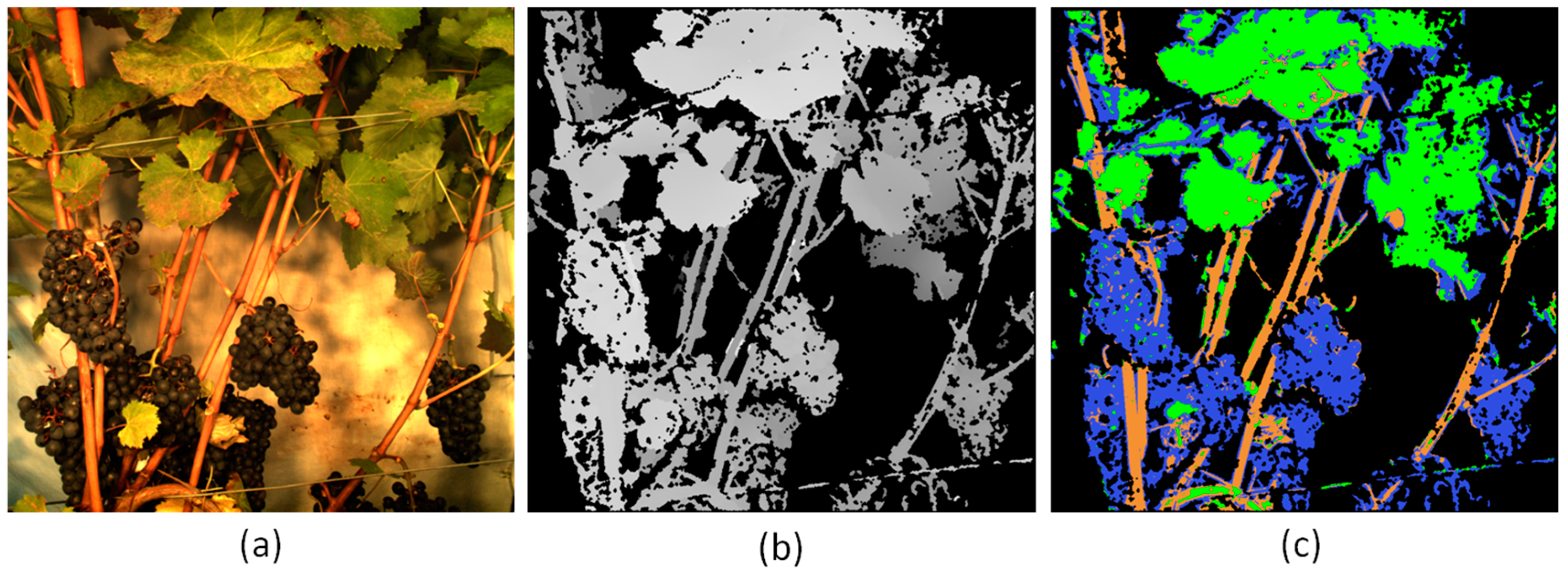
3.1.4. Application Example: Depth Map Creation and Segmentation of Single Vines
3.2. Sensor B
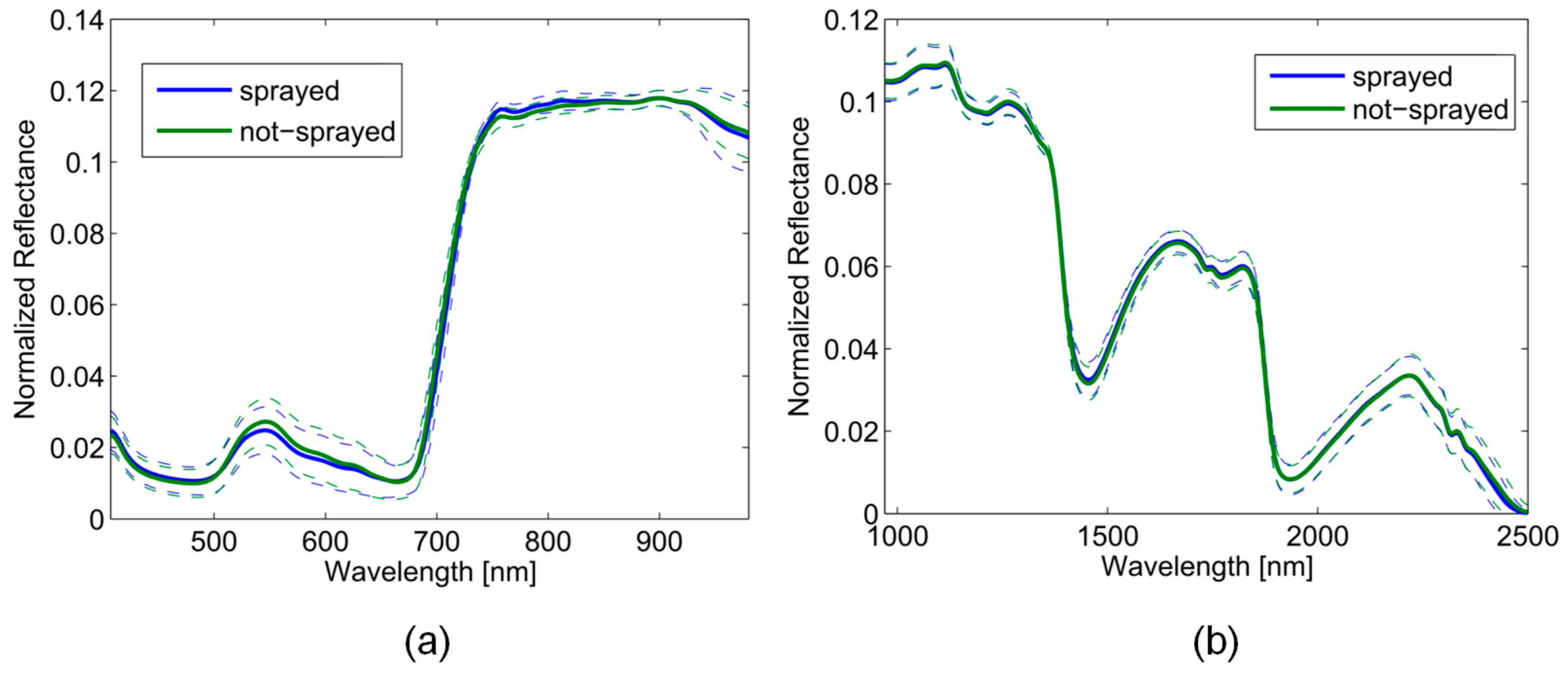
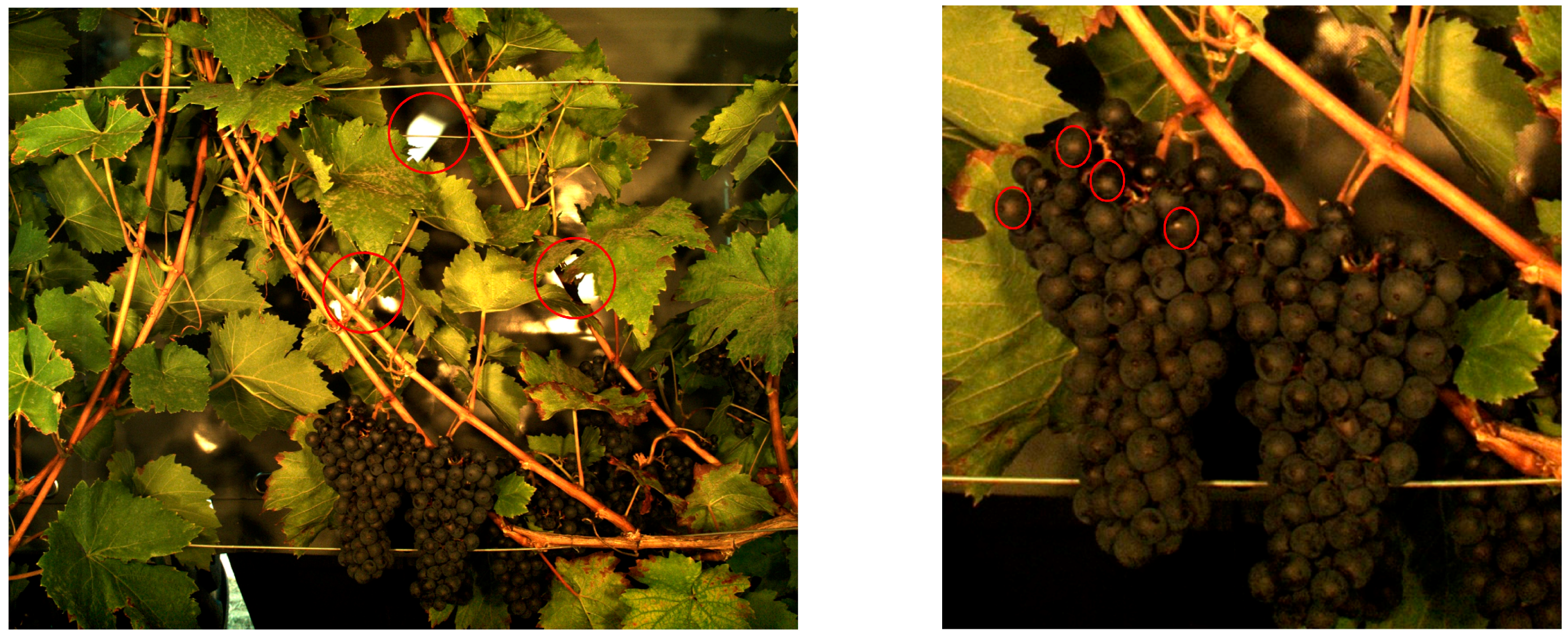
3.2.1. Hyperspectral Image Acquisition
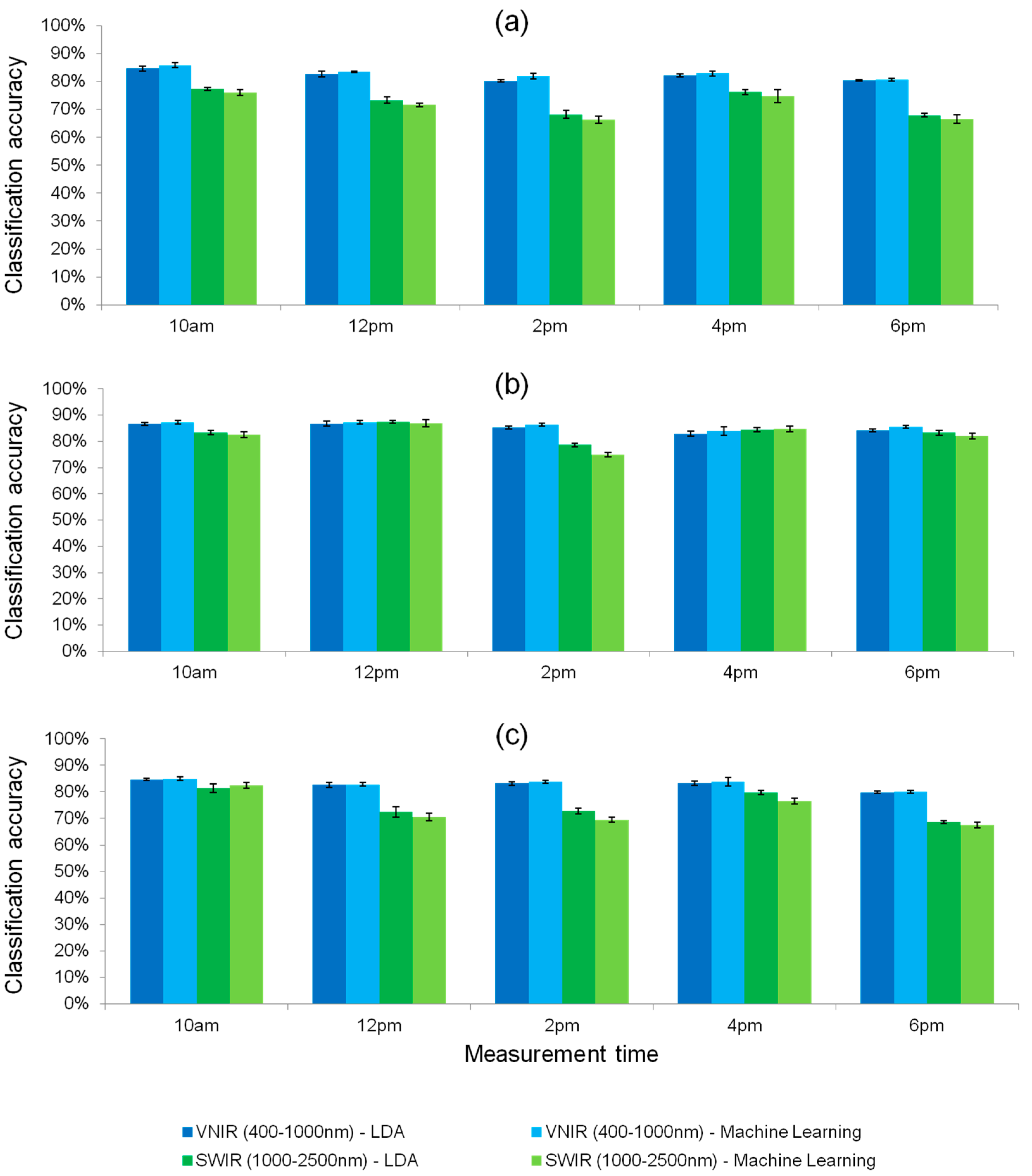
3.2.2. Validation
3.3. Discussion of One Year Experiences with the Phenoliner
3.3.1. Sensor A
3.3.2. Sensor B
4. Conclusions
Acknowledgments
Author Contributions
Conflicts of Interest
References
- Granier, C.; Aguirrezabal, L.; Chenu, K.; Cookson, S.J.; Dauzat, M.; Hamard, P.; Thioux, J.J.; Rolland, G.; Bouchier-Combaud, S.; Lebaudy, A.; et al. Phenopsis, an automated platform for reproducible phenotyping of plant responses to soil water deficit in arabidopsis thaliana permitted the identification of an accession with low sensitivity to soil water deficit. New Phytol. 2006, 169, 623–635. [Google Scholar] [CrossRef] [PubMed]
- Walter, A.; Scharr, H.; Gilmer, F.; Zierer, R.; Nagel, K.A.; Ernst, M.; Wiese, A.; Virnich, O.; Christ, M.M.; Uhlig, B.; et al. Dynamics of seedling growth acclimation towards altered light conditions can be quantified via growscreen: A setup and procedure designed for rapid optical phenotyping of different plant species. New Phytol. 2007, 174, 447–455. [Google Scholar] [CrossRef] [PubMed]
- Hartmann, A.; Czauderna, T.; Hoffmann, R.; Stein, N.; Schreiber, F. Htpheno: An image analysis pipeline for high-throughput plant phenotyping. BMC Bioinform. 2011. [Google Scholar] [CrossRef] [PubMed]
- Reuzeau, C.; Frankard, V.; Hatzfeld, Y.; Sanz, A.; Van Camp, W.; Lejeune, P.; De Wilde, C.; Lievens, K.; De Wolf, J.; Vranken, E.; et al. Traitmill™: A functional genomics platform for the phenotypic analysis of cereals. Plant Genet. Resources 2006, 4, 20–24. [Google Scholar] [CrossRef]
- Lejealle, S.; Bailly, G.; Masdoumier, G.; Ayral, J.L.; Latouche, G.; Cerovic, Z. Pre-symptomatic detection of downy mildew using multiplex-330®. In Proceedings of the 10e Conférence Internationale sur les Maladies des Plantes, Tours, France, 3–5 December 2012; pp. 63–73. [Google Scholar]
- Latouche, G.; Debord, C.; Raynal, M.; Milhade, C.; Cerovic, Z.G. First detection of the presence of naturally occurring grapevine downy mildew in the field by a fluorescence-based method. Photochem. Photobiol. Sci. 2015, 14, 1807–1813. [Google Scholar] [CrossRef] [PubMed]
- Agati, G.; D'Onofrio, C.; Ducci, E.; Cuzzola, A.; Remorini, D.; Tuccio, L.; Lazzini, F.; Mattii, G. Potential of a multiparametric optical sensor for determining in situ the maturity components of red and white vitis vinifera wine grapes. J. Agric. Food Chem. 2013, 61, 12211–12218. [Google Scholar] [CrossRef] [PubMed]
- Ghozlen, N.B.; Cerovic, Z.G.; Germain, C.; Toutain, S.; Latouche, G. Non-destructive optical monitoring of grape maturation by proximal sensing. Sensors 2010, 10, 10040. [Google Scholar] [CrossRef] [PubMed]
- Diago, M.P.; Sanz-Garcia, A.; Millan, B.; Blasco, J.; Tardaguila, J. Assessment of flower number per inflorescence in grapevine by image analysis under field conditions. J. Sci. Food Agric. 2014, 94, 1981–1987. [Google Scholar] [CrossRef] [PubMed]
- Grossetete, M.; Berthoumieu, Y.; Da Costa, J.P.; Germain, C.; Lavialle, O.; Grenier, G. Early estimation of vineyard yield: Site specific counting of berries by using a smartphone. In Proceedings of the International Conference of Agricultural Engineering on Infomation Technology, Automation and Precision Farming, Valencia, Spain, 8–12 July 2012. [Google Scholar]
- Rabatel, G.; Guizard, C. Grape berry calibration by computer vision using elliptical model fitting. In Proceedings of the 6th European Conference on Precision Agriculture ECPA, Skiathos, Greece, 3–6 June 2007; pp. 581–587. [Google Scholar]
- Johnson, L.F.; Roczen, D.E.; Youkhana, S.K.; Nemani, R.R.; Bosch, D.F. Mapping vineyard leaf area with multispectral satellite imagery. Comput. Electron. Agric. 2003, 38, 33–44. [Google Scholar] [CrossRef]
- Losos, J.; Arnold, S.; Bejerano, G.; Brodie, E.I.; Hibbett, D. Evolutionary biology for the 21st century. PLoS Biol. 2013, 11, e1001466. [Google Scholar] [CrossRef] [PubMed]
- Bellvert, J.; Zarco-Tejada, P.J.; Girona, J.; Fereres, E. Mapping crop water stress index in a ‘pinot-noir’ vineyard: Comparing ground measurements with thermal remote sensing imagery from an unmanned aerial vehicle. Precis. Agric. 2014, 15, 361–376. [Google Scholar] [CrossRef]
- Mazzetto, F.; Calcante, A.; Mena, A.; Vercesi, A. Integration of optical and analogue sensors for monitoring canopy health and vigour in precision viticulture. Precis. Agric. 2010, 11, 636–649. [Google Scholar] [CrossRef]
- Bourgeon, M.-A.; Paoli, J.-N.; Jones, G.; Villette, S.; Gée, C. Field radiometric calibration of a multispectral on-the-go sensor dedicated to the characterization of vineyard foliage. Comput. Electron. Agric. 2016, 123, 184–194. [Google Scholar] [CrossRef]
- Bramley, R.G.V.; Trought, M.C.T.; Praat, J.P. Vineyard variability in marlborough, new zealand: Characterising variation in vineyard performance and options for the implementation of precision viticulture. Aust. J. Grape Wine Res. 2011, 17, 72–78. [Google Scholar] [CrossRef]
- Bramley, R.; Kleinlagel, B.; Ouzman, J. A Protocol for the Construction of Yield Maps from Data Collected Using Commercially Available Grape Yield Monitors—Supplement No. 2. April 2008—Accounting for ‘Convolution’ in Grape Yield Mapping. Available online: http://www.cse.csiro.au/client_serv/resources/protocol_supp2.pdf (accessed on 10 January 2017).
- Llorens, J.; Gil, E.; Llop, J.; Queralto, M. Georeferenced lidar 3d vine plantation map generation. Sensors 2011, 11, 6237–6256. [Google Scholar] [CrossRef] [PubMed]
- Arnó, J.; Escolà, A.; Vallès, J.; Llorens, J.; Sanz, R.; Masip, J.; Palacín, J.; Rosell-Polo, J. Leaf area index estimation in vineyards using a ground-based lidar scanner. Precis. Agric. 2013, 14, 290–306. [Google Scholar] [CrossRef]
- Nuske, S.; Wilshusen, K.; Achar, S.; Yoder, L.; Narasimhan, S.; Singh, S. Automated visual yield estimation in vineyards. J. Field Robot. 2014, 31, 837–860. [Google Scholar] [CrossRef]
- Araus, J.L.; Cairns, J.E. Field high-throughput phenotyping: The new crop breeding frontier. Trends Plant. Sci. 2014, 19, 52–61. [Google Scholar] [CrossRef] [PubMed]
- Matese, A.; Di Gennaro, S. Technology in precision viticulture: A state of the art review. Int. J. Wine Res. 2015, 7, 69–81. [Google Scholar] [CrossRef]
- Vinerobot. Available online: http://www.vinerobot.eu/ (accessed on 1 February 2017).
- Robotnik Vinbot Project—Robotnik. Available online: http://www.robotnik.eu/portfolio/robotnik-proyecto-vinbot/ (accessed on 1 February 2017).
- Wall-ye. Available online: http://www.wall-ye.com/ (accessed on 1 February 2017).
- Kicherer, A.; Herzog, K.; Pflanz, M.; Wieland, M.; Rüger, P.; Kecke, S.; Kuhlmann, H.; Töpfer, R. An automated phenotyping pipeline for application in grapevine research. Sensors 2015, 15, 4823–4836. [Google Scholar] [CrossRef] [PubMed]
- Vineguard. Available online: http://robotics.bgu.ac.il/index.php/Development_of_an_Autonomous_vineyard_sprayer (accessed on 1 February 2017).
- Vision Robotics Corporation. Available online: http://www.visionrobotics.com/vr-grapevine-pruner (accessed on 1 February 2017).
- Vitirover. Available online: http://www.vitirover.com/fr/ (accessed on 1 February 2017).
- Kicherer, A. High-Throughput Phenotyping of Yield Parameters for Modern Grapevine Breeding; University of Hohenheim, Julius Kühn-lnstitut, Federal Research Centre for Cultivated Plants: Quedlinburg, Germany, 2015. [Google Scholar]
- Kicherer, A.; Klodt, M.; Sharifzadeh, S.; Cremers, D.; Töpfer, R.; Herzog, K. Automatic image-based determination of pruning mass as a determinant for yield potential in grapevine management and breeding. Aust. J. Grape Wine Res. 2016. [Google Scholar] [CrossRef]
- Klodt, M.; Herzog, K.; Töpfer, R.; Cremers, D. Field phenotyping of grapevine growth using dense stereo reconstruction. BMC Bioinf. 2015. [Google Scholar] [CrossRef] [PubMed]
- Herzog, K.; Roscher, R.; Wieland, M.; Kicherer, A.; Läbe, T.; Förstner, W.; Kuhlmann, H.; Töpfer, R. Initial steps for high-throughput phenotyping in vineyards. Vitis 2014, 53, 1–8. [Google Scholar]
- Abraham, S.; Hau, T. Towards autonomous high-precision calibration of digital cameras. In Proceedings of the SPIE Annual Meeting, San Diego, CA, USA, 27 July 1997; pp. 82–93. [Google Scholar]
- Rose, J.; Kicherer, A.; Wieland, M.; Klingbeil, L.; Töpfer, R.; Kuhlmann, H. Towards automated large-scale 3d phenotyping of vineyards under field conditions. Sensors 2016, 16, 2136. [Google Scholar] [CrossRef] [PubMed]
- Roscher, R.; Herzog, K.; Kunkel, A.; Kicherer, A.; Töpfer, R.; Förstner, W. Automated image analysis framework for high-throughput determination of grapevine berry sizes using conditional random fields. Comput. Electron. Agric. 2014, 100, 148–158. [Google Scholar] [CrossRef]
- Furukawa, Y.; Ponce, J. Accurate, dense, and robust multiview stereopsis. IEEE Trans. Pattern Anal. Mach. Intell. 2010, 32, 1362–1376. [Google Scholar] [CrossRef] [PubMed]
- Martinetz, T.M.; Berkovich, S.G.; Schulten, K.J. ‘neural-gas’ network for vector quantization and its application to time-series prediction. IEEE Trans. Neural Netw. 1993, 4, 558–569. [Google Scholar] [CrossRef] [PubMed]
- Wold, S.; Sjöström, M.; Eriksson, L. Pls-regression: A basic tool of chemometrics. Chemometrics Intellig. Lab. Syst. 2001, 58, 109–130. [Google Scholar] [CrossRef]
- Moody, J.; Darken, C.J. Fast learning in networks of locally-tuned processing units. Neural Comput. 1989, 1, 281–294. [Google Scholar] [CrossRef]
- Cybenko, G. Approximation by superpositions of a sigmoidal function. Math. Control Signals Syst. (MCSS) 1989, 2, 303–314. [Google Scholar] [CrossRef]
- Bishop, C.M. Pattern Recognition and Machine Learning; Springer: New York, NY, USA, 2006; Volume 4, Chapter 4. [Google Scholar]


| VNIR | SWIR | |||||||||
|---|---|---|---|---|---|---|---|---|---|---|
| West and east canopy side | ||||||||||
| PNET | MLP | RBF | PLS | PNET | MLP | RBF | PLS | |||
| 10 a.m. | 81.80% | 79.40% | 86.85% | 86.55% | 10 a.m. | 70.95% | 70.25% | 77.65% | 77.80% | |
| 12 p.m. | 81.30% | 81.40% | 83.90% | 83.05% | 12 p.m. | 66.65% | 66.70% | 72.25% | 73.95% | |
| 2 p.m. | 77.05% | 77.65% | 83.40% | 80.95% | 2 p.m. | 60.30% | 59.90% | 67.95% | 69.25% | |
| 4 p.m. | 80.10% | 79.75% | 84.00% | 82.45% | 4 p.m. | 67.30% | 67.15% | 78.00% | 77.15% | |
| 6 p.m. | 78.75% | 78.95% | 81.30% | 81.80% | 6 p.m. | 63.25% | 64.45% | 69.10% | 68.40% | |
| West side | ||||||||||
| PNET | MLP | RBF | PLS | PNET | MLP | RBF | PLS | |||
| 10 a.m. | 81.25% | 83.05% | 87.95% | 87.65% | 10 a.m. | 73.35% | 72.05% | 84.60% | 83.95% | |
| 12 p.m. | 84.90% | 85.20% | 88.05% | 87.80% | 12 p.m. | 81.20% | 80.65% | 88.00% | 88.25% | |
| 2 p.m. | 79.50% | 80.70% | 87.05% | 85.60% | 2 p.m. | 68.55% | 71.45% | 75.30% | 77.50% | |
| 4 p.m. | 82.95% | 81.85% | 84.70% | 83.90% | 4 p.m. | 70.60% | 73.15% | 85.60% | 84.60% | |
| 6 p.m. | 83.65% | 82.15% | 86.30% | 85.80% | 6 p.m. | 72.45% | 72.20% | 83.95% | 84.10% | |
| East side | ||||||||||
| PNET | MLP | RBF | PLS | PNET | MLP | RBF | PLS | |||
| 10 a.m. | 80.25% | 82.05% | 85.60% | 85.15% | 10 a.m. | 76.20% | 73.45% | 83.85% | 83.50% | |
| 12 p.m. | 78.05% | 79.00% | 83.40% | 83.85% | 12 p.m. | 64.20% | 63.55% | 71.75% | 73.60% | |
| 2 p.m. | 80.35% | 78.55% | 84.55% | 83.45% | 2 p.m. | 64.90% | 64.85% | 70.45% | 73.90% | |
| 4 p.m. | 80.05% | 79.45% | 85.55% | 83.95% | 4 p.m. | 71.10% | 71.25% | 77.95% | 80.75% | |
| 6 p.m. | 77.65% | 76.70% | 80.45% | 80.15% | 6 p.m. | 63.55% | 63.50% | 68.90% | 69.50% | |
© 2017 by the authors. Licensee MDPI, Basel, Switzerland. This article is an open access article distributed under the terms and conditions of the Creative Commons Attribution (CC BY) license (http://creativecommons.org/licenses/by/4.0/).
Share and Cite
Kicherer, A.; Herzog, K.; Bendel, N.; Klück, H.-C.; Backhaus, A.; Wieland, M.; Rose, J.C.; Klingbeil, L.; Läbe, T.; Hohl, C.; et al. Phenoliner: A New Field Phenotyping Platform for Grapevine Research. Sensors 2017, 17, 1625. https://doi.org/10.3390/s17071625
Kicherer A, Herzog K, Bendel N, Klück H-C, Backhaus A, Wieland M, Rose JC, Klingbeil L, Läbe T, Hohl C, et al. Phenoliner: A New Field Phenotyping Platform for Grapevine Research. Sensors. 2017; 17(7):1625. https://doi.org/10.3390/s17071625
Chicago/Turabian StyleKicherer, Anna, Katja Herzog, Nele Bendel, Hans-Christian Klück, Andreas Backhaus, Markus Wieland, Johann Christian Rose, Lasse Klingbeil, Thomas Läbe, Christian Hohl, and et al. 2017. "Phenoliner: A New Field Phenotyping Platform for Grapevine Research" Sensors 17, no. 7: 1625. https://doi.org/10.3390/s17071625