Soil Moisture Content Estimation Based on Sentinel-1 and Auxiliary Earth Observation Products. A Hydrological Approach


 and
and
Abstract
:1. Introduction
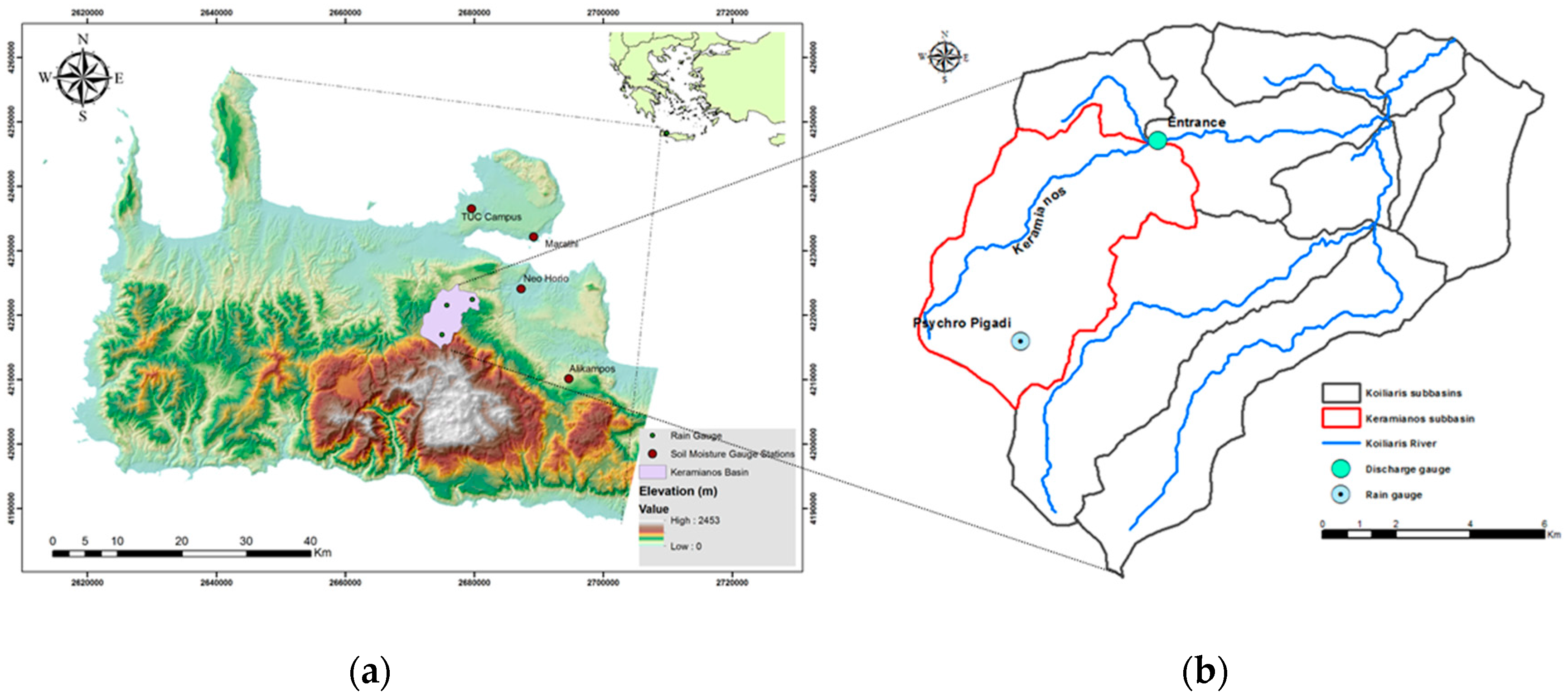
2. Case Study and Data
2.1. Earth Observation Data
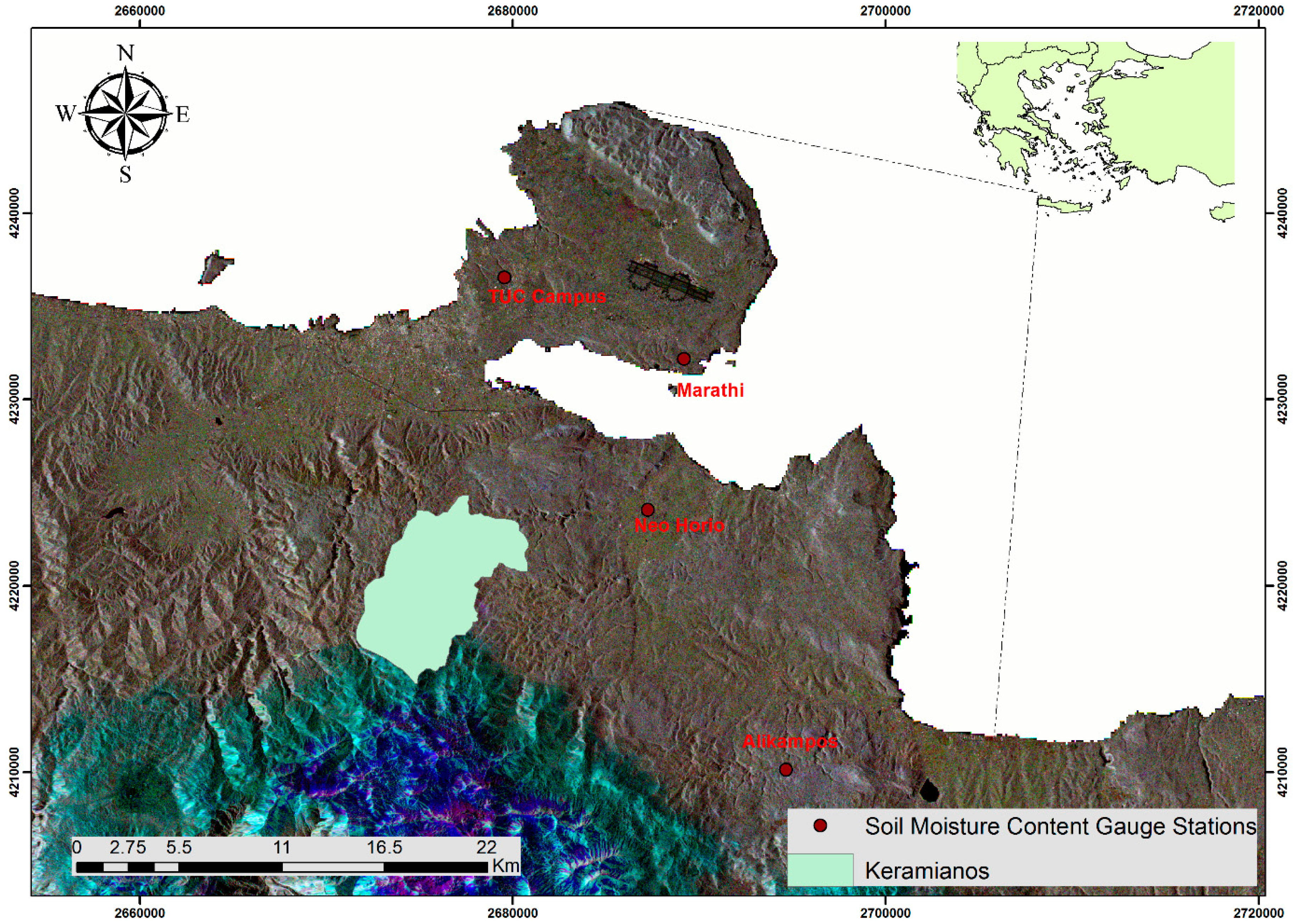
2.2. Ground Data
3. Methodology
3.1. ANN Approach
3.2. Hydrological Model
4. Results and Discussion
5. Conclusions
Acknowledgments
Author Contributions
Conflicts of Interest
References
- Baghdadi, N.; Aubert, M.; Cerdan, O.; Franchistéguy, L.; Viel, C.; Eric, M.; Zribi, M.; Desprats, J.F. Operational Mapping of Soil Moisture Using Synthetic Aperture Radar Data: Application to the Touch Basin (France). Sensors 2007, 7, 2458–2483. [Google Scholar] [CrossRef]
- Zhang, D.; Zhou, G. Estimation of Soil Moisture from Optical and Thermal Remote Sensing: A Review. Sensors 2016, 16, 1308. [Google Scholar] [CrossRef] [PubMed]
- Petropoulos, G.P.; Ireland, G.; Barrett, B. Surface soil moisture retrievals from remote sensing: Current status, products & future trends. Phys. Chem. Earth Parts A/B/C 2015, 83–84, 36–56. [Google Scholar]
- Ulaby, F.T.; Moore, R.K.; Fung, A.K. Microwave Remote Sensing: Active and Passive Volume II: Radar Remote Sensing and Surface Scattering and Emission Theory; Artech House Publishers: London, UK, 1982; Volume 2. [Google Scholar]
- Macelloni, G.; Paloscia, S.; Pampaloni, P.; Sigismondi, S.; De Matthaeis, P.; Ferrazzoli, P.; Schiavon, G.; Solimini, D. The SIR-C/X-SAR experiment on Montespertoli: Sensitivity to hydrological parameters. Int. J. Remote Sens. 1999, 20, 2597–2612. [Google Scholar] [CrossRef]
- Paloscia, S.; Pampaloni, P.; Pettinato, S.; Santi, E. A Comparison of Algorithms for Retrieving Soil Moisture from ENVISAT/ASAR Images. IEEE Trans. Geosci. Remote Sens. 2008, 46, 3274–3284. [Google Scholar] [CrossRef]
- Shi, J.; Chen, K.S.; Li, Q.; Jackson, T.J.; O’Neill, P.E.; Tsang, L. A parameterized surface reflectivity model and estimation of bare-surface soil moisture with L-band radiometer. IEEE Trans. Geosci. Remote Sens. 2002, 40, 2674–2686. [Google Scholar]
- Fernández-Prieto, D.; Kesselmeier, J.; Ellis, M.; Marconcini, M.; Reissell, A.; Suni, T. Preface “earth observation for land-Atmosphere interaction science”. Biogeosciences 2013, 10, 261–266. [Google Scholar] [CrossRef]
- Grillakis, M.G.; Koutroulis, A.G.; Komma, J.; Tsanis, I.K.; Wagner, W.; Blöschl, G. Initial soil moisture effects on flash flood generation—A comparison between basins of contrasting hydro-climatic conditions. J. Hydrol. 2016, 541, 206–217. [Google Scholar] [CrossRef]
- Gorrab, A.; Zribi, M.; Baghdadi, N.; Mougenot, B.; Fanise, P.; Chabaane, Z. Retrieval of Both Soil Moisture and Texture Using TerraSAR-X Images. Remote Sens. 2015, 7, 10098–10116. [Google Scholar] [CrossRef]
- Mattia, F. Using a priori information to improve soil moisture retrieval from ENVISAT ASAR AP in semi-arid regions. Sist. Intell. 2005, 44, 1–42. [Google Scholar]
- Mattia, F.; Le Toan, T.; Souyris, J.C.; De Carolis, C.; Floury, N.; Posa, F.; Pasquariello, N.G. The effect of surface roughness on multifrequency polarimetric SAR data. Geosci. Remote Sen. IEEE Trans. 1997, 35, 954–966. [Google Scholar] [CrossRef]
- Lievens, H.; Verhoest, N.E.C. Spatial and temporal soil moisture estimation from RADARSAT-2 imagery over Flevoland, The Netherlands. J. Hydrol. 2012, 456–457, 44–56. [Google Scholar] [CrossRef]
- Paloscia, S.; Pettinato, S.; Santi, E.; Notarnicola, C.; Pasolli, L.; Reppucci, A. Soil moisture mapping using Sentinel-1 images: Algorithm and preliminary validation. Remote Sens. Environ. 2013, 134, 234–248. [Google Scholar] [CrossRef]
- Doubková, M.; Van Dijk, A.I.J.M.; Sabel, D.; Wagner, W.; Blöschl, G. Evaluation of the predicted error of the soil moisture retrieval from C-band SAR by comparison against modelled soil moisture estimates over Australia. Remote Sens. Environ. 2012, 120, 188–196. [Google Scholar] [CrossRef] [PubMed]
- Gruber, A.; Wagner, W.; Hegyiova, A.; Greifeneder, F.; Schlaffer, S. Potential of Sentinel-1 for high-resolution soil moisture monitoring. In 2013 IEEE International Geoscience and Remote Sensing Symposium-IGARSS; IEEE: Melbourne, Australia, 2013; pp. 4030–4033. [Google Scholar]
- Wagner, W.; Lemoine, G.; Borgeaud, M.; Rott, H. A study of vegetation cover effects on ers scatterometer data. IEEE Transactions on Geoscience and Remote Sensing 1999, 37, 938–948. [Google Scholar] [CrossRef]
- Zribi, M.; Chahbi, A.; Shabou, M.; Lili-Chabaane, Z.; Duchemin, B.; Baghdadi, N.; Amri, R.; Chehbouni, A. Soil surface moisture estimation over a semi-arid region using ENVISAT ASAR radar data for soil evaporation evaluation. Hydrol. Earth Syst. Sci. 2011, 15, 345–358. [Google Scholar] [CrossRef]
- Mattia, F.; Satalino, G.; Balenzano, A.; Rinaldi, M.; Steduto, P.; Moreno, J. Sentinel-1 for wheat mapping and soil moisture retrieval. In Proceedings of the 2015 IEEE International Geoscience and Remote Sensing Symposium (IGARSS), Milan, Italy, 26–31 July 2015; pp. 2832–2835. [Google Scholar]
- Santi, E.; Pettinato, S.; Paloscia, S.; Pampaloni, P.; Macelloni, G.; Brogioni, M. An algorithm for generating soil moisture and snow depth maps from microwave spaceborne radiometers: HydroAlgo. Hydrol. Earth Syst. Sci. 2012, 16, 3659–3676. [Google Scholar] [CrossRef]
- Balenzano, A.; Mattia, F.; Satalino, G.; Pauwels, V.; Snoeij, P. SMOSAR algorithm for soil moisture retrieval using Sentinel-1 data. In Proceedings of the 2012 IEEE International Geoscience and Remote Sensing Symposium (IGARSS), Munich, Germany, 22–27 July 2012; pp. 1200–1203. [Google Scholar]
- Ahmad, S.; Kalra, A.; Stephen, H. Estimating soil moisture using remote sensing data: A machine learning approach. Adv. Water Res. 2010, 33, 69–80. [Google Scholar] [CrossRef]
- Choker, M.; Baghdadi, N.; Zribi, M.; El Hajj, M.; Paloscia, S.; Verhoest, N.; Lievens, H.; Mattia, F. Evaluation of the Oh, Dubois and IEM Backscatter Models Using a Large Dataset of SAR Data and Experimental Soil Measurements. Water 2017, 9, 38. [Google Scholar] [CrossRef]
- Fung, A.K.; Chen, K.S. An update on the IEM surface backscattering model. IEEE Geosci. Remote Sens. Lett. 2004, 1, 75–77. [Google Scholar] [CrossRef]
- He, B.; Xing, M.; Bai, X. A Synergistic Methodology for Soil Moisture Estimation in an Alpine Prairie Using Radar and Optical Satellite Data. Remote Sens. 2014, 6, 10966–10985. [Google Scholar] [CrossRef]
- Wu, T.D.; Chen, K.S. A reappraisal of the validity of the IEM model for backscattering from rough surfaces. IEEE Trans. Geosci. Remote Sens. 2004, 42, 743–753. [Google Scholar]
- Pierdicca, N.; Pulvirenti, L.; Bignami, C. Soil moisture estimation over vegetated terrains using multitemporal remote sensing data. Remote Sens. Environ. 2010, 114, 440–448. [Google Scholar] [CrossRef]
- Oh, Y.; Sarabandi, K.; Ulaby, F.T. An empirical model and an inversion technique for radar scattering from bare soil surfaces. IEEE Trans. Geosci. Remote Sens. 1992, 30, 370–381. [Google Scholar] [CrossRef]
- Dubois, P.C.; van Zyl, J.; Engman, T. Measuring soil moisture with imaging radars. IEEE Trans. Geosci. Remote Sens. 1995, 33, 915–926. [Google Scholar] [CrossRef]
- Filion, R.; Bernier, M.; Paniconi, C.; Chokmani, K.; Melis, M.; Soddu, A.; Talazac, M.; Lafortune, F.-X. Remote sensing for mapping soil moisture and drainage potential in semi-arid regions: Applications to the Campidano plain of Sardinia, Italy. Sci. Total Environ. 2016, 543, 862–876. [Google Scholar] [CrossRef] [PubMed]
- Parajka, J.; Naeimi, V.; Blöschl, G.; Komma, J. Matching ERS scatterometer based soil moisture patterns with simulations of a conceptual dual layer hydrologic model over Austria. Hydrol. Earth Syst. Sci. Discuss. 2008, 5, 3313–3353. [Google Scholar] [CrossRef]
- Salvucci, G.D.; Entekhabi, D. An alternate and robust approach to calibration for the estimation of land surface model parameters based on remotely sensed observations. Geophys. Res. Lett. 2011, 38, 1–6. [Google Scholar] [CrossRef]
- Gorrab, A.; Simonneaux, V.; Zribi, M.; Saadi, S.; Baghdadi, N.; Lili Chabaane, Z.; Fanise, P. Bare soil hydrological balance model “MHYSAN”: Calibration and validation using SAR moisture products and continuous thetaprobe network measurements over bare agricultural soils (Tunisia). J. Arid Environ. 2017, 139, 11–25. [Google Scholar] [CrossRef]
- EL Hajj, M.; Baghdadi, N.; Cheviron, B.; Belaud, G.; Zribi, M. Integration of remote sensing derived parameters in crop models: Application to the PILOTE model for hay production. Agric. Water Manag. 2016, 176, 67–79. [Google Scholar] [CrossRef]
- Xu, X.; Li, J.; Tolson, B.A. Progress in integrating remote sensing data and hydrologic modeling. Prog. Phys. Geogr. 2014, 38, 464–498. [Google Scholar] [CrossRef]
- Scharffenberg, W. Hydrologic Modeling System HEC-HMS : User’s Manual; US Army Corps of Engineers Hydrologic Engineering Center: Davis, CA, USA, 2006. [Google Scholar]
- Alexakis, D.D.; Sarris, A. Integrated GIS and remote sensing analysis for landfill sitting in Western Crete, Greece. Environ. Earth Sci. 2014, 72, 467–482. [Google Scholar] [CrossRef]
- Moraetis, D.; Stamati, F.; Kotronakis, M.; Fragia, T.; Paranychnianakis, N.; Nikolaidis, N.P. Identification of hydrologic and geochemical pathways using high frequency sampling, REE aqueous sampling and soil characterization at Koiliaris Critical Zone Observatory, Crete. Appl. Geochem. 2011, 26, S101–S104. [Google Scholar] [CrossRef]
- Nikolaidis, N.P.; Bouraoui, F.; Bidoglio, G. Hydrologic and geochemical modeling of a karstic Mediterranean watershed. Hydrol. Earth Syst. Sci. Discuss. 2012, 9, 1–27. [Google Scholar] [CrossRef]
- Nerantzaki, S.D.; Giannakis, G.V.; Efstathiou, D.; Nikolaidis, N.P.; Sibetheros, I.A.; Karatzas, G.P.; Zacharias, I. Modeling suspended sediment transport and assessing the impacts of climate change in a karstic Mediterranean watershed. Sci. Total Environ. 2015, 538, 288–297. [Google Scholar] [CrossRef] [PubMed]
- Vozinaki, A.-E.K.; Karatzas, G.P.; Sibetheros, I.A.; Varouchakis, E.A. An agricultural flash flood loss estimation methodology: The case study of the Koiliaris basin (Greece), February 2003 flood. Nat. Hazard. 2015, 79, 899–920. [Google Scholar] [CrossRef]
- Torres, R.; Snoeij, P.; Geudtner, D.; Bibby, D.; Davidson, M.; Attema, E.; Potin, P.; Rommen, B.; Floury, N.; Brown, M.; et al. GMES Sentinel-1 mission. Remote Sens. Environ. 2012, 120, 9–24. [Google Scholar] [CrossRef]
- Baghdadi, N.; King, C.; Bonnifait, A. An empirical calibration of the integral equation model based on SAR data and soil parameters measurements. IEEE Int. Geosci. Remote Sens. Symp. 2002, 5, 2646–2650. [Google Scholar]
- Panciera, R.; Walker, J.P.; Jackson, T.J.; Gray, D.A.; Tanase, M.A.; Ryu, D.; Monerris, A.; Yardley, H.; Rudiger, C.; Wu, X.; et al. The Soil Moisture Active Passive Experiments (SMAPEx): Toward Soil Moisture Retrieval From the SMAP Mission. IEEE Trans. Geosci. Remote Sens. 2014, 52, 490–507. [Google Scholar] [CrossRef]
- Leconte, R.; Brissette, F.; Galarneau, M.; Rousselle, J. Mapping near-surface soil moisture with RADARSAT-1 synthetic aperture radar data. Water Res. Res. 2004, 40. [Google Scholar] [CrossRef]
- Topp, G.C.; Davis, J.L.; Annan, A.P. Electromagnetic determination of soil water content: Measurements in coaxial transmission lines. Water Res. Res. 1980, 16, 574–582. [Google Scholar] [CrossRef]
- Agapiou, A.; Hadjimitsis, D.G.; Papoutsa, C.; Alexakis, D.D.; Papadavid, G. The Importance of accounting for atmospheric effects in the application of NDVI and interpretation of satellite imagery supporting archaeological research: The case studies of Palaepaphos and Nea Paphos sites in Cyprus. Remote Sens. 2011, 3, 2605–2629. [Google Scholar] [CrossRef]
- Zhang, T.; Wen, J.; Su, Z.; Velde, R.V.D.; Timmermans, J.; Liu, R.; Liu, Y.; Li, Z. Soil moisture mapping over the Chinese Loess Plateau using ENVISAT/ASAR data. Adv. Space Res. 2009, 43, 1111–1117. [Google Scholar] [CrossRef]
- Sun, C.; Liu, Y.; Zhao, S.; Zhou, M.; Yang, Y.; Li, F. Classification mapping and species identification of salt marshes based on a short-time interval NDVI time-series from HJ-1 optical imagery. Int. J. Appl. Earth Obs. Geoinf. 2016, 45, 27–41. [Google Scholar] [CrossRef]
- Wang, H.; Li, X.; Long, H.; Xu, X.; Bao, Y. Monitoring the effects of land use and cover type changes on soil moisture using remote-sensing data: A case study in China’s Yongding River basin. CATENA 2010, 82, 135–145. [Google Scholar] [CrossRef]
- Shafian, S.; Maas, S. Index of Soil Moisture Using Raw Landsat Image Digital Count Data in Texas High Plains. Remote Sens. 2015, 7, 2352–2372. [Google Scholar] [CrossRef]
- Czarnomski, N.M.; Moore, G.W.; Pypker, T.G.; Licata, J.; Bond, B.J. Precision and accuracy of three alternative instruments for measuring soil water content in two forest soils of the Pacific Northwest. Can. J. For. Res. 2005, 35, 1867–1876. [Google Scholar] [CrossRef]
- Wang, J.; Ling, Z.; Wang, Y.; Zeng, H. Improving spatial representation of soil moisture by integration of microwave observations and the temperature–vegetation–drought index derived from MODIS products. ISPRS J. Photogr. Remote Sens. 2016, 113, 144–154. [Google Scholar] [CrossRef]
- Zribi, M.; Dechambre, M. A new empirical model to retrieve soil moisture and roughness from C-band radar data. Remote Sens. Environ. 2003, 84, 42–52. [Google Scholar] [CrossRef]
- Hornik, K.; Stinchcombe, M.; White, H. Multilayer feedforward networks are universal approximators. Neural Netw. 1989, 2, 359–366. [Google Scholar] [CrossRef]
- Linden, A.; Kindermann, J. Inversion of multilayer nets. Int. Jt. Conference Neural Netw. 1989, 2, 425–430. [Google Scholar]
- Tapoglou, E.; Karatzas, G.P.; Trichakis, I.C.; Varouchakis, E.A. A spatio-temporal hybrid neural network-Kriging model for groundwater level simulation. J. Hydrol. 2014, 519, 3193–3203. [Google Scholar] [CrossRef]
- Santi, E.; Paloscia, S.; Pettinato, S.; Fontanelli, G. Application of artificial neural networks for the soil moisture retrieval from active and passive microwave spaceborne sensors. Int. J. Appl. Earth Obs. Geoinf. 2016, 48, 61–73. [Google Scholar] [CrossRef]
- Kia, M.B.; Pirasteh, S.; Pradhan, B.; Mahmud, A.R.; Sulaiman, W.N.A.; Moradi, A. An artificial neural network model for flood simulation using GIS: Johor River Basin, Malaysia. Environ. Earth Sci. 2012, 67, 251–264. [Google Scholar] [CrossRef]
- Daliakopoulos, I.N.; Tsanis, I.K. Comparison of an artificial neural network and a conceptual rainfall–runoff model in the simulation of ephemeral streamflow. Hydrol. Sci. J. 2016. [Google Scholar] [CrossRef]
- Tsiknia, M.; Paranychianakis, N.V.; Varouchakis, E.A.; Moraetis, D.; Nikolaidis, N.P. Environmental drivers of soil microbial community distribution at the Koiliaris Critical Zone Observatory. FEMS Microbiol. Ecol. 2014, 90, 139–152. [Google Scholar] [CrossRef] [PubMed]
- Tramblay, Y.; Bouvier, C.; Martin, C.; Didon-Lescot, J.F.; Todorovik, D.; Domergue, J.M. Assessment of initial soil moisture conditions for event-based rainfall-runoff modelling. J. Hydrol. 2010, 387, 176–187. [Google Scholar] [CrossRef]
- Nash, J.E.; Sutcliffe, J.V. River flow forecasting through conceptual models part I—Discussion of principles. J. Hydrol. 1970, 10, 282–290. [Google Scholar] [CrossRef]


| # | Sensor | Date of Acquisition | # | Sensor | Date of Acquisition |
|---|---|---|---|---|---|
| 1 | Landsat 8 | 9 February 2015 | 20 | Sentinel-1 | 23 April 2015 |
| 2 | Landsat 8 | 13 April 2015 | 21 | Sentinel-1 | 4 March 2015 |
| 3 | Landsat 8 | 29 April 2015 | 22 | Sentinel-1 | 5 March 2015 |
| 4 | Landsat 8 | 15 March 2015 | 23 | Sentinel-1 | 16 March 2015 |
| 5 | Landsat 8 | 31 March 2015 | 24 | Sentinel-1 | 17 March 2015 |
| 6 | Landsat 8 | 16 June 2015 | 25 | Sentinel-1 | 28 March 2015 |
| 7 | Landsat 8 | 18 July 2015 | 26 | Sentinel-1 | 29 March 2015 |
| 8 | Landsat 8 | 19 August 2015 | 27 | Sentinel-1 | 9 June 2015 |
| 9 | Landsat 8 | 20 September 2015 | 28 | Sentinel-1 | 21 June 2015 |
| 10 | Landsat 8 | 23 November 2015 | 29 | Sentinel-1 | 22 June 2015 |
| 11 | Landsat 8 | 25 December 2015 | 30 | Sentinel-1 | 3 July 2015 |
| 12 | Sentinel-1 | 16 January 2015 | 31 | Sentinel-1 | 4 July 2015 |
| 13 | Sentinel-1 | 17 January 2015 | 32 | Sentinel-1 | 27 July 2015 |
| 14 | Sentinel-1 | 9 February 2015 | 33 | Sentinel-1 | 28 July 2015 |
| 15 | Sentinel-1 | 29 March 2015 | 34 | Sentinel-1 | 8 August 2015 |
| 16 | Sentinel-1 | 30 March 2015 | 35 | Sentinel-1 | 25 September 2015 |
| 17 | Sentinel-1 | 10 April 2015 | 36 | Sentinel-1 | 7 October 2015 |
| 18 | Sentinel-1 | 11 April 2015 | 37 | Sentinel-1 | 24 November 2015 |
| 19 | Sentinel-1 | 22 April 2015 | 38 | Sentinel-1 | 18 December 2015 |
| Experimental Field | Distance from Sea (m) | Elevation (m) |
|---|---|---|
| Marathi | 450 | 52 |
| Neo Horio | 3000 | 36 |
| Alikampos | 6000 | 398 |
| TUC Campus | 1500 | 120 |
| # | Study Area | R2 | RMSE |
|---|---|---|---|
| 1 | Marathi | 0.867 | 0.022 |
| 2 | Neo Horio | 0.842 | 0.041 |
| 3 | Alikampos | 0.914 | 0.031 |
| 4 | TUC | 0.810 | 0.047 |
| 5 | Overall (All the study sites) | 0.500 | 0.042 |
| 6 | Study Areas: Neo Horio, Marathi, Alikampos | 0.829 | 0.040 |
| 7 | Study Areas: Neo Horio, TUC, Alikampos | 0.819 | 0.048 |
| 8 | Study Areas: Alikampos, Marathi, TUC | 0.657 | 0.033 |
| 9 | Study Areas: TUC, Marathi, Alikampos | 0.400 | 0.058 |
| Subtracted Parameter | Marathi | Neo Horio | Alikampos | TUC | All Fields | |||||
|---|---|---|---|---|---|---|---|---|---|---|
| R2 | RMSE | R2 | RMSE | R2 | RMSE | R2 | RMSE | R2 | RMSE | |
| 0.724 | 0.057 | 0.846 | 0.055 | 0.867 | 0.036 | 0.811 | 0.044 | 0.745 | 0.044 | |
| (−17%) | (+0.4) | (−6%) | (+50%) | |||||||
| NDVI | 0.338 | 0.052 | 0.569 | 0.059 | 0.506 | 0.072 | 0.552 | 0.082 | 0.349 | 0.069 |
| (−62%) | (−35%) | (−35%) | (−32%) | (31%) | ||||||
| TIRn | 0.774 | 0.039 | 0.895 | 0.028 | 0.664 | 0.066 | 0.781 | 0.053 | 0.509 | 0.062 |
| (−10%) | (+6%) | (−28%) | (−4%) | (+1.8%) | ||||||
| 0.788 | 0.034 | 0.87 | 0.032 | 0.857 | 0.035 | 0.843 | 0.041 | 0.746 | 0.051 | |
| (−9%) | (+3%) | (−7%) | (+4%) | (+50%) | ||||||
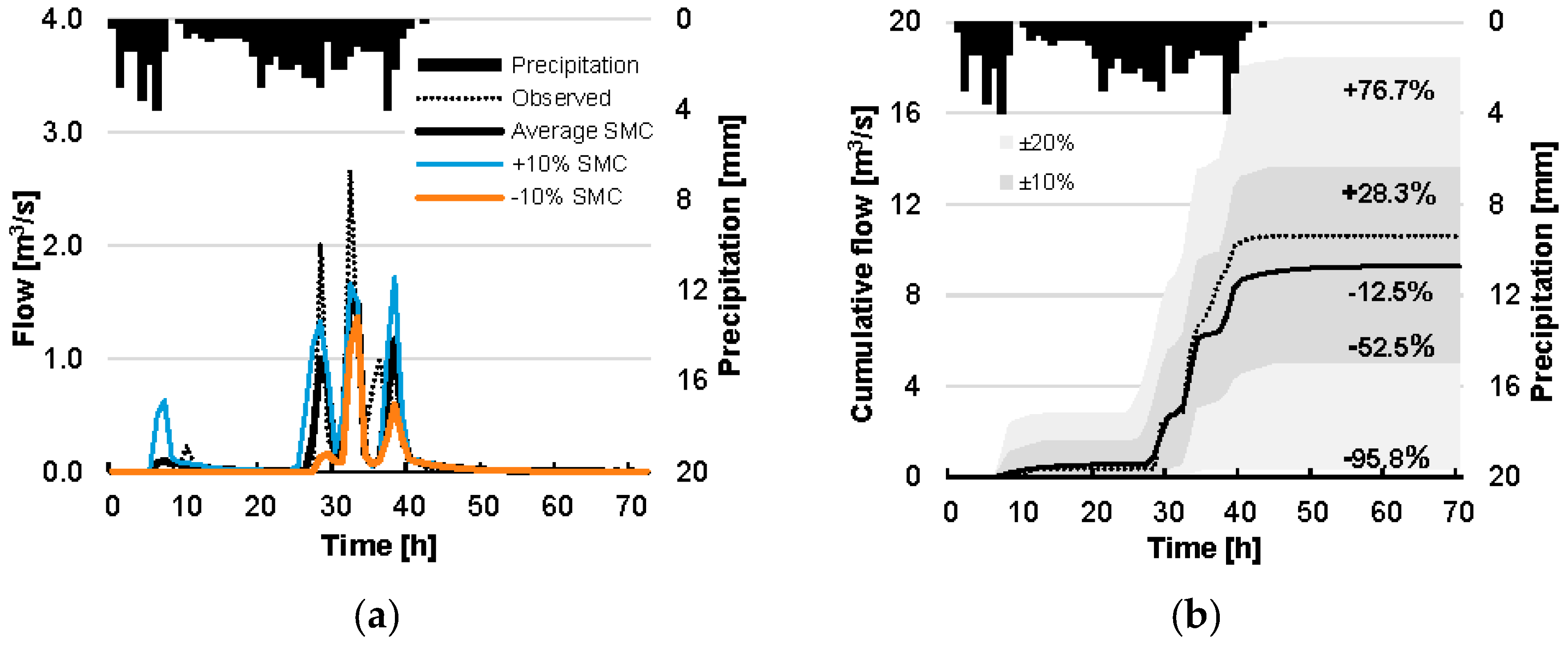
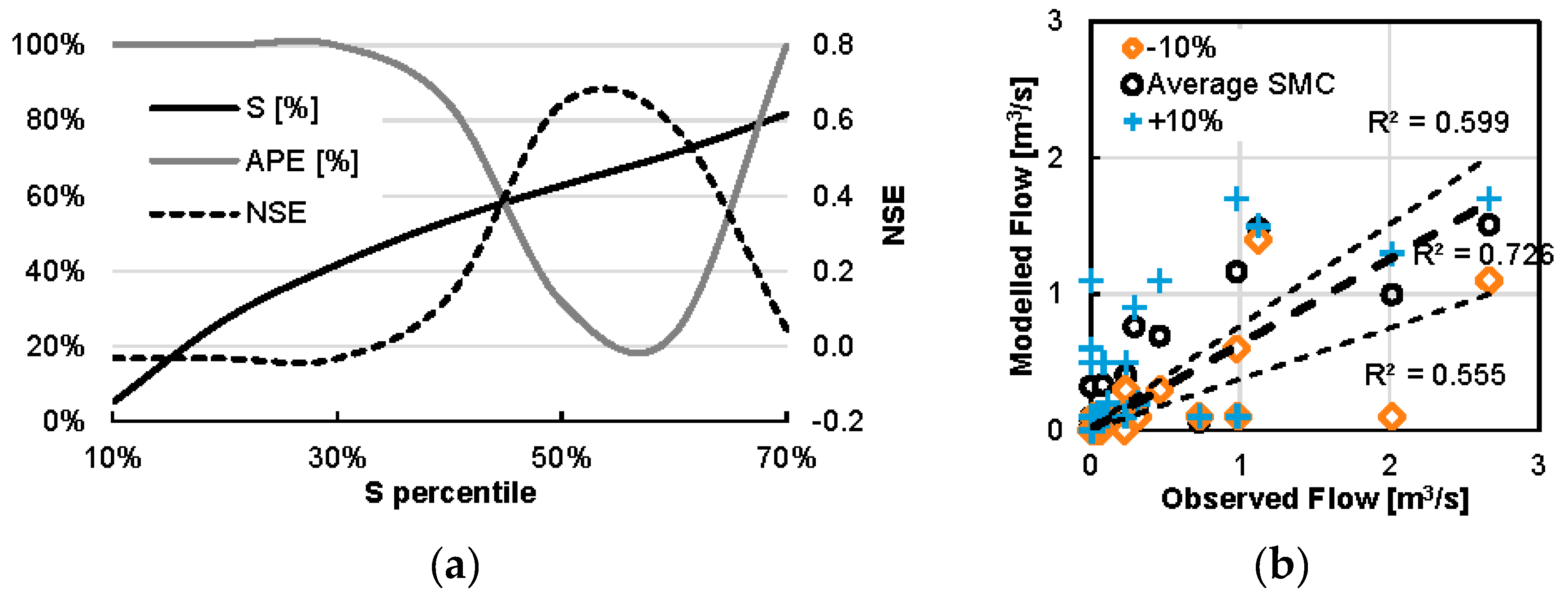
| SMC Scenario | Satellite SMC (m3 m−3) | Degree of Saturation, (%) | NSE | R2 | Simulated Equivalent Volume, Q (mm) | APE (%) |
|---|---|---|---|---|---|---|
| −20% | 0.2667 | 52.4 | 0.016 | 0.356 | 0.05 | 95.8 |
| −10% | 0.3001 | 58.9 | 0.494 | 0.555 | 0.57 | 52.5 |
| Average SMC | 0.3334 | 65.5 | 0.712 | 0.726 | 1.05 | 12.5 |
| +10% | 0.3667 | 72.0 | 0.556 | 0.599 | 1.54 | 28.3 |
| +20% | 0.4001 | 78.5 | 0.253 | 0.525 | 2.12 | 76.7 |
© 2017 by the authors. Licensee MDPI, Basel, Switzerland. This article is an open access article distributed under the terms and conditions of the Creative Commons Attribution (CC BY) license (http://creativecommons.org/licenses/by/4.0/).
Share and Cite
Alexakis, D.D.; Mexis, F.-D.K.; Vozinaki, A.-E.K.; Daliakopoulos, I.N.; Tsanis, I.K. Soil Moisture Content Estimation Based on Sentinel-1 and Auxiliary Earth Observation Products. A Hydrological Approach. Sensors 2017, 17, 1455. https://doi.org/10.3390/s17061455
Alexakis DD, Mexis F-DK, Vozinaki A-EK, Daliakopoulos IN, Tsanis IK. Soil Moisture Content Estimation Based on Sentinel-1 and Auxiliary Earth Observation Products. A Hydrological Approach. Sensors. 2017; 17(6):1455. https://doi.org/10.3390/s17061455
Chicago/Turabian StyleAlexakis, Dimitrios D., Filippos-Dimitrios K. Mexis, Anthi-Eirini K. Vozinaki, Ioannis N. Daliakopoulos, and Ioannis K. Tsanis. 2017. "Soil Moisture Content Estimation Based on Sentinel-1 and Auxiliary Earth Observation Products. A Hydrological Approach" Sensors 17, no. 6: 1455. https://doi.org/10.3390/s17061455