
3D Imaging of Rapidly Spinning Space Targets Based on a Factorization Method


Abstract
:1. Introduction
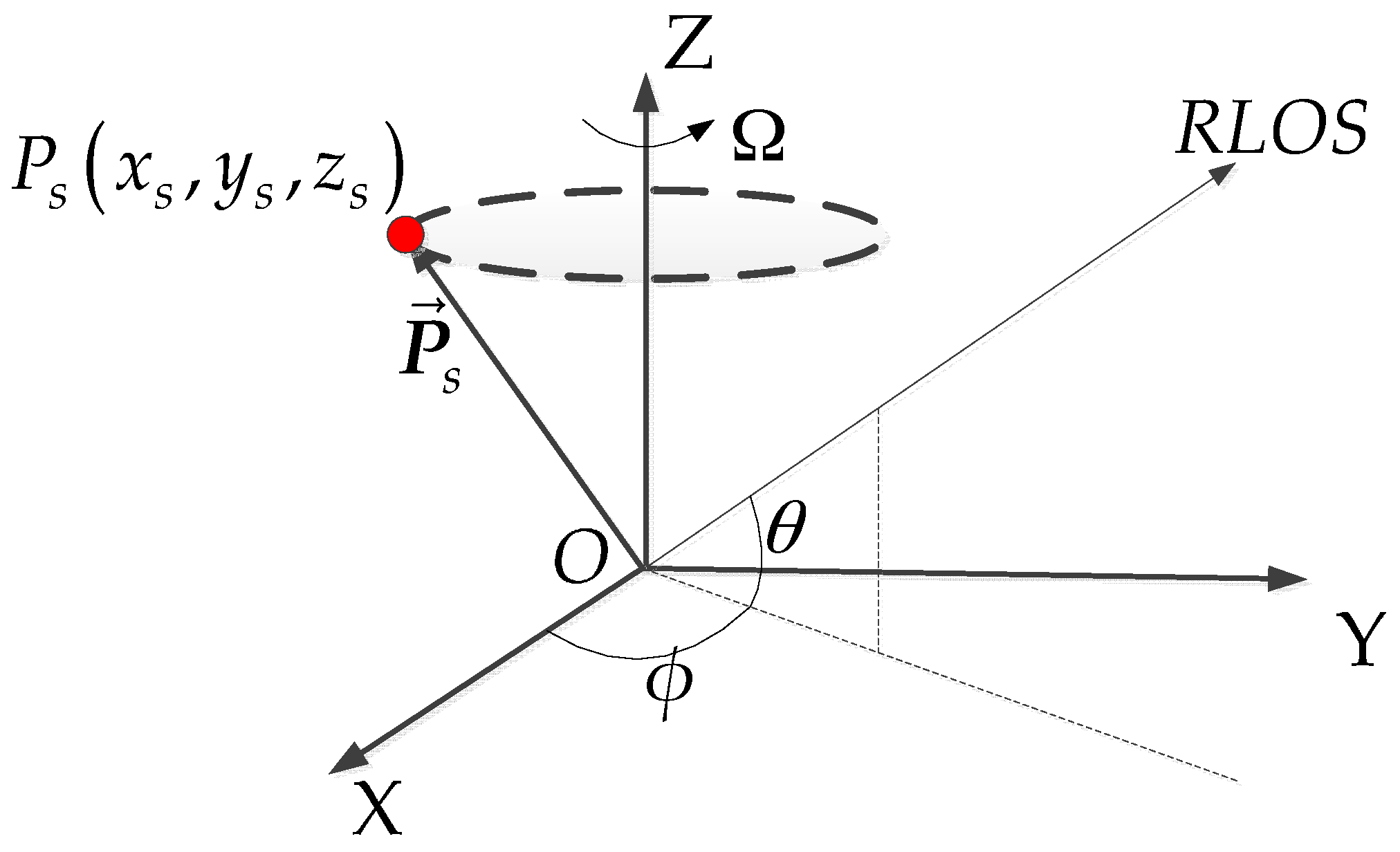
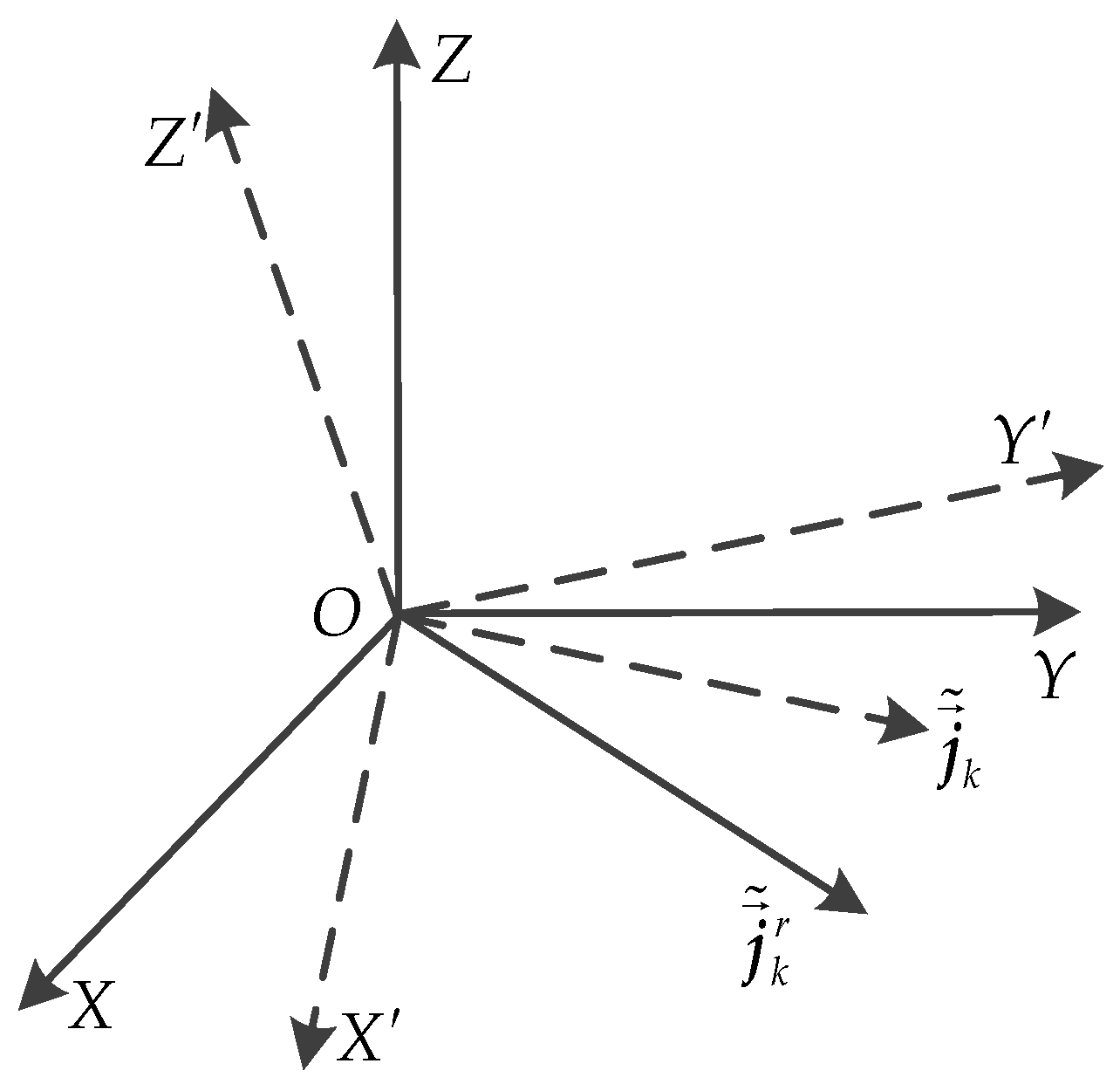
2. Imaging Geometry
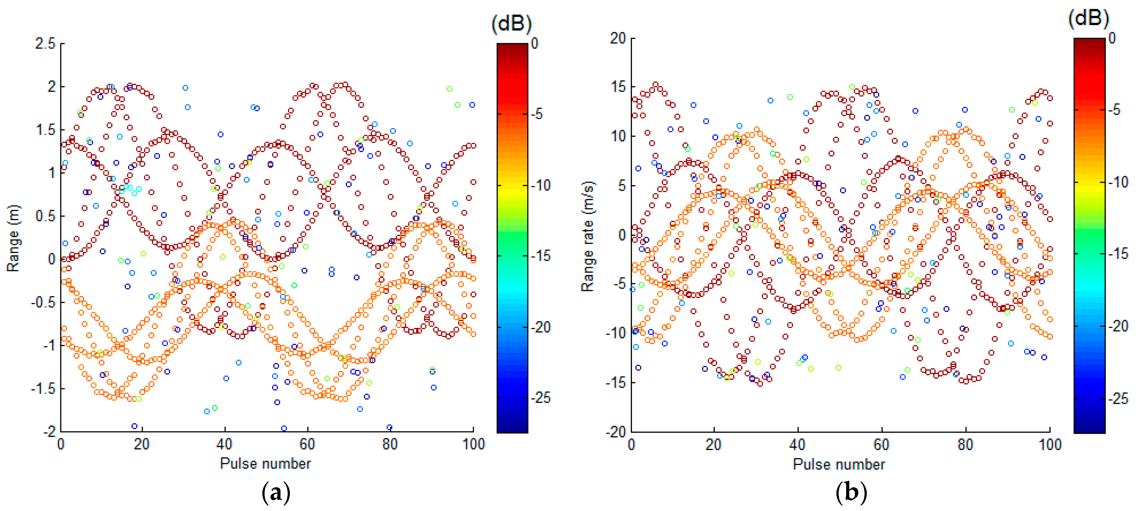
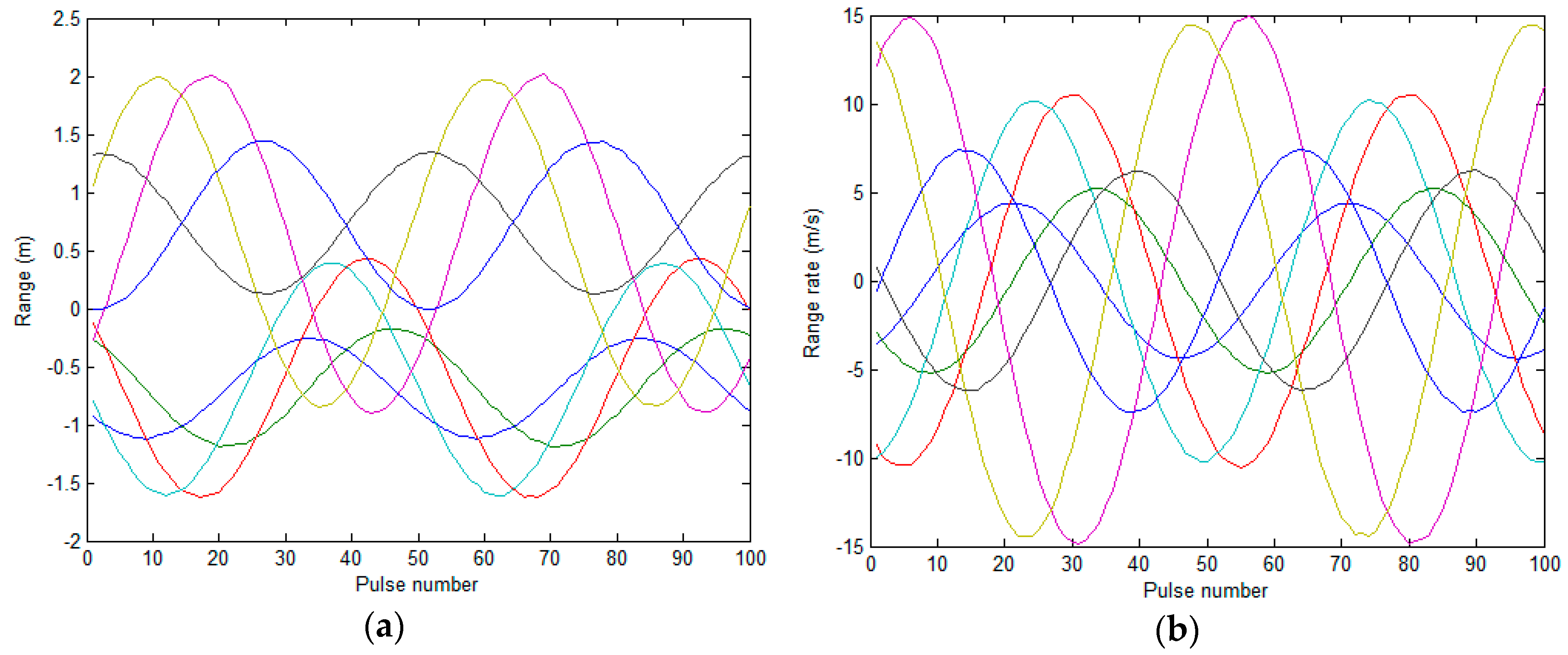
3. Feature Extraction
4. Scattering Center Association
- Step 1:
- Initialization. Let m = 1.
- Step 2:
- For the m-th range and range-rate, we have the measurements , where is the scattering center track index, is the amplitude estimate. Define the initial measurements as .
- Step 1:
- Initialization. Let m = 1.
- Step 2:
- For the m-th range and range-rate, we have the measurements , where i is the scattering center track index, Ai,m is the amplitude estimate. We define the initial measurements as .
- Step 3:
- Let m = m + 1. For the i-th scattering center track, search for the candidate scattering centers within the search window centered at ri,m−1, then record the candidate set . Here, for a small observation interval, we assume the amplitude difference between the adjacent observation times is very small, so the optimal candidate for the i-th track can be determined by:The other tracks are similarly associated with the scattering centers according to Equation (23). The acceleration of the scattering centers can be calculated as follows:Now, the initial state vector can be denoted as . Then, the next state can be obtained according to Equations (19) to (21).
- Step 4:
- Move to the next time index and let . According to the minimum Euclidean distance criterion [23], the optimal candidate of the scattering center track for the m-th range can be obtained by:where is the feature set of the candidate scattering centers within the gating area and are the features of the predictions from the previous observables. can be expressed as:where , and are weight factors and . According to Equations (23) and (26), Equation (25) can be rewritten as:Finally, by using Equation (30), the scattering centres association is accomplished.
- Step 5:
- Repeat Step 4 to finish the whole measurements association.
5. Factorization-Based 3D Imaging and Scaling
5.1. 3D Imaging Based on Factorization Method
5.2. 3D Image Scaling
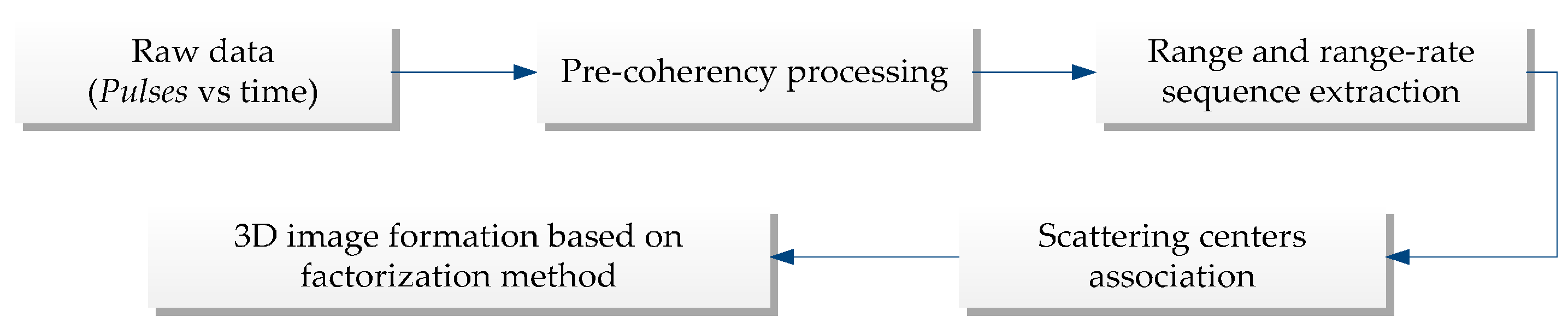
| Algorithm 1: Processing steps of the proposed method |
| Input: Raw data |
| Pre-processing: -Apply the pre-coherency processing [25] to the data -Extract the range and range-rate using the spectral estimate method [22] -Correlate the range and range-rate sequenceusing method developed in Section 4 |
| Initialization: initialize k = 0, and choose an initial coarse angluar velocity and the error threshold . Perform scaling to the sequential range-rate to form the projection matrix W0 according to Equations (3), (4) and (8) |
| Main iteration: increase k by 1 and perform the following procedure: |
| Step 1: Submit to Equation (4) to rescale the cross-range and obtain the scaled matrix Wk |
| Step 2: Calculate the motion matrix and shape matrix by substituting Wk into Equations (32) and (33) |
| Step 3: According to Equations (42)−(45) and the result in Step 2, calculate the rotational transform matrix Qk |
| Step 4: Estimate the angular velocity by substituting Qk into Equations (46)−(48) |
| Step 5: If , then , and stop the iteration. Otherwise, repeat the main iteration. |
| Output: Estimate . Consequently, the well-scaled shape matrix can be generated using the optimal . |
6. Simulation Results
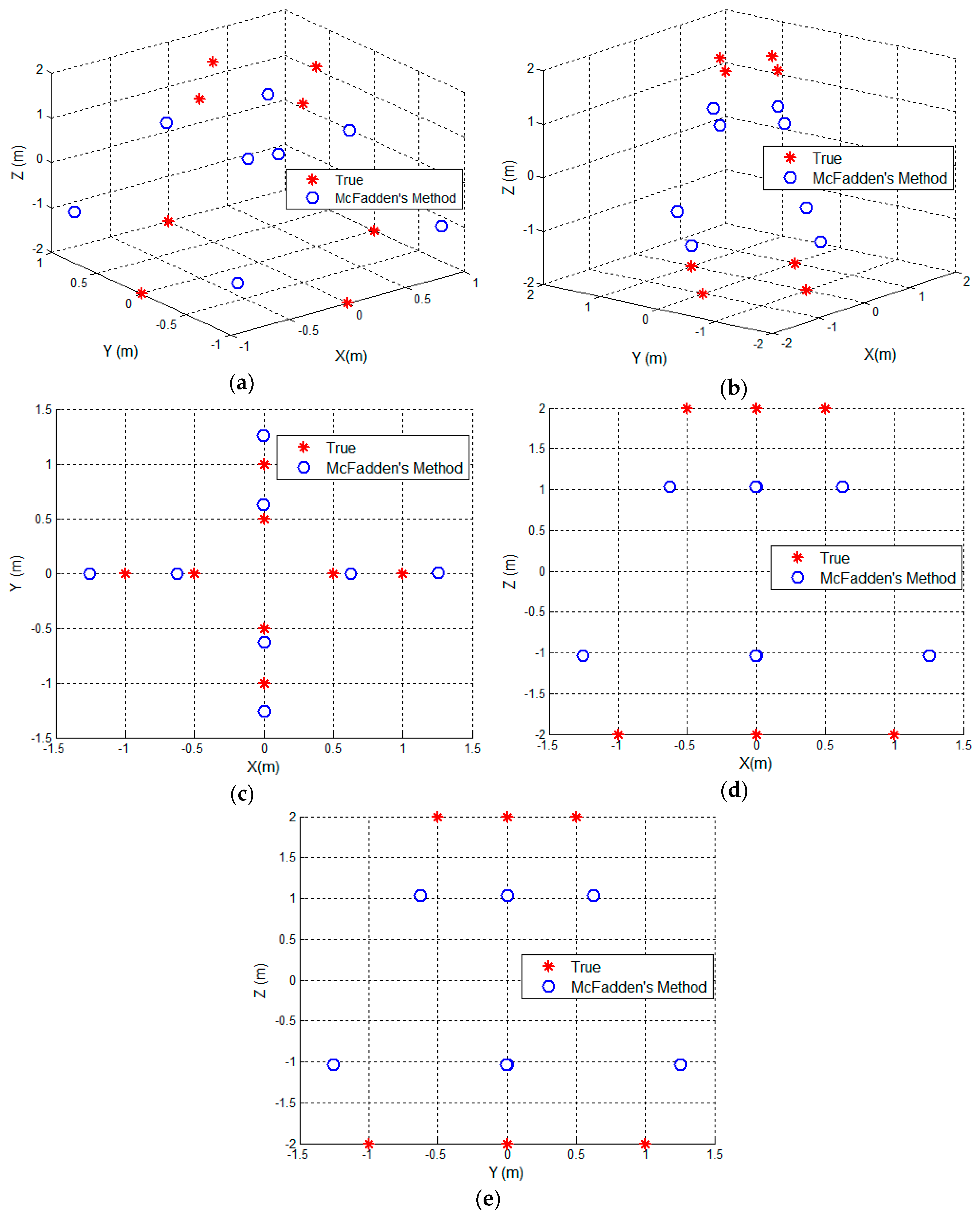
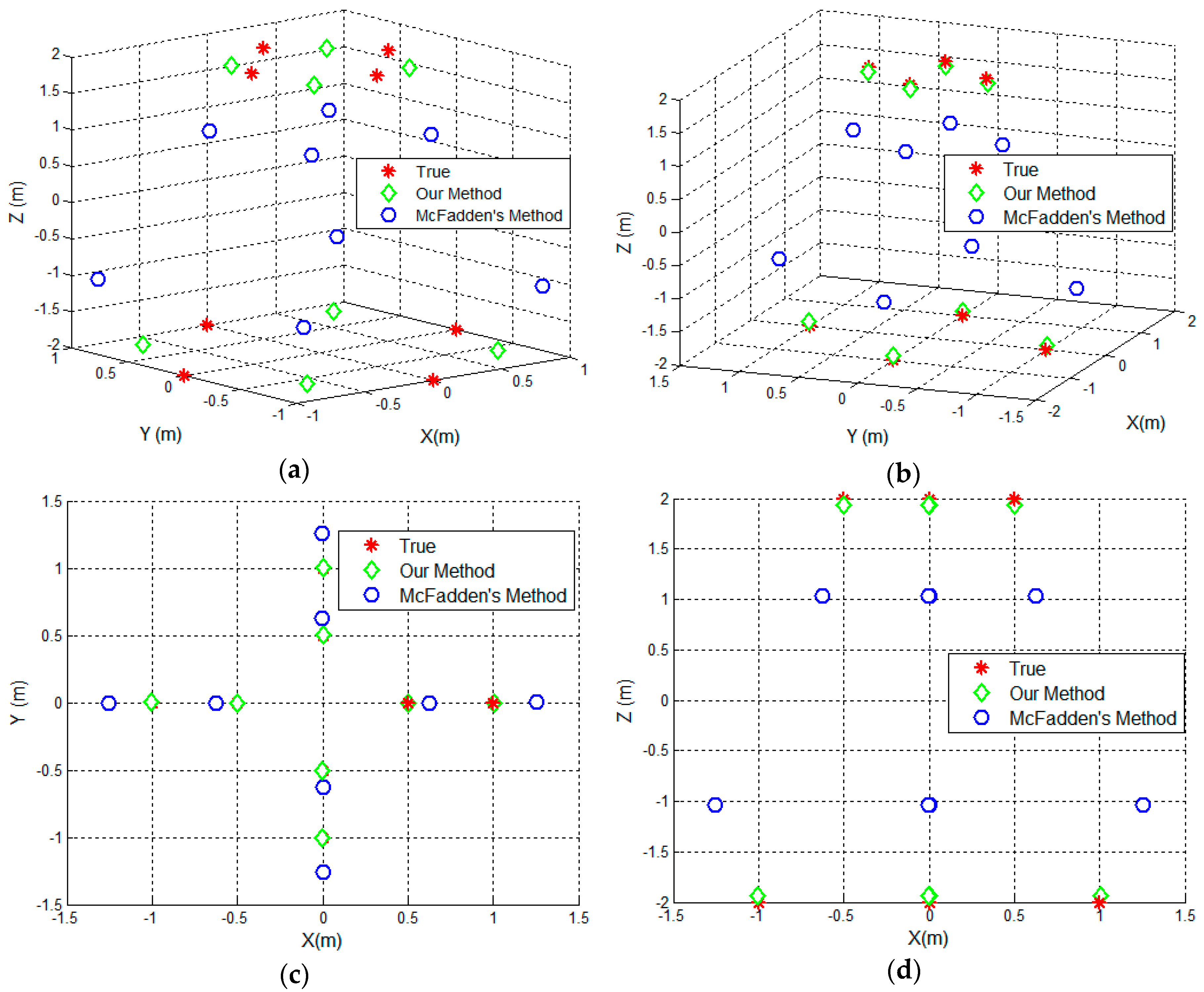
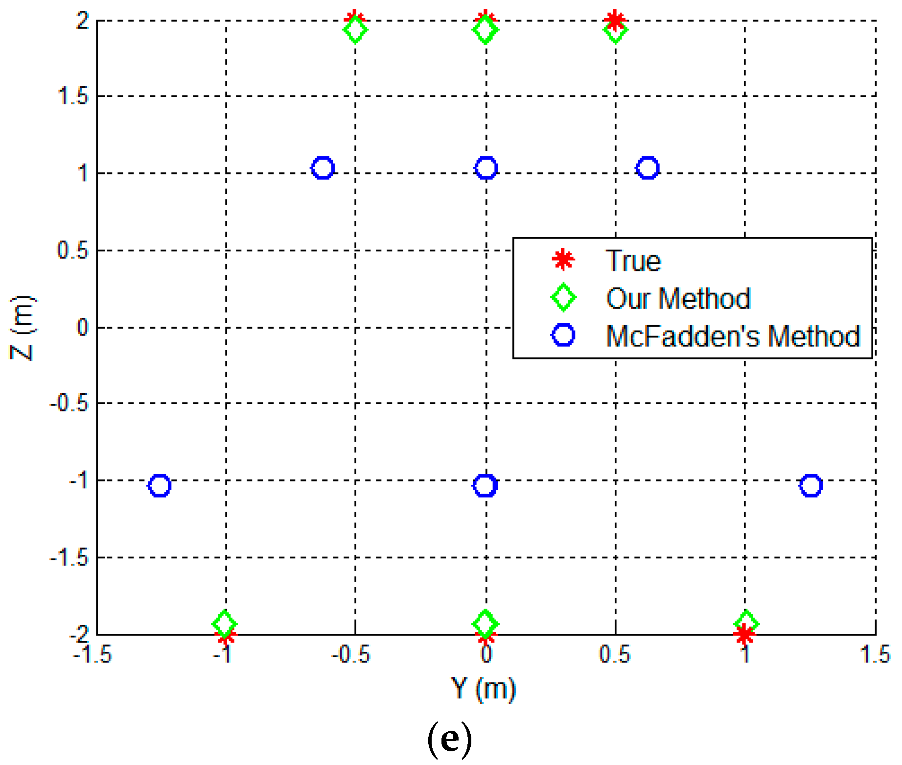
6.1. Simulation Results
6.2. Performance Analysis
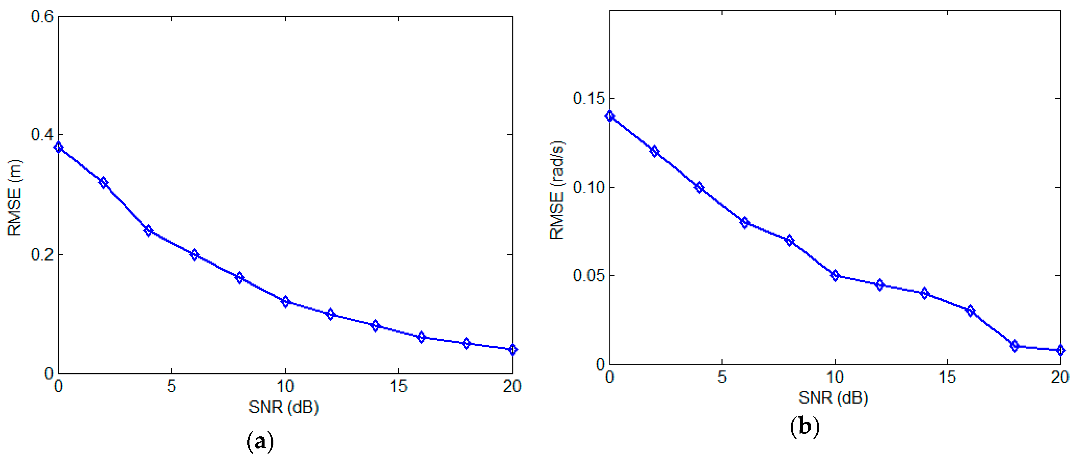
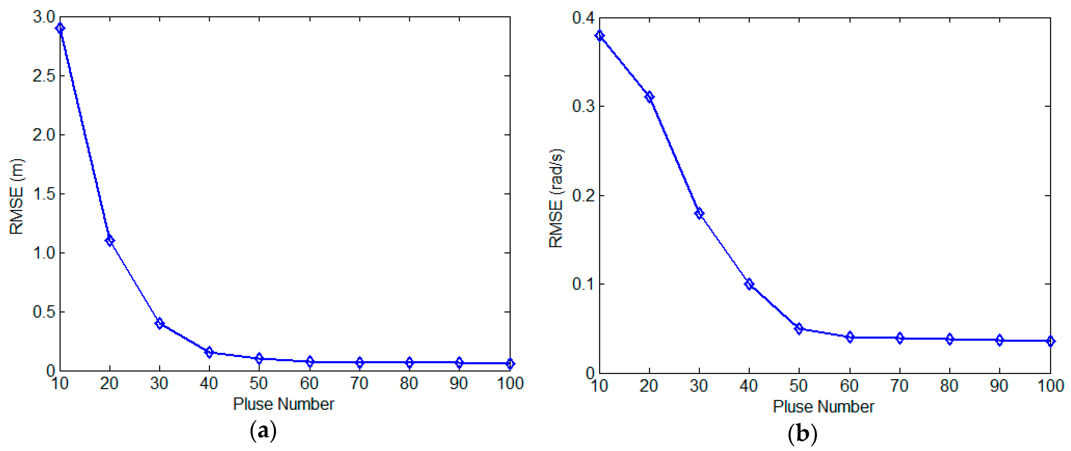
6.2.1. Effect of the SNR Level and Pulse Quantity
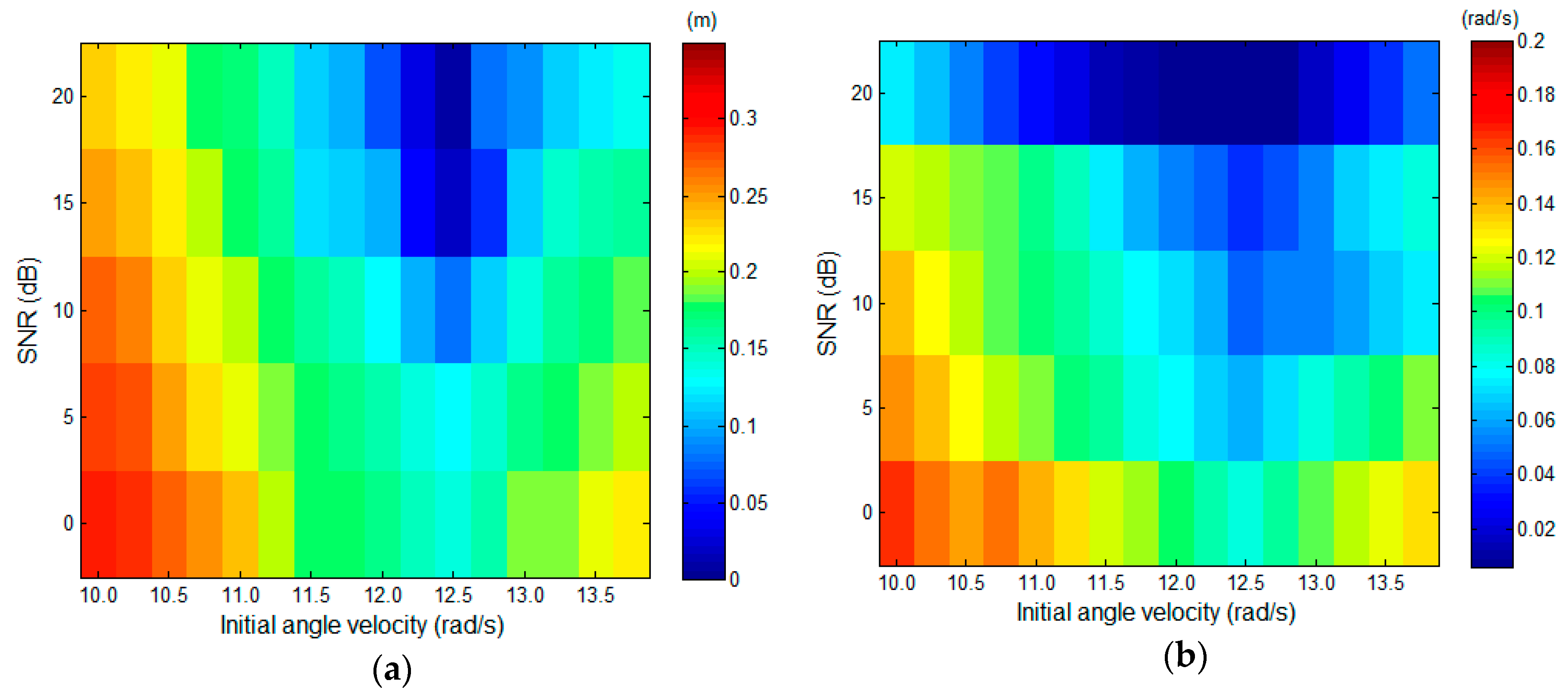
6.2.2. Effect of Coarse Initial Angular Velocity
7. Conclusions
Acknowledgments
Author Contributions
Conflicts of Interest
References
- Xue, R.B.; Feng, Z.; Zheng, B. High-resolution three-dimensional imaging of space targets in micromotion. IEEE J. Sel. Top. Appl. Earth Observ. Remote Sens. 2015, 8, 3428–3440. [Google Scholar]
- Wei, Q.; Martorella, M.; Jian, X.Z.; Hong, Z.Z.; Qiang, F. Three-dimensional inverse synthetic aperture radar imaging based on compressive sensing. IET Radar Sonar Navig. 2015, 9, 411–420. [Google Scholar]
- Bai, X.; Bao, Z. High-resolution 3D imaging of procession cone-shaped targets. IEEE Trans. Antennas Propag. 2014, 3, 1680–1689. [Google Scholar]
- Zhou, X.P.; Wei, G.H.; Wu, S.L.; Wang, D.W. Three-dimensional ISAR imaging method for high-speed targets in short-range using impulse radar based on SIMO array. Sensors 2016, 16, 364. [Google Scholar] [CrossRef] [PubMed]
- Lei, L.; Feng, Z.; Xue, R.B.; Ming, L.T.; Zi, J.Z. Joint cross-range scaling and 3D geometry reconstruction of ISAR targets based on factorization method. IEEE Trans. Image Process. 2016, 25, 1740–1750. [Google Scholar]
- Xu, X.; Narayanan, R.M. Three-dimensional interferometric ISAR imaging for target scattering diagnosis and modelling. IEEE Trans. Image Process. 2001, 10, 1094–1102. [Google Scholar] [PubMed]
- Suwa, K.; Wakayama, T.; Iwamoto, M. Three-dimensional target geometry and target motion estimation method using multistatic ISAR movies and its performance. IEEE Trans. Geosci. Remote Sens. 2011, 49, 2361–2373. [Google Scholar] [CrossRef]
- Martorella, M.; Stagliano, D.; Salvetti, F.; Battisti, N. 3D interferometric ISAR imaging of noncooperative targets. IEEE Trans. Aerosp. Electron. Syst. 2014, 50, 3102–3114. [Google Scholar] [CrossRef]
- Qian, Q.C.; Gang, X.; Lei, Z.; Meng, D.X.; Zheng, B. Three-dimensional interferometric inverse synthetic aperture radar imaging with limited pulses by exploiting joint sparsity. IET Radar Sonar Navig. 2015, 9, 692–701. [Google Scholar]
- Wang, Y.; Abdelkader, A.C.; Zhao, B.; Wang, J. ISAR imaging of maneuvering targets based on the modified discrete polynomial-phase transform. Sensors 2015, 15, 22401–22418. [Google Scholar] [CrossRef] [PubMed]
- Stuff, M.A. Three-dimensional analysis of moving target radar signals: Methods and implications for ATR and feature-aided tracking. Proc. SPIE 1999, 3721, 485–496. [Google Scholar]
- Stuff, M.; Sanchez, P.; Biancalana, M. Extraction of three-dimensional motion and geometric invariants from range dependent signals. Multidimen. Syst. Sig. Process. 2003, 14, 161–181. [Google Scholar] [CrossRef]
- Ferrara, M.; Arnolad, G.; Stuff, M. Shape and Motion Reconstruction from 3D-to-1D Orthographically Projected Data via Object-Image Relations. IEEE Trans. Pattern Anal. Mach. Intell. 2009, 31, 1906–1912. [Google Scholar] [CrossRef] [PubMed]
- Wu, S.; Hong, L. Modelling 3D rigid-body object motion and structure estimation with HRR/GMTI measurements. IET Control Theory Appl. 2007, 4, 1023–1032. [Google Scholar] [CrossRef]
- Zhou, J.X.; Zhao, H.Z.; Shi, Z.G. Performance analysis of 1D scattering center extraction from wideband radar measurements. In Proceedings of the IEEE International Conference on Acoustics Speech and Signal Processing Proceedings, Toulouse, France, 14–19 May 2006; pp. 1096–1099.
- Wang, Q.; Xing, M.D.; Lu, G. High-resolution three-dimensional radar imaging for rapidly spinning targets. IEEE Trans. Geosci. Remote Sens. 2008, 46, 22–30. [Google Scholar] [CrossRef]
- Mayhan, J.T.; Burrows, K.M.; Piou, J.E. High resolution 3D “Snapshot” ISAR imaging and feature extraction. IEEE Trans. Aerosp. Electron. Syst. 2001, 2, 630–642. [Google Scholar] [CrossRef]
- Tomasi, C.; Kanade, T. Shape and motion from image streams under orthography: A factorization method. Int. J. Comput. Vis. 1992, 9, 137–154. [Google Scholar] [CrossRef]
- Morita, T.; Kanade, T. A sequential factorization method for recovering shape and motion from image streams. IEEE Trans. Pattern Anal. Mach. Intell. 1997, 19, 858–867. [Google Scholar] [CrossRef]
- McFadden, F.E. Three-dimensional reconstruction from ISAR sequences. Proc. SPIE 2002, 4744, 58–67. [Google Scholar]
- Li, G.; Liu, Y.; Wu, S. Three-dimensional reconstruction using ISAR sequences. Proc. SPIE 2013, 8919, 891–908. [Google Scholar]
- Michael, L.B. Two-dimensional ESPRIT with tracking for radar imaging and feature extraction. IEEE Trans. Antennas Propag. 2004, 52, 1680–1689. [Google Scholar]
- Blackman, S.; Popoli, R. Design and Analysis of Modern Tracking Systems; Artech House: Norwood, MA, USA, 1999. [Google Scholar]
- Chen, V.C.; Li, F.Y.; Ho, S.-S.; Wechsler, H. Micro-doppler effect in radar phenomenon, model and simulation study. IEEE Trans. Aerosp. Electron. Syst. 2006, 42, 2–21. [Google Scholar] [CrossRef]
- Xing, M.; Wu, R.; Bao, Z. High resolution ISAR imaging of high speed moving targets. IET Radar Sonar Navig. 2005, 152, 58–67. [Google Scholar] [CrossRef]
- Diebel, J. Representing Attitude: Euler Angles, Unit Quaternions, and Rotation Vectors. Available online: https://www.astro.rug.nl/software/kapteyn/_downloads/attitude.pdf (accessed on 3 February 2017).
- Bai, X.; Zhou, F.; Bao, Z. High-resolution radar imaging of space targets based on HRRP series. IEEE Trans. Geosci. Remote Sens. 2014, 52, 2369–2381. [Google Scholar] [CrossRef]


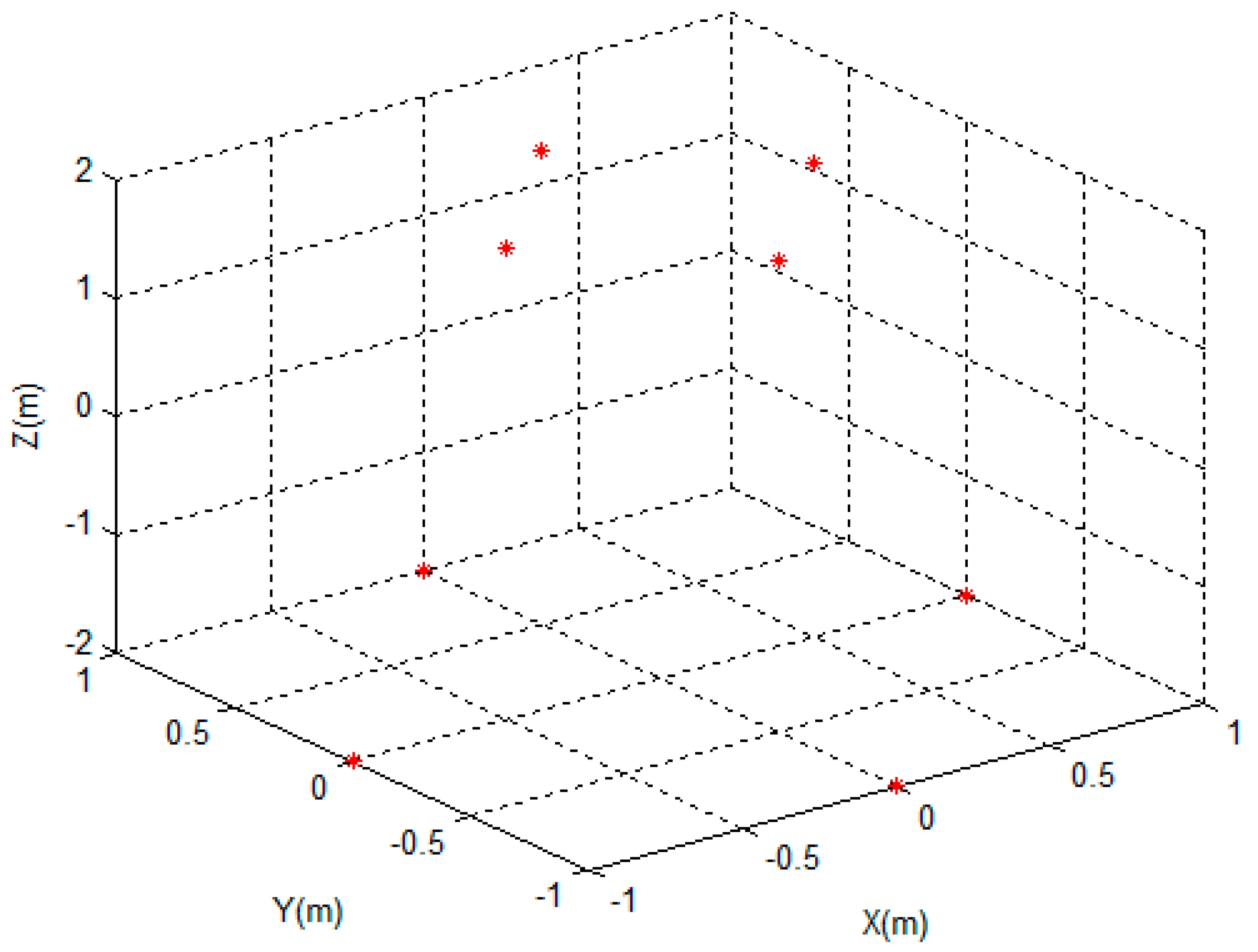
| Scattering Centre Index | X | Y | Z | Scattering Coefficient |
|---|---|---|---|---|
| #1 | 0.5 | 0 | 2 | 1 |
| #2 | −0.5 | 0 | 2 | 1 |
| #3 | 0 | 0.5 | 2 | 1 |
| #4 | 0 | −0.5 | 2 | 1 |
| #5 | 1.0 | 0 | −2 | 2 |
| #6 | −1.0 | 0 | −2 | 2 |
| #6 | 0 | 1.0 | −2 | 2 |
| #8 | 0 | −1.0 | −2 | 2 |
| Scattering Center Index | X | Y | Z |
|---|---|---|---|
| #1 | 0.5029 | −0.0030 | 1.9316 |
| #2 | −0.5024 | 0.0016 | 1.9324 |
| #3 | 0.0022 | 0.5023 | 1.9315 |
| #4 | 0.0024 | −0.5025 | 1.9317 |
| #5 | 1.0048 | 0.0029 | −1.9332 |
| #6 | −1.0048 | 0.0026 | −1.9316 |
| #6 | 0.0019 | 1.0052 | −1.9306 |
| #8 | 0.0025 | −1.0043 | −1.9323 |
© 2017 by the authors. Licensee MDPI, Basel, Switzerland. This article is an open access article distributed under the terms and conditions of the Creative Commons Attribution (CC BY) license ( http://creativecommons.org/licenses/by/4.0/).
Share and Cite
Bi, Y.; Wei, S.; Wang, J.; Mao, S. 3D Imaging of Rapidly Spinning Space Targets Based on a Factorization Method. Sensors 2017, 17, 366. https://doi.org/10.3390/s17020366
Bi Y, Wei S, Wang J, Mao S. 3D Imaging of Rapidly Spinning Space Targets Based on a Factorization Method. Sensors. 2017; 17(2):366. https://doi.org/10.3390/s17020366
Chicago/Turabian StyleBi, Yanxian, Shaoming Wei, Jun Wang, and Shiyi Mao. 2017. "3D Imaging of Rapidly Spinning Space Targets Based on a Factorization Method" Sensors 17, no. 2: 366. https://doi.org/10.3390/s17020366