
Robust Grape Cluster Detection in a Vineyard by Combining the AdaBoost Framework and Multiple Color Components


Abstract
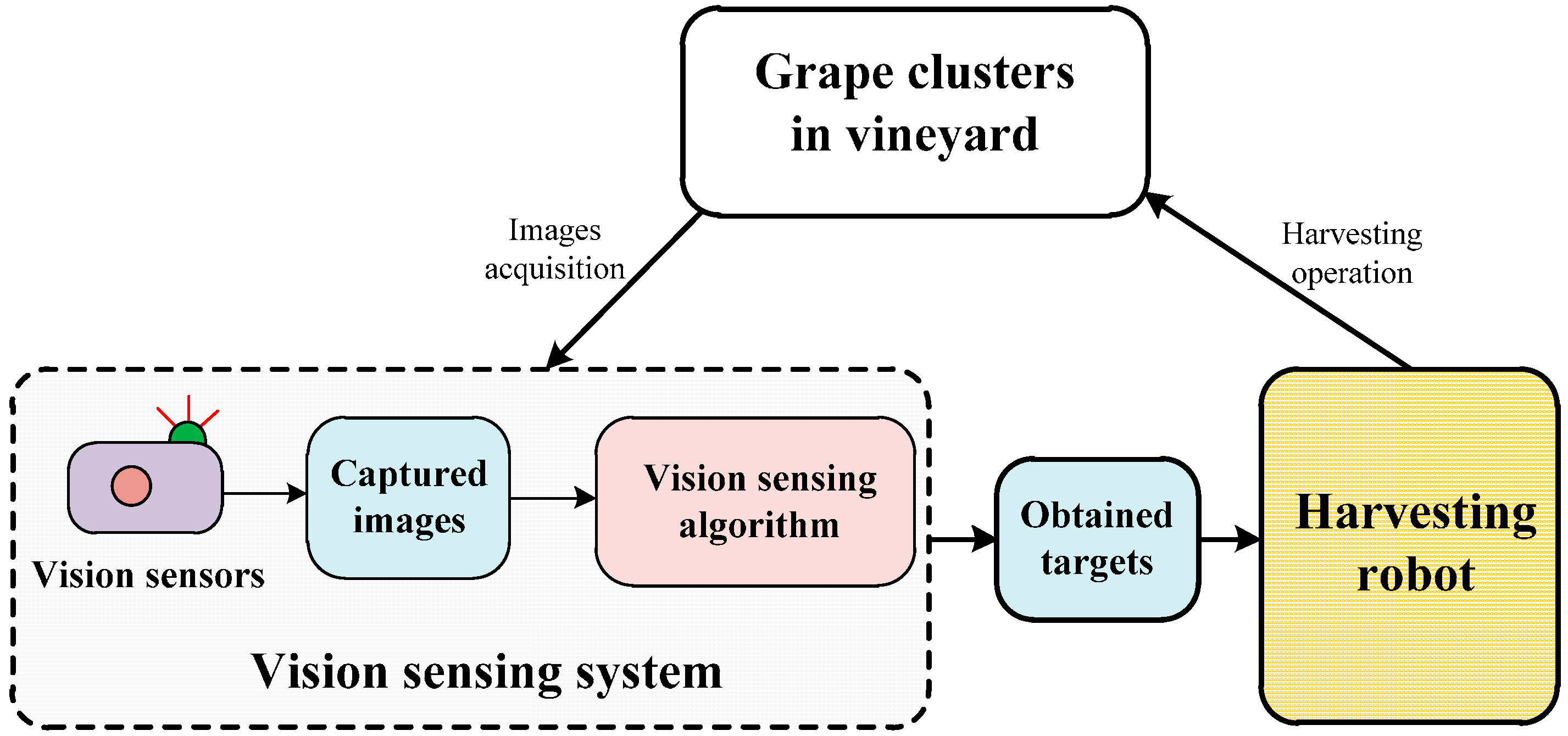
:1. Introduction
2. Materials and Methods
2.1. Image Acquisition and the Dataset
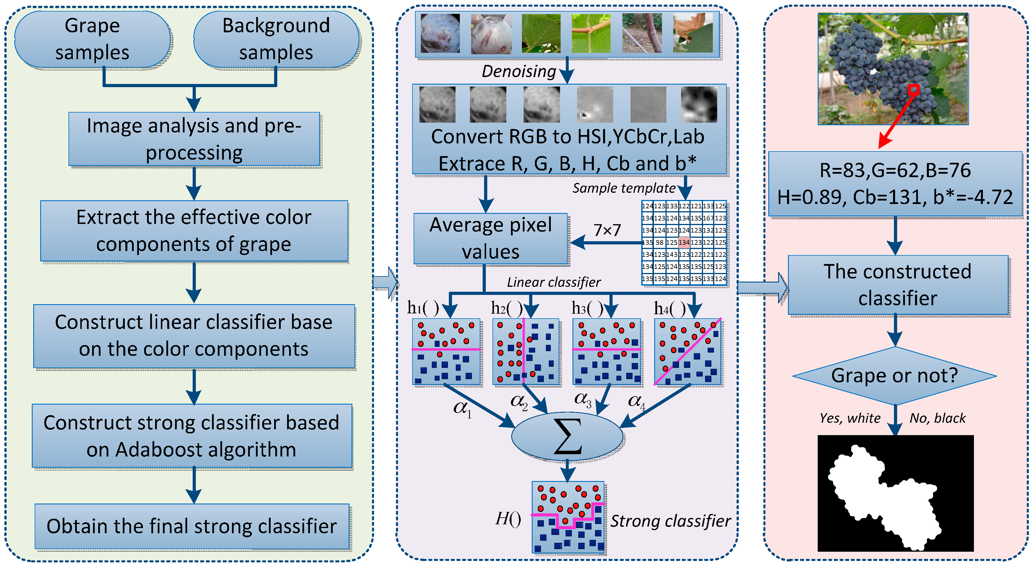
2.2. Detection Algorithm of Grape Clusters
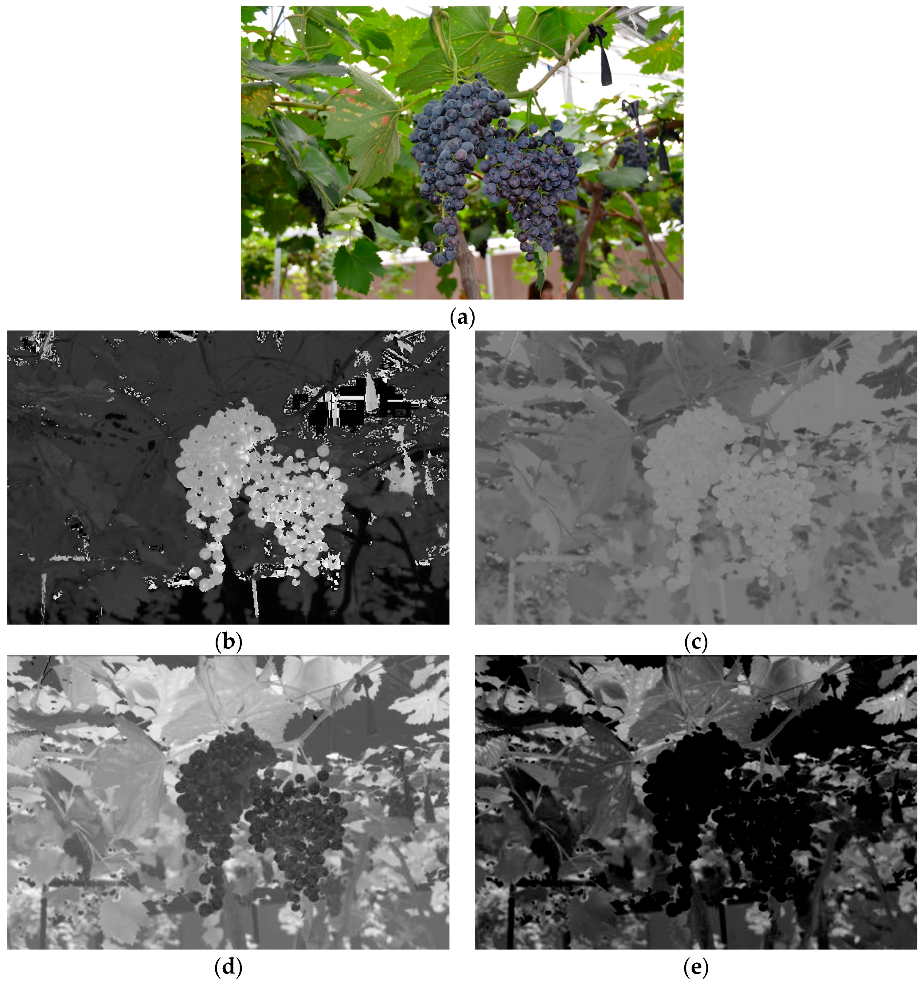
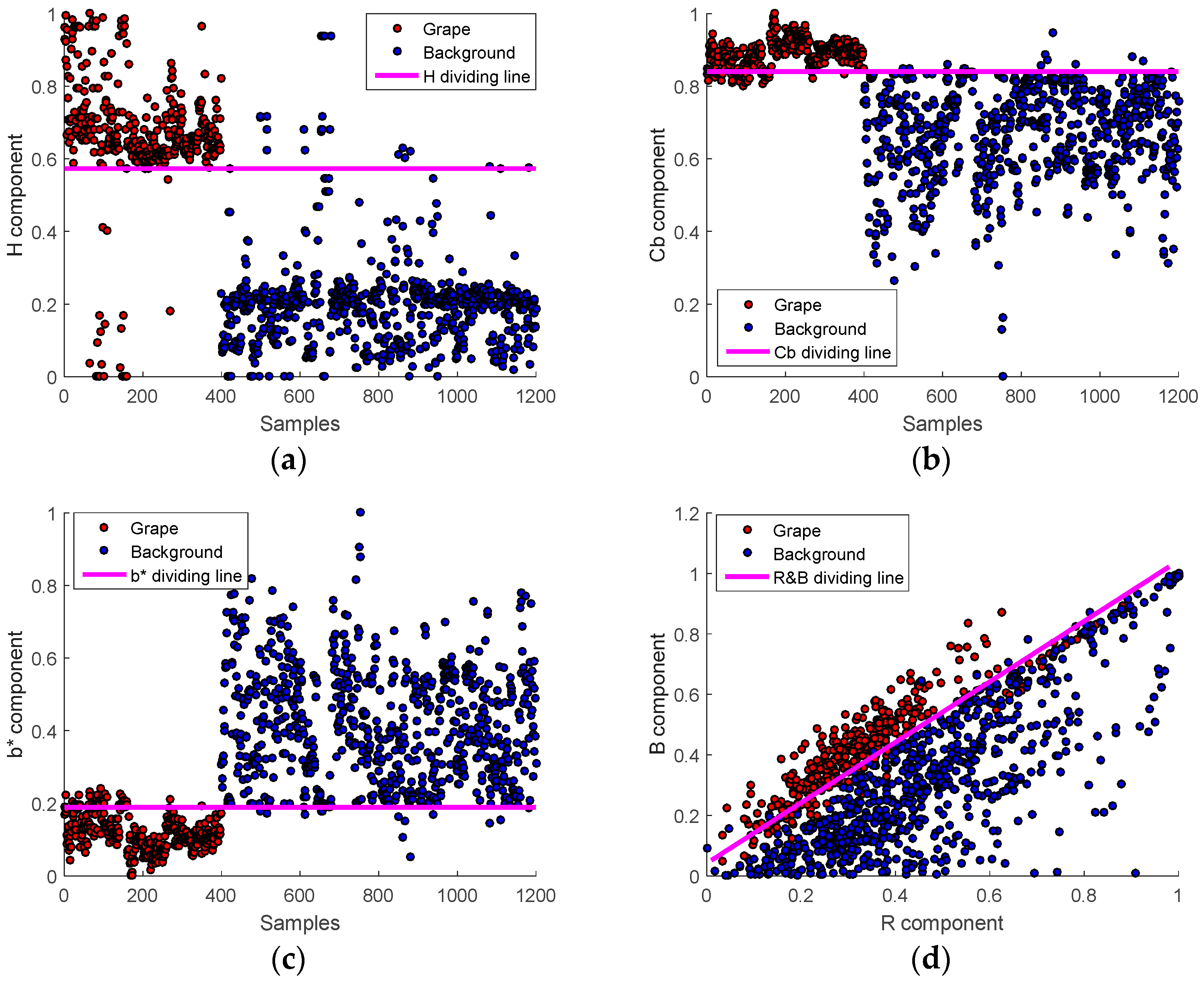
2.2.1. Color Analysis and Extraction of Multiple Effective Color Components
2.2.2. Construct Linear Classification Models Based on the Extracted Color Components
2.2.3. Construct Strong Classifier Based on the AdaBoost Framework
| Algorithm 1. The pseudo code of the constructed classifier. |
Input: Training samples set and number of learning rounds T.
% Train a learner from using based on the LCE method
|
| Output: The proposed classifier |
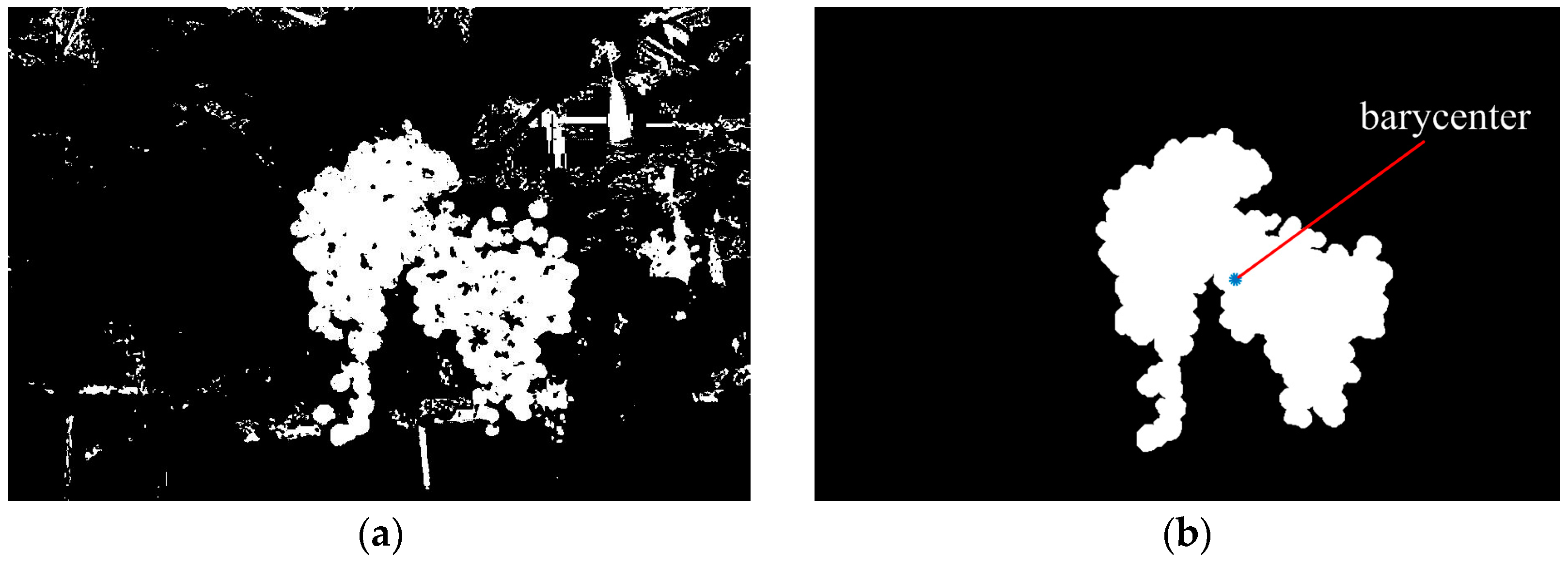
2.2.4. Images Pixels Classification and Targets Extraction
| Algorithm 2. The pseudo code of image segmentation and targets extraction. |
Input: Captured vineyard images
|
| Output: Binary image that contains only the grape clusters |
3. Experiments and Results
3.1. Accuracy of the Developed Classifier
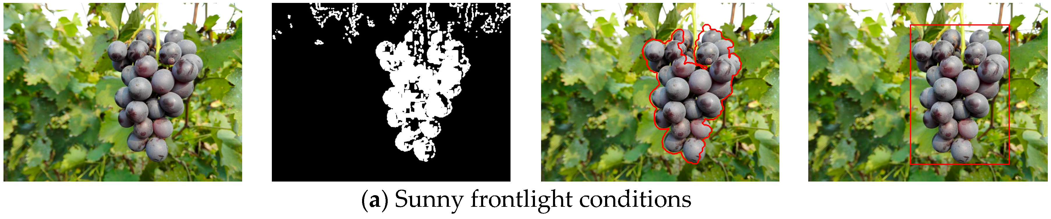
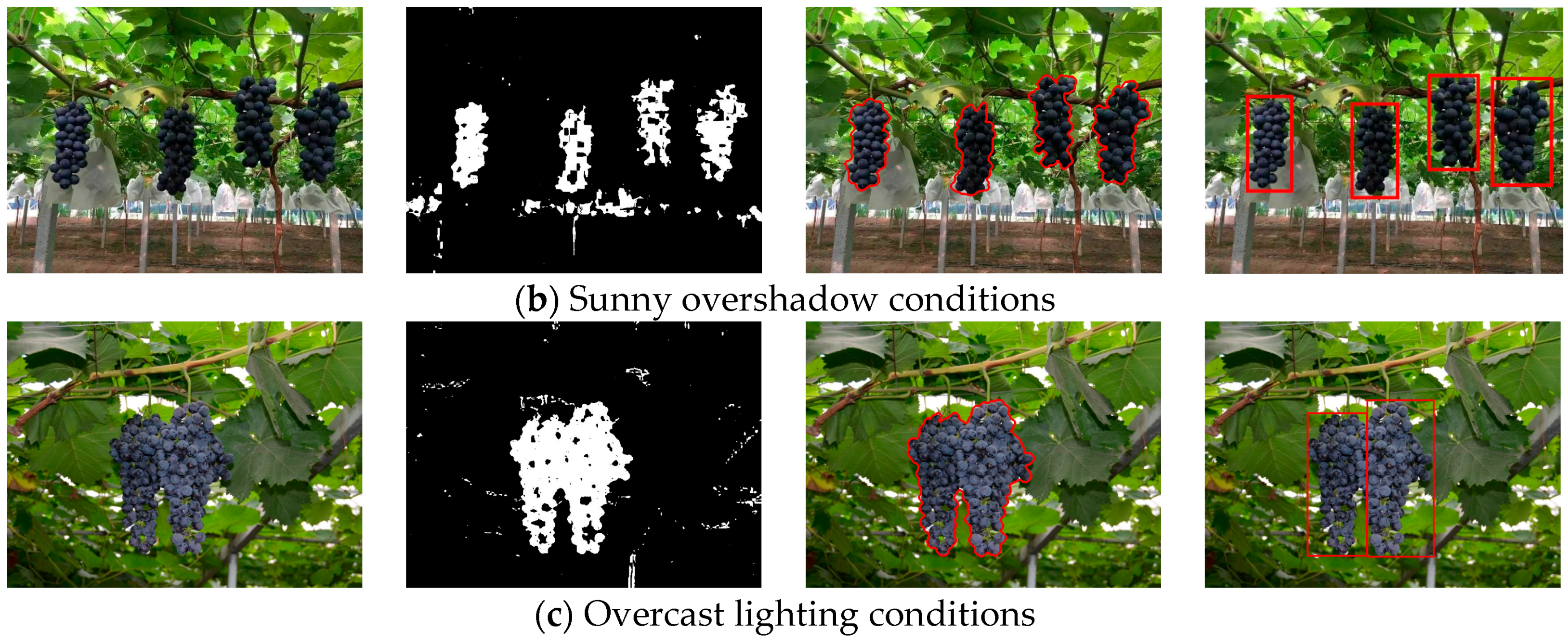
3.2. Detection of the Grape Clusters under Different Lighting Conditions
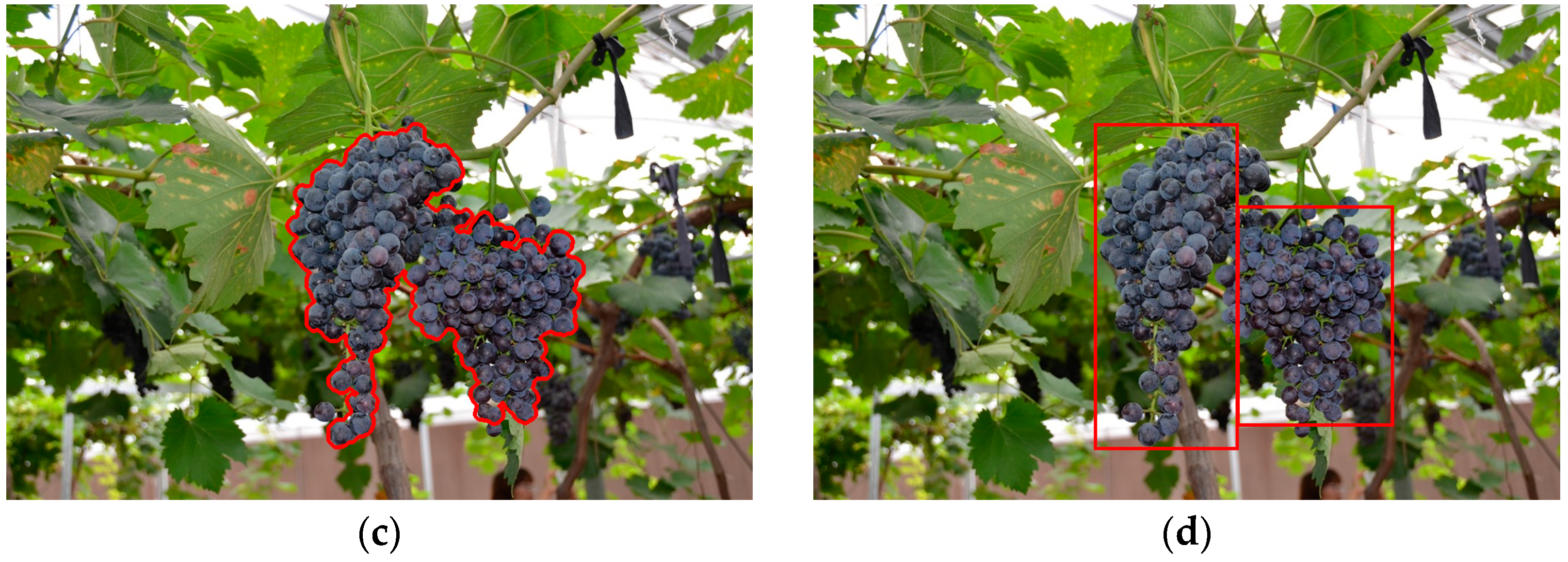
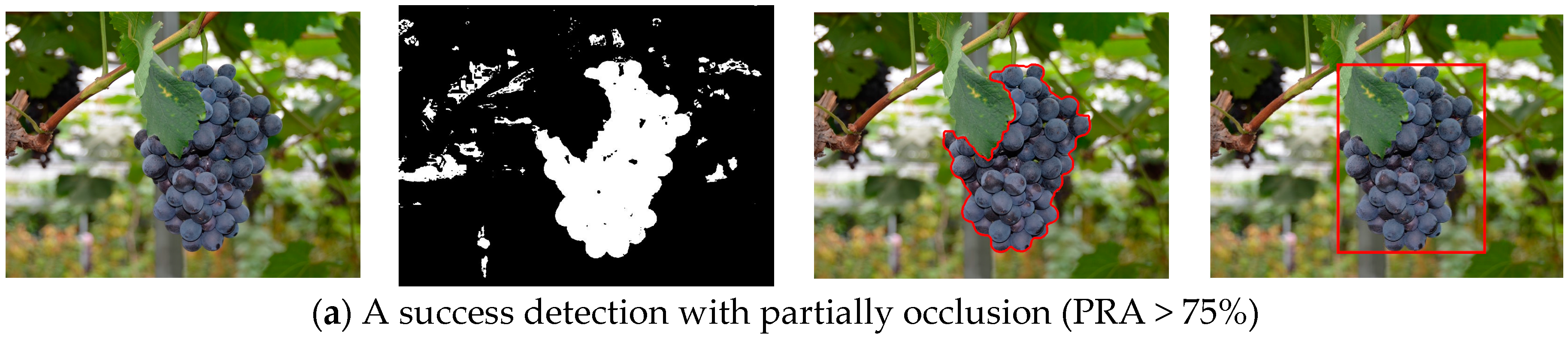
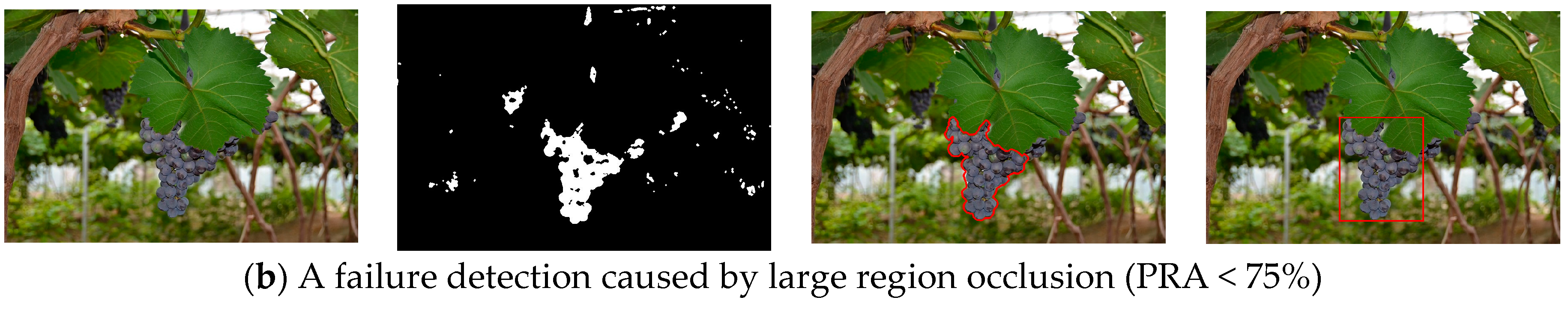
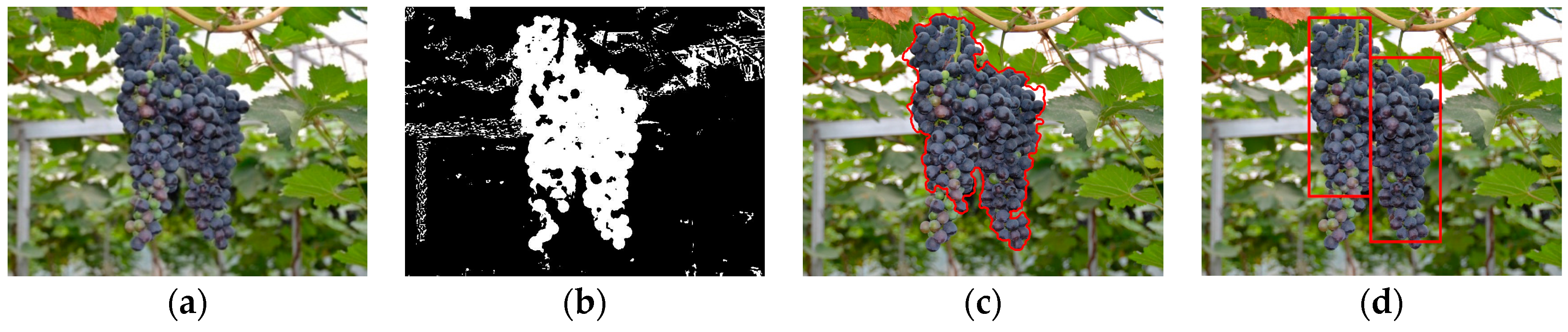
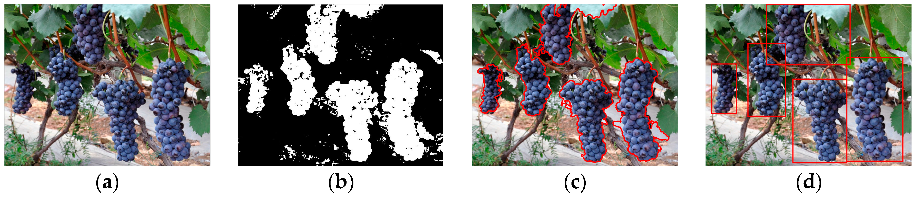
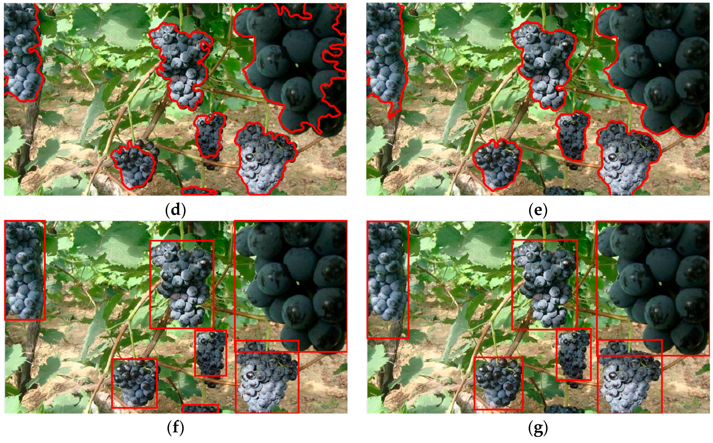
3.3. Performance of the Proposed Method against Adjacent and Occlusion Conditions
3.4. Comparing the Proposed Approach with Other Approach
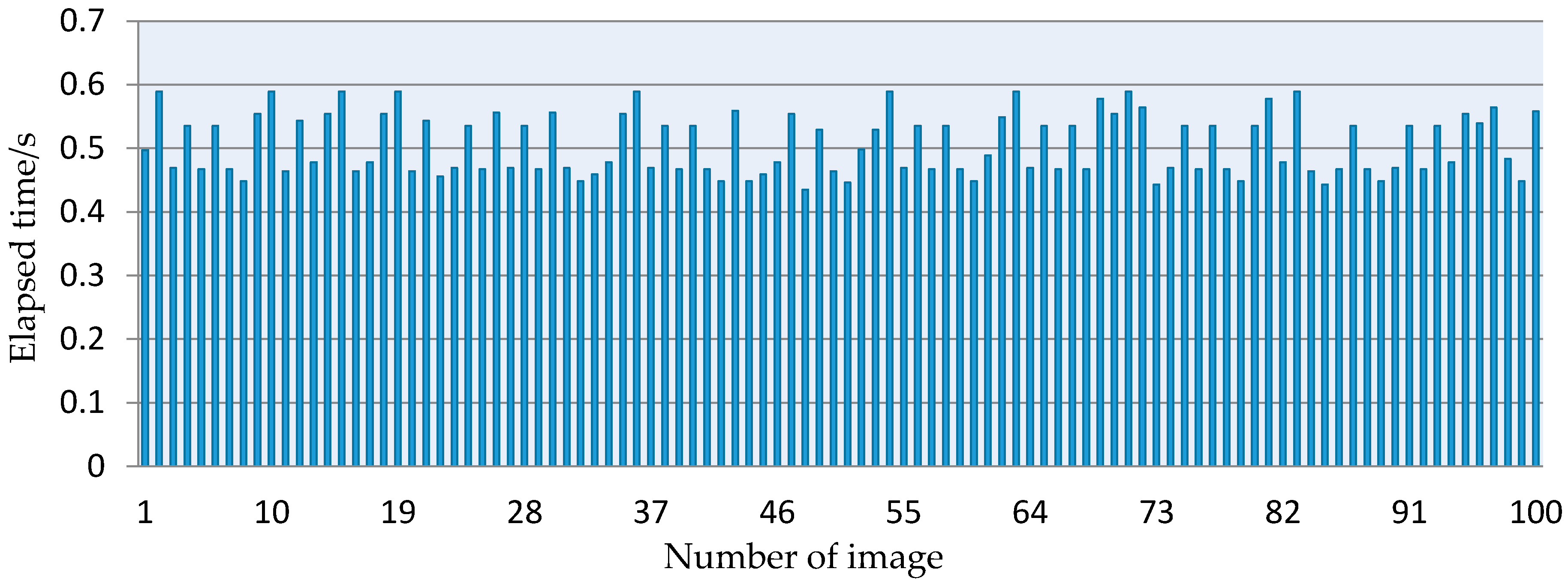
3.5. The Interactive Performance of the Developed Approach
4. Discussion
5. Conclusions and Future Work
- (1)
- The strong classifier was able to automatically distinguish the grapes from background, and the accuracy of the classifications can reach up to 96.56%, which was higher than with any weak classifier.
- (2)
- The success rate of the proposed detection algorithm was 93.74%, which was superior to other weak classifiers.
- (3)
- The interactive performance of the proposed detection algorithm was investigated, and the elapsed time of every image was less than 0.59 s, which can meet the requirements of harvesting robots.
Acknowledgments
Author Contributions
Conflicts of Interest
References
- Luo, L.; Tang, Y.; Zou, X.; Ye, M.; Feng, W.; Li, G. Vision-based extraction of spatial information in grape clusters for harvesting robots. Biosyst. Eng. 2016, 151, 90–104. [Google Scholar] [CrossRef]
- Gongal, A.; Amatya, S.; Karkee, M.; Zhang, Q.; Lewis, K. Sensors and systems for fruit detection and localization: A review. Comput. Electron. Agric. 2015, 116, 8–19. [Google Scholar] [CrossRef]
- Kondo, N.; Shibano, Y.; Mohri, K. Basic studies on robot to work in vineyard (Part 2). J. Jpn. Soc. Agric. Mach. 1994, 56, 45–53. [Google Scholar]
- Jimenez, A.R.; Ceres, R.; Pons, J.L. A vision system based on a laser range-finder applied to robotic fruit harvesting. Mach. Vis. Appl. 2000, 11, 321–329. [Google Scholar] [CrossRef]
- Wang, C.; Zou, X.; Tang, Y.; Luo, L.; Feng, W. Localisation of litchi in an unstructured environment using binocular stereo vision. Biosyst. Eng. 2016, 145, 39–51. [Google Scholar] [CrossRef]
- Font, D.; Pallejà, T.; Tresanchez, M.; Runcan, D.; Moreno, J.; Martínez, D.; Teixidó, M.; Palacín, J. A proposal for automatic fruit harvesting by combining a low cost stereovision camera and a robotic arm. Sensors 2014, 14, 11557–11579. [Google Scholar] [CrossRef] [PubMed]
- Feng, J.; Zeng, L.; Liu, G. Fruit recognition algorithm based on multi-source images fusion. Trans. CSAM 2014, 45, 73–80. [Google Scholar]
- Zhao, Y.; Gong, L.; Zhou, B.; Huang, Y.; Liu, C. Detecting tomatoes in greenhouse scenes by combining AdaBoost classifier and colour analysis. Biosyst. Eng. 2016, 148, 127–137. [Google Scholar] [CrossRef]
- Berenstein, R.; Ben Shahar, O.; Shapiro, A.; Edan, Y. Grape clusters and foliage detection algorithms for autonomous selective vineyard sprayer. Intell. Serv. Robot. 2010, 3, 233–243. [Google Scholar] [CrossRef]
- Font, D.; Pallejà, T.; Tresanchez, M.; Teixidó, M.; Martinez, D. Counting red grapes in vineyards by detecting specular spherical reflection peaks in RGB images obtained at night with artificial illumination. Comput. Electron. Agric. 2014, 108, 105–111. [Google Scholar] [CrossRef]
- Reis, M.J.C.S.; Morais, R.; Peres, E.; Pereira, C.; Contente, O.; Soares, S.; Valente, A.; Baptista, J.; Ferreira, P.J.S.G.; Bulas Cruz, J. Automatic detection of bunches of grapes in natural environment from color images. J. App. Log. 2012, 10, 285–290. [Google Scholar] [CrossRef]
- Luo, L.; Zou, X.; Yang, Z.; Li, G.; Song, X.; Zhang, C. Grape image fast segmentation based on improved artificial bee colony and fuzzy clustering. Trans. CSAM 2015, 46, 23–28. [Google Scholar]
- Fu, L.S.; Wang, B.; Cui, Y.J.; Su, S.; Gejima, Y.; Kobayashi, T. Kiwifruit recognition at nighttime using artificial lighting based on machine vision. Int. J. Agric. Biol. Eng. 2015, 8, 52–59. [Google Scholar]
- Font, D.; Tresanchez, M.; Martínez, D.; Moreno, J.; Clotet, E.; Palacín, J. Vineyard Yield Estimation Based on the Analysis of High Resolution Images Obtained with Artificial Illumination at Night. Sensors 2015, 15, 8284–8301. [Google Scholar] [CrossRef] [PubMed]
- Slaughter, D.C.; Harrel, R.C. Color vision in robotic fruit harvesting. Trans. ASAE 1987, 30, 1144–1148. [Google Scholar] [CrossRef]
- Cheng, H.D.; Jiang, X.H.; Sun, Y.; Wang, J. Color image segmentation: Advances and prospects. Pattern Recognit. 2001, 34, 2259–2281. [Google Scholar] [CrossRef]
- Teixidó, M.; Font, D.; Pallejà, T.; Tresanchez, M.; Nogués, M.; Palacín, J. Definition of linear color models in the RGB vector color space to detect red peaches in orchard images taken under natural illumination. Sensors 2012, 12, 7701–7718. [Google Scholar] [CrossRef] [PubMed]
- Liu, S.; Whitty, M. Automatic grape bunch detection in vineyards with an SVM classifier. J. Appl. Log. 2015, 13, 643–653. [Google Scholar] [CrossRef]
- Nuske, S.; Achar, S.; Bates, T.; Narasimhan, S.; Singh, S. Yield estimation in vineyards by visual grape detection. In Proceedings of the IEEE/RSJ International Conference on Intelligent Robots and Systems, San Francisco, CA, USA, 25–30 September 2011; pp. 2352–2358.
- Diago, M.P.; Correa, C.; Millán, B.; Barreiro, P.; Valero, C.; Tardaguila, J. Grapevine yield and leaf area estimation using supervised classification methodology on RGB images taken under field conditions. Sensors 2012, 12, 16988–17006. [Google Scholar] [CrossRef] [PubMed] [Green Version]
- Wei, X.; Jia, K.; Lan, J.; Li, Y.; Zeng, Y.; Wang, C. Automatic method of fruit object extraction under complex agricultural background for vision system of fruit picking robot. Optik 2014, 125, 5684–5689. [Google Scholar] [CrossRef]
- Yamamoto, K.; Guo, W.; Yoshioka, Y.; Ninomiya, S. On plant detection of intact tomato fruits using image analysis and machine learning methods. Sensors 2014, 14, 12191–12206. [Google Scholar] [CrossRef] [PubMed]
- Chamelat, R.; Rosso, E.; Choksuriwong, A.; Rosenberger, C. Grape detection by image processing. In Proceedings of the 32nd Annual Conference on IEEE Industrial Electronics, Paris, France, 6–10 November 2006; pp. 3697–3702.
- Zhu, Y.; Cao, Z.; Lu, H.; Li, Y.; Xiao, Y. In-field automatic observation of wheat heading stage using computer vision. Biosyst. Eng. 2016, 143, 28–41. [Google Scholar] [CrossRef]
- Kong, K.K.; Hong, K.S. Design of coupled strong classifiers in AdaBoost framework and its application to pedestrian detection. Pattern Recognit. Lett. 2015, 68, 63–69. [Google Scholar] [CrossRef]
- Kicherer, A.; Herzog, K.; Pflanz, M.; Wieland, M.; Rüger, P.; Kecke, S.; Kuhlmann, H.; Töpfer, R. An automated field phenotyping pipeline for application in grapevine research. Sensors 2015, 15, 4823–4836. [Google Scholar] [CrossRef] [PubMed]
- Kotsiantis, S.B. Supervised machine learning: A review of classification techniques. Informatica 2007, 31, 249–268. [Google Scholar]
- Zhou, Z. Ensemble Learning; Springer: Berlin, Germany, 2008. [Google Scholar]
- Freund, Y.; Schapire, R.E. A short introduction to boosting. J. Jpn. Soc. Artif. Intell. 1999, 14, 771–780. [Google Scholar]
- Si, Y.; Liu, G.; Feng, J. Location of apples in trees using stereoscopic vision. Comput. Electron. Agric. 2015, 112, 68–74. [Google Scholar] [CrossRef]
- Kenneth, R.C. Digital Image Processing; Prentice Hall: Upper Saddle River, NJ, USA, 1996. [Google Scholar]
- Gonzalez, R.C.; Woods, R.E.; Eddins, S.L. Digital Image Processing Using MATLAB; Publish House of Ecectronics Industry: Beijing, China, 2012; pp. 152–158. [Google Scholar]
- Smitii, T.; Guild, J. The C.I.E colorimetric standards and their use. Trans. Opt. Soc. 1932, 3, 73–134. [Google Scholar] [CrossRef]
- Freund, Y.; Schapire, R.E. A decision-theoretic generalization of on-line leaning and an application to Booting. J. Comput. Syst. Sci. 1997, 55, 119–139. [Google Scholar] [CrossRef]
- Freund, Y.; Schapire, R.E. Experiments with a New Boosting Algorithm. In Proceedings of the 13th International Conference on Machine Learning, Bari, Italy, 3–6 July 1996; Morgan Kaufmann: San Francisco, CA, USA, 1996; pp. 148–156. [Google Scholar]
- Zhang, C.; Zhang, J.; Zhang, G. An efficient modified boosting method for solving classification problems. J. Comput. Appl. Math. 2008, 214, 381–392. [Google Scholar] [CrossRef]
- Jakkrit, T.; Cholwich, N.; Thanaruk, T. Boosting-based ensemble learning with penalty profiles for automatic Thai unknown word recognition. Comput. Math. Appl. 2012, 63, 1117–1134. [Google Scholar]
- Park, K.Y.; Hwang, S.Y. An improved Haar-like feature for efficient object detection. Pattern Recognit. Lett. 2014, 42, 148–153. [Google Scholar] [CrossRef]
- Zou, X.; Ye, M.; Luo, C.; Xiong, T.; Luo, L.; Chen, Y.; Wang, H. Fault-tolerant design of a limited universal fruit-picking end-effector based on visoin positioning error. Appl. Eng. Agric. 2016, 32, 5–18. [Google Scholar]


| Classifiers | Classifiers of Equation | Errors/ | Weight of Weak Classifiers/ |
|---|---|---|---|
| H() − 0.57 = 0 | 0.044 | 1.537 | |
| Cb() − 0.86 = 0 | 0.119 | 1.001 | |
| 0.31 − Lab_b() = 0 | 0.225 | 0.620 | |
| 10×B() − 6.16×R() − 1.3 = 0 | 0.341 | 0.331 | |
| Classifiers | Actual Categories | Samples Number | Classified Categories | /% | /% | |
|---|---|---|---|---|---|---|
| Grape | Background | |||||
| Grape | 300 | 276 | 24 | 93.67 | 6.33 | |
| Background | 600 | 33 | 567 | |||
| Grape | 300 | 231 | 69 | 90.22 | 9.78 | |
| Background | 600 | 19 | 581 | |||
| Grape | 300 | 259 | 41 | 81.33 | 18.67 | |
| Background | 600 | 127 | 473 | |||
| Grape | 300 | 278 | 22 | 83.56 | 16.44 | |
| Background | 600 | 126 | 474 | |||
| Grape | 300 | 282 | 18 | 96.56 | 3.44 | |
| Background | 600 | 13 | 587 | |||
| Lighting Conditions | Grape Clusters | True Positives | False Negatives | False Positives | |||
|---|---|---|---|---|---|---|---|
| Amount | /% | Amount | /% | Amount | /% | ||
| Sunny frontlight | 136 | 128 | 94.12 | 5 | 3.76 | 8 | 5.88 |
| Sunny overshadow | 129 | 118 | 91.47 | 6 | 4.84 | 11 | 8.53 |
| Overcast lighting | 182 | 173 | 95.05 | 8 | 4.42 | 9 | 4.95 |
| Total | 447 | 419 | 93.74 | 19 | 4.34 | 28 | 6.26 |
| Sequence Number of Grape Clusters | The RPA of Paper [18]/% | The RPA of the Proposed Method/% |
|---|---|---|
| 1 | 91.27 | 93.43 |
| 2 | 86.82 | 92.86 |
| 3 | 88.76 | 93.73 |
| 4 | 90.57 | 89.23 |
| 5 | 91.75 | 89.75 |
| 6 | 90.26 | 91.26 |
| 7 | 92.27 | 95.23 |
| 8 | 89.78 | 88.95 |
| 9 | 86.53 | 89.26 |
| 10 | 87.36 | 91.23 |
| 11 | 89.26 | 93.69 |
| 12 | 93.45 | 92.26 |
| 13 | 88.36 | 87.63 |
| 14 | 91.59 | 94.45 |
| Average value | 89.86 | 91.49 |
© 2016 by the authors; licensee MDPI, Basel, Switzerland. This article is an open access article distributed under the terms and conditions of the Creative Commons Attribution (CC-BY) license (http://creativecommons.org/licenses/by/4.0/).
Share and Cite
Luo, L.; Tang, Y.; Zou, X.; Wang, C.; Zhang, P.; Feng, W. Robust Grape Cluster Detection in a Vineyard by Combining the AdaBoost Framework and Multiple Color Components. Sensors 2016, 16, 2098. https://doi.org/10.3390/s16122098
Luo L, Tang Y, Zou X, Wang C, Zhang P, Feng W. Robust Grape Cluster Detection in a Vineyard by Combining the AdaBoost Framework and Multiple Color Components. Sensors. 2016; 16(12):2098. https://doi.org/10.3390/s16122098
Chicago/Turabian StyleLuo, Lufeng, Yunchao Tang, Xiangjun Zou, Chenglin Wang, Po Zhang, and Wenxian Feng. 2016. "Robust Grape Cluster Detection in a Vineyard by Combining the AdaBoost Framework and Multiple Color Components" Sensors 16, no. 12: 2098. https://doi.org/10.3390/s16122098