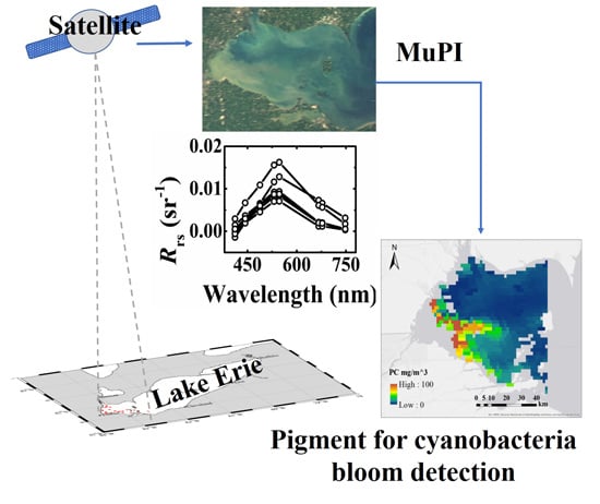
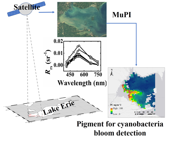
Multi-Spectral Remote Sensing of Phytoplankton Pigment Absorption Properties in Cyanobacteria Bloom Waters: A Regional Example in the Western Basin of Lake Erie


Abstract
:
1. Introduction
2. Materials and Methods
2.1. In Situ Measurements
2.1.1. Study Areas
2.1.2. Remote Sensing Reflectance
2.1.3. Absorption Coefficients
2.1.4. Pigment Concentrations and Group Composition
2.2. Satellite Imagery
2.3. The aGau(λ) Estimation
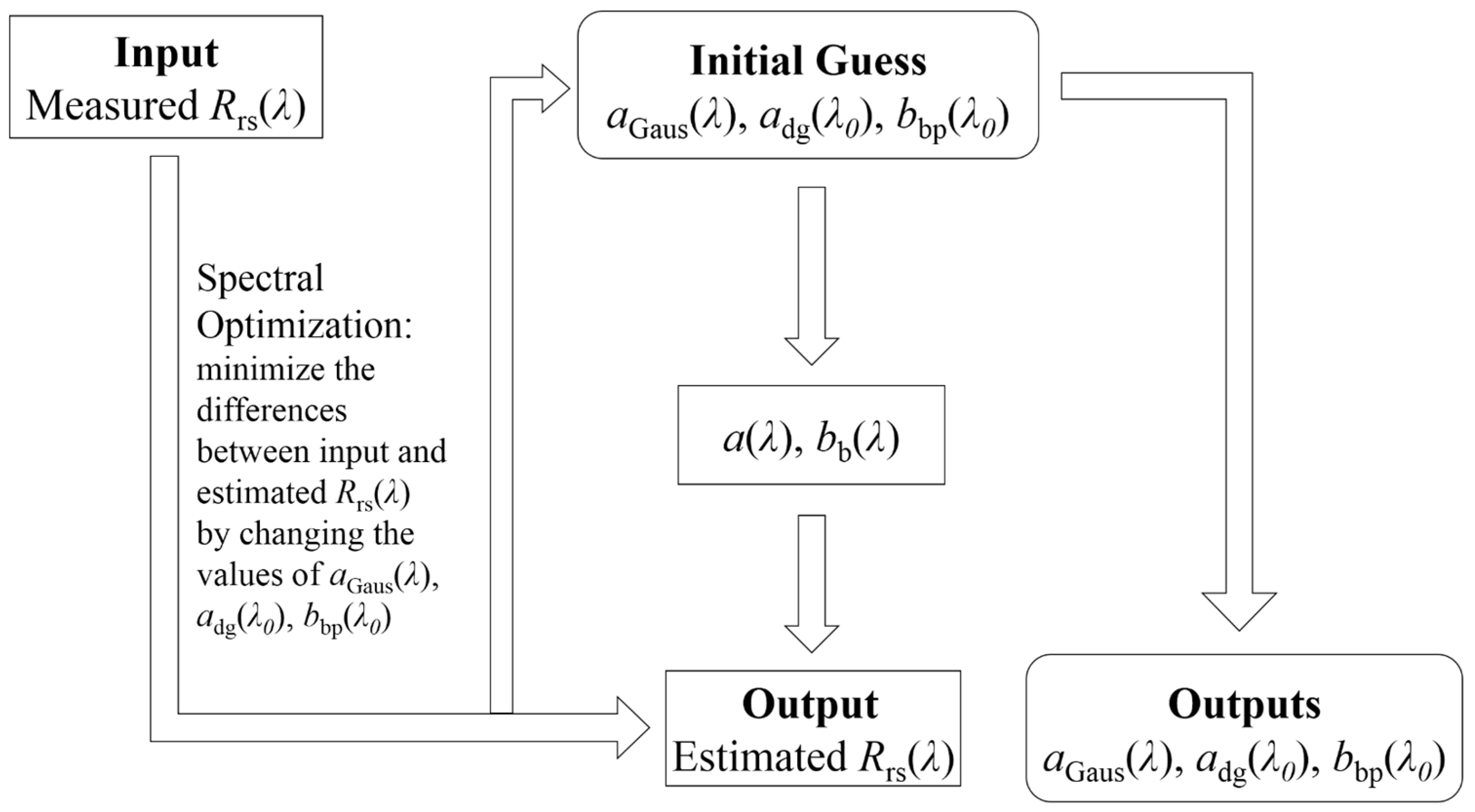
2.3.1. MuPI Model
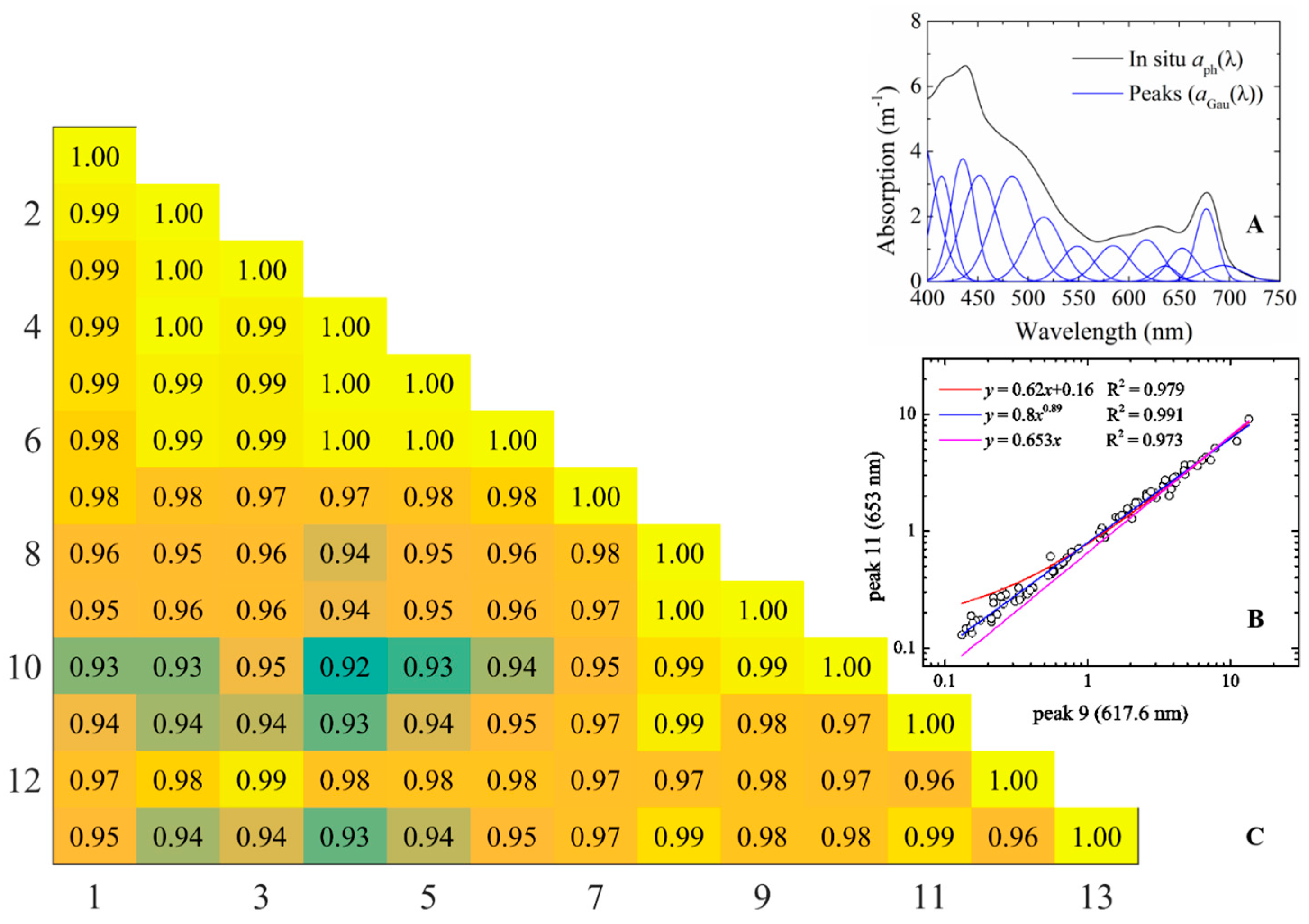
2.3.2. Gaussian Parameters
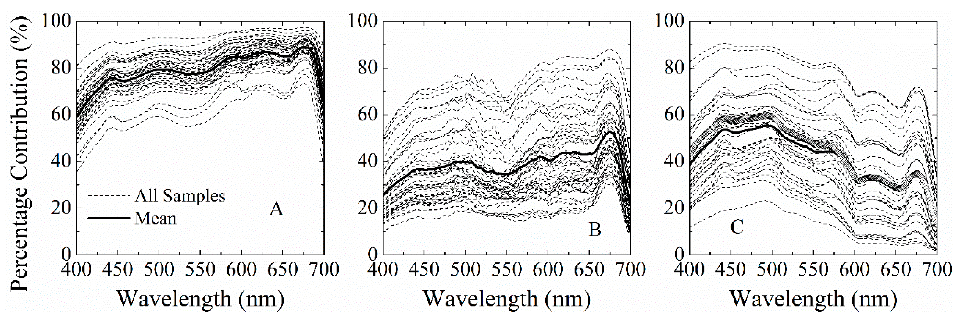
2.4. aGau(λ) Spectra Shape
2.5. Multi-Spectral Rrs(λ)
3. Results
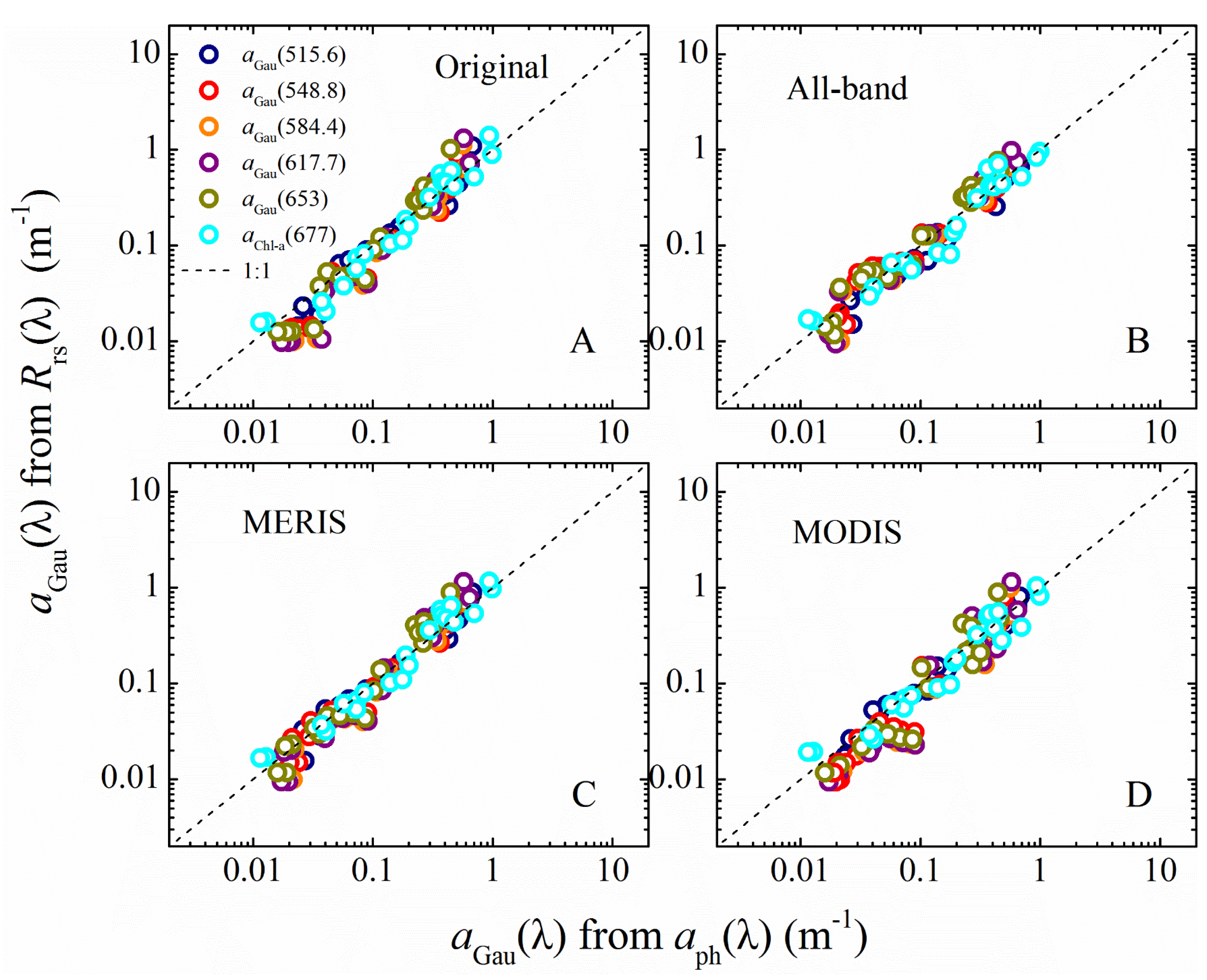
3.1. aGau(λ) from Multi-Spectral Rrs(λ)
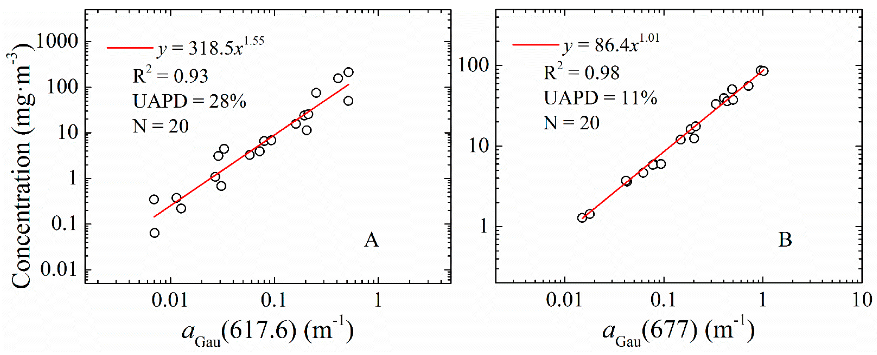
3.2. Chl-a and PC from aGau(λ) for Lake Erie
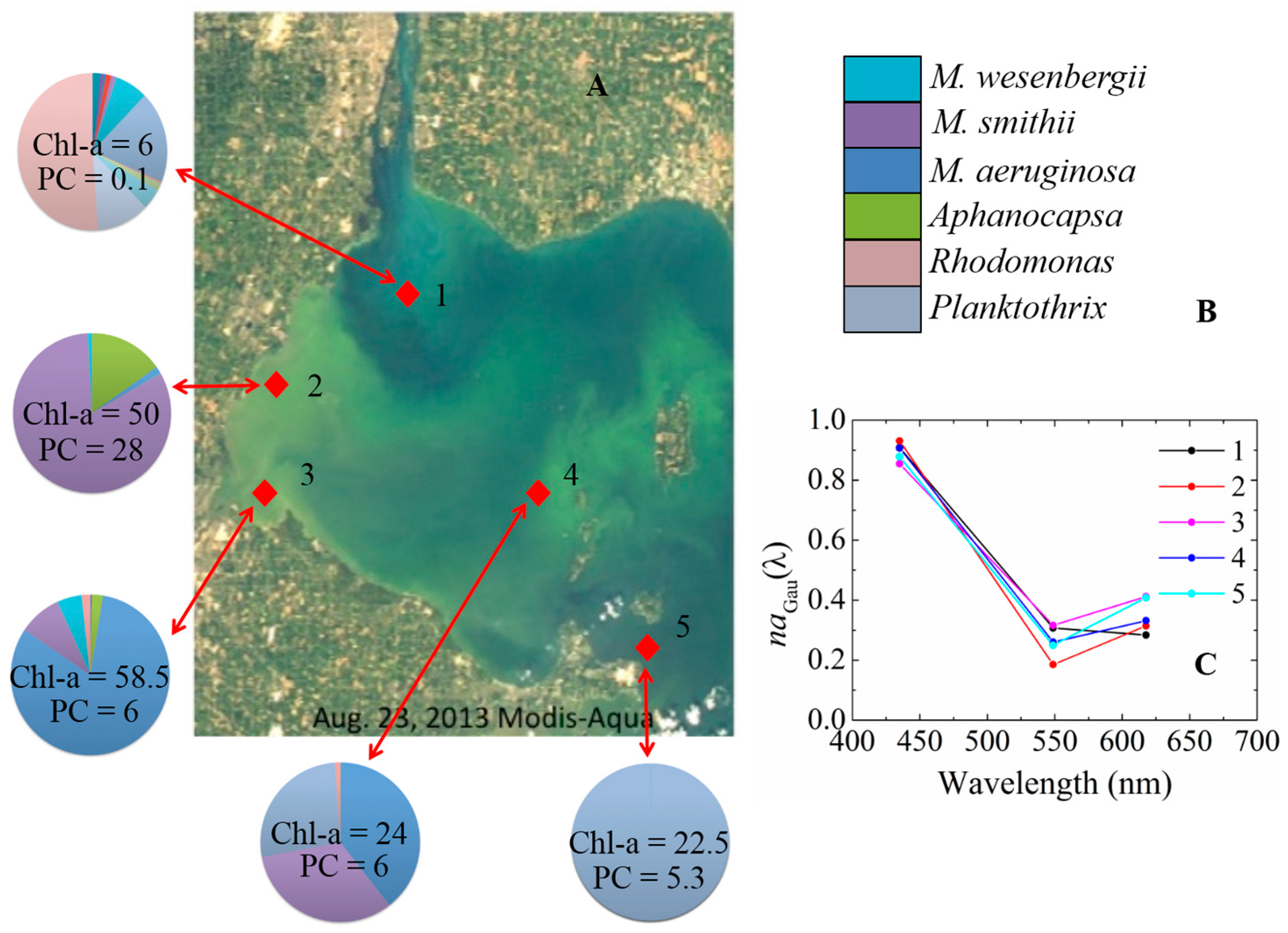
3.3. aGau(λ) versus Group Composition
3.4. Pigment and aGau(λ) Retrieval from Satellite Imagery
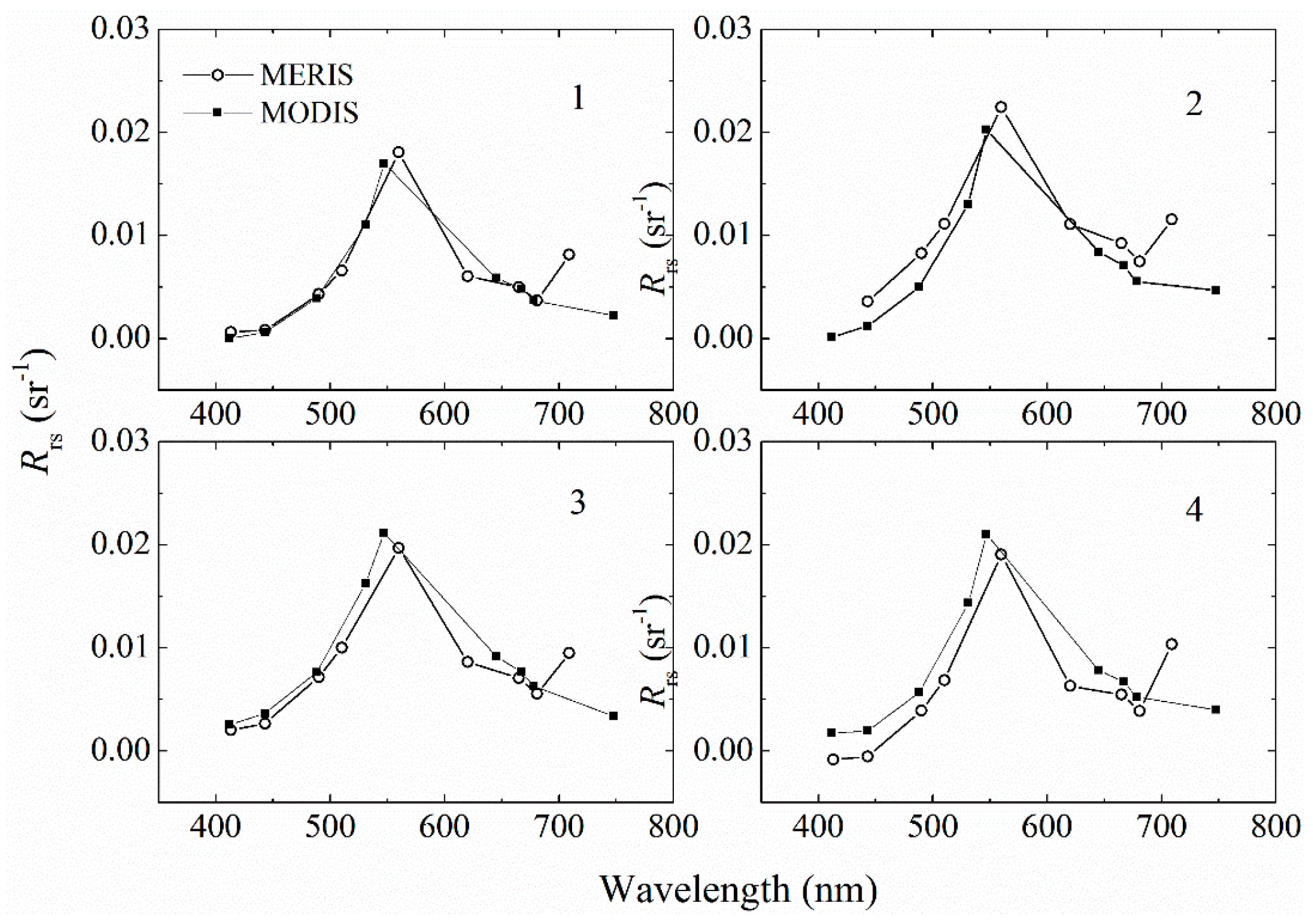
3.4.1. Validation of Satellite Remote Sensing Data
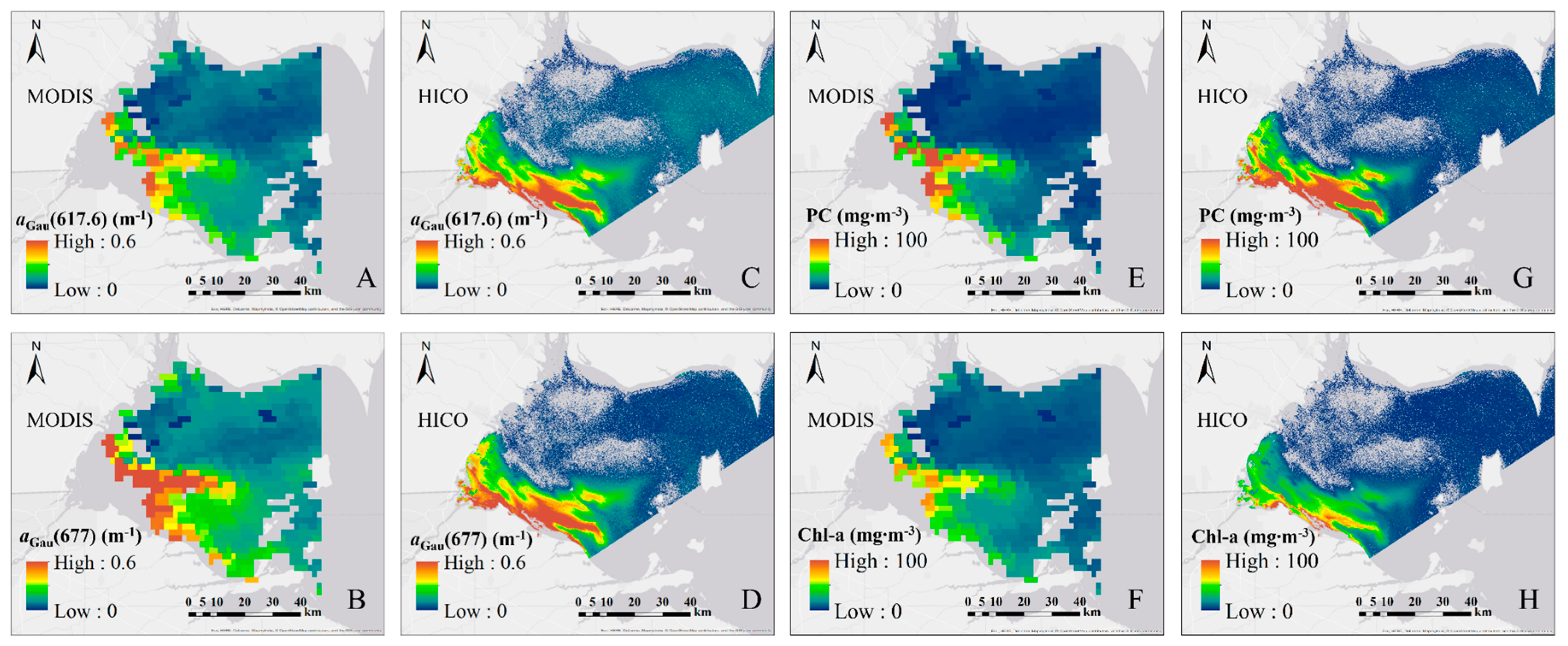
3.4.2. Chl-a and PC from HICO and MODIS Imagery
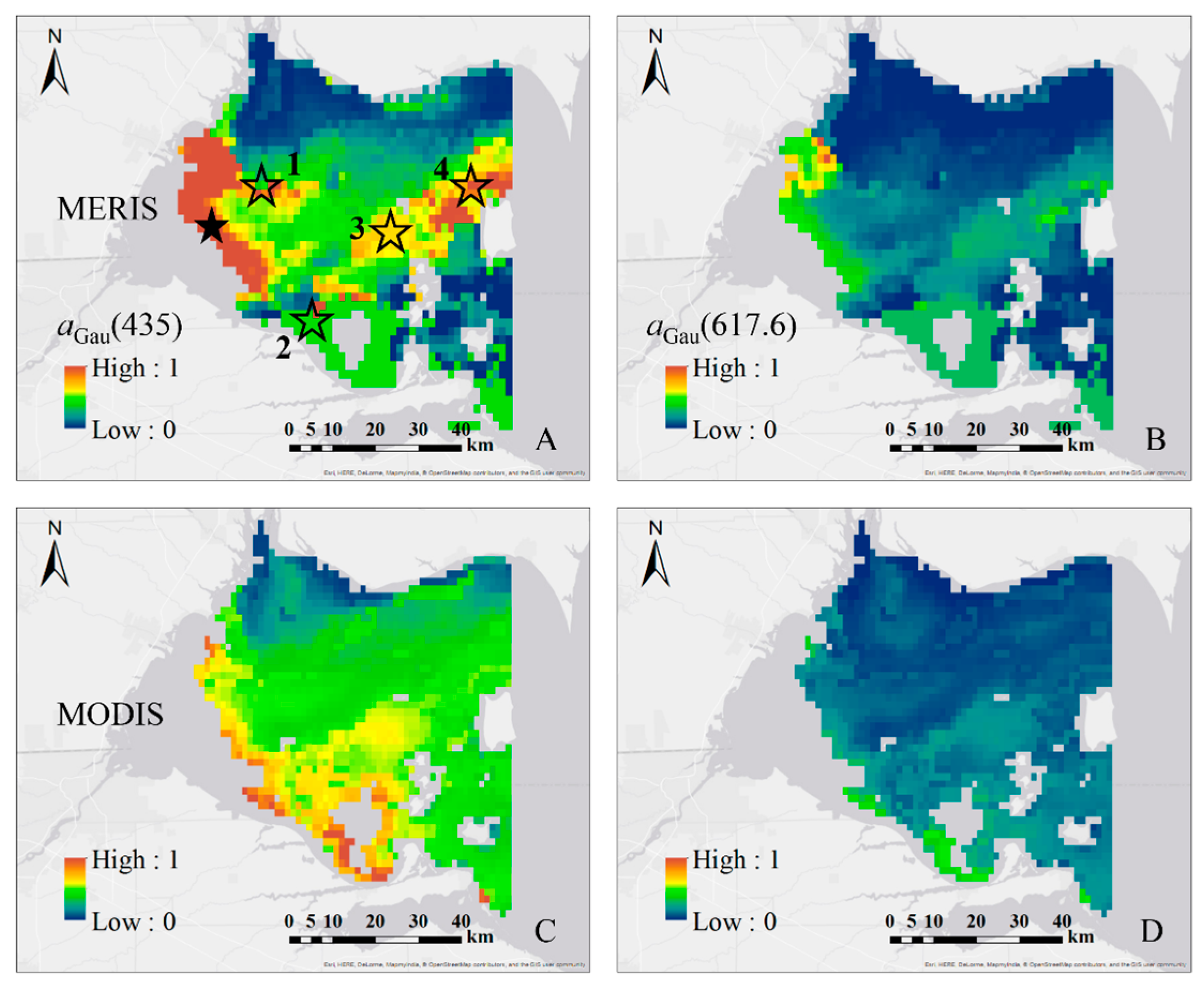
3.4.3. MODIS and MERIS Imagery over Lake Erie
3.4.4. The Seasonal Variation of aGau(λ) from MERIS Imagery
4. Discussion
4.1. Spectral Requirements for aGau(λ) Retrieval
4.2. The seasonal aGau(λ) Variation in Lake Erie
4.3. Pigment Retrieval and HABs Detection
5. Conclusions
Supplementary Materials
Acknowledgments
Author Contributions
Conflicts of Interest
References
- Jeffrey, S.W.; Mantoura, R.F.C.; Wright, S.W. Phytoplankton Pigments in Oceanography: Guidelines to Modern Methods (Monographs on Oceanographic Methodology); UNESCO Publishing: Paris, France, 1997; p. 661. [Google Scholar]
- Sosik, H.M.; Mitchell, B.G. Light absorption by phytoplankton, photosynthetic pigments and detritus in the California Current System. Deep Sea Res. Part I 1995, 42, 1717–1748. [Google Scholar] [CrossRef]
- Schlüter, L.; Møhlenberg, F.; Havskum, H.; Larsen, S. The use of phytoplankton pigments for identifying and quantifying phytoplankton groups in coastal areas: Testing the influence of light and nutrients on pigment/chlorophyll a ratios. Mar. Ecol. Prog. Ser. 2000, 192, 49–63. [Google Scholar] [CrossRef]
- The International Ocean-Colour Coordinating Group (IOCCG). Phytoplankton Functional Types from Space; Sathyendranath, S., Ed.; Reports of the International Ocean-Colour Coordinating Group, No. 15; IOCCG: Dartmouth, NS, Canada, 2014. [Google Scholar]
- Mouw, C.B.; Hardman-Mountford, N.J.; Alvain, S.; Bracher, A.; Brewin, R.J.W.; Bricaud, A.; Ciotti, A.M.; Devred, E.; Fujiwara, A.; Hirata, T.; et al. A Consumer’s Guide to Satellite Remote Sensing of Multiple Phytoplankton Groups in the Global Ocean. Front. Mar. Sci. 2017, 4. [Google Scholar] [CrossRef]
- Simis, S.G.; Peters, S.W.; Gons, H.J. Remote sensing of the cyanobacterial pigment phycocyanin in turbid inland water. Limnol. Oceanogr. 2005, 50, 237–245. [Google Scholar] [CrossRef]
- Wynne, T.T.; Stumpf, R.P.; Tomlinson, M.C.; Warner, R.A.; Tester, P.A.; Dyble, J.; Fahnenstiel, G.L. Relating spectral shape to cyanobacterial blooms in the Laurentian Great Lakes. Int. J. Remote Sens. 2008, 29, 3665–3672. [Google Scholar] [CrossRef]
- Pan, X.; Mannino, A.; Russ, M.E.; Hooker, S.B.; Harding, L.W. Remote sensing of phytoplankton pigment distribution in the United States northeast coast. Remote Sens. Environ. 2010, 114, 2403–2416. [Google Scholar] [CrossRef]
- Wang, G.; Lee, Z.; Mishra, D.R.; Ma, R. Retrieving absorption coefficients of multiple phytoplankton pigments from hyperspectral remote sensing reflectance measured over cyanobacteria bloom waters. Limnol. Oceanogr. Methods 2016, 14, 432–447. [Google Scholar] [CrossRef]
- Hoepffner, N.; Sathyendranath, S. Effect of pigment composition on absorption properties of phytoplankton. Mar. Ecol. Prog. Ser. 1991, 73, 11–23. [Google Scholar] [CrossRef]
- Hoepffner, N.; Sathyendranath, S. Determination of the major groups of phytoplankton pigments from the absorption spectra of total particulate matter. J. Geophys. Res. 1993, 98, 22789–22803. [Google Scholar] [CrossRef]
- Bidigare, R.R.; Morrow, J.H.; Kiefer, D.A. Derivative analysis of spectral absorption by photosynthetic pigments in the western Sargasso Sea. J. Mar. Res. 1989, 47, 323–341. [Google Scholar] [CrossRef]
- Bidigare, R.R.; Ondrusek, M.E.; Morrow, J.H.; Kiefer, D.A. In-vivo absorption properties of algal pigments. Proc. SPIE 1990, 1302. [Google Scholar] [CrossRef]
- Bricaud, A.; Claustre, H.; Ras, J.; Oubelkheir, K. Natural variability of phytoplanktonic absorption in oceanic waters: Influence of the size structure of algal populations. J. Geophys. Res. 2004, 109. [Google Scholar] [CrossRef]
- Lohrenz, S.E.; Weidemann, A.D.; Tuel, M. Phytoplankton spectral absorption as influenced by community size structure and pigment composition. J. Plankton Res. 2003, 25, 35–61. [Google Scholar] [CrossRef]
- Moisan, J.R.; Moisan, T.A.; Linkswiler, M.A. An inverse modeling approach to estimating phytoplankton pigment concentrations from phytoplankton absorption spectra. J. Geophys. Res. 2011, 116. [Google Scholar] [CrossRef]
- Chase, A.; Boss, E.; Zaneveld, R.; Bricaud, A.; Claustre, H.; Ras, J.; Dall’Olmo, G.; Westberry, T.K. Decomposition of in situ particulate absorption spectra. Methods Oceanogr. 2013, 7, 110–124. [Google Scholar] [CrossRef]
- Mishra, S.; Mishra, D.R.; Lee, Z.; Tucker, C.S. Quantifying cyanobacterial phycocyanin concentration in turbid productive waters: A quasi-analytical approach. Remote Sens. Environ. 2013, 133, 141–151. [Google Scholar] [CrossRef]
- Michalak, A.M.; Anderson, E.J.; Beletsky, D.; Boland, S.; Bosch, N.S.; Bridgeman, T.B.; Chaffin, J.D.; Cho, K.; Confesor, R.; Daloğlu, I.; et al. Record-setting algal bloom in Lake Erie caused by agricultural and meteorological trends consistent with expected future conditions. Proc. Natl. Acad. Sci. USA 2013, 110, 6448–6452. [Google Scholar] [CrossRef] [PubMed]
- Mouw, C.B.; Ciochetto, A.; Moore, T.S.; Twardowski, M.; Sullivan, J.; Yu, A. SeaWiFS Bio-Optical Storage System (SeaBASS). NASA, 2014. Available online: https://seabass.gsfc.nasa.gov/archive/URI/Mouw/NIH-NSF_Lake_Erie/URI_Lake_Erie_2014/archive (accessed on 20 July 2017).
- Moore, T.S.; Mouw, C.B.; Sullivan, J.M.; Twardowski, M.S.; Burtner, A.M.; Ciochetto, A.B.; McFarland, M.N.; Nayak, A.R.; Paladino, D.; Stockley, N.D.; et al. Bio-optical Properties of Cyanobacteria Blooms in Western Lake Erie. Front. Mar. Sci. 2017, 4, 201–220. [Google Scholar] [CrossRef]
- Tassan, S.; Ferrari, G.M. An alternative approach to absorption measurements of aquatic particles retained on filters. Limnol. Oceanogr. 1995, 40, 1358–1368. [Google Scholar] [CrossRef]
- Mitchell, B.G.; Kahru, M.; Wieland, J.; Stramska, M. Determination of spectral absorption coefficients of particles, dissolved material and phytoplankton for discrete water samples. In Ocean Optics Protocols for Satellite Ocean Color Sensor Validation, Revision 4, Volume IV: Inherent Optical Properties: Instruments, Characterizations, Field Measurements and Data Analysis Protocols; Mueller, J.L., Fargion, G.S., McClain, C.R., Eds.; NASA/TM-2003-211621; NASA Goddard Space Flight Center: Greenbelt, MD, USA, 2003; pp. 39–64. [Google Scholar]
- Duan, H.; Ma, R.; Zhang, Y.; Loiselle, S.A.; Xu, J.; Zhao, C.; Zhou, L.; Shang, L. A new three-band algorithm for estimating chlorophyll concentrations in turbid inland lakes. Environ. Res. Lett. 2010, 5. [Google Scholar] [CrossRef]
- Ma, R.H.; Tang, J.W.; Dai, J.F. Bio-optical model with optimal parameter suitable for Taihu Lake in water colour remote sensing. Int. J. Remote Sens. 2006, 27, 4305–4328. [Google Scholar] [CrossRef]
- Mouw, C.B.; Ciochetto, A.B.; Grunert, B.; Yu, A. Expanding understanding of optical variability in Lake Superior with a four-year dataset. Earth Syst. Sci. Data Discuss. 2017, 10. [Google Scholar] [CrossRef]
- Horváth, H.; Kovács, A.W.; Riddick, C.; Présing, M. Extraction methods for phycocyanin determination in freshwater filamentous cyanobacteria and their application in a shallow lake. Eur. J. Phycol. 2013, 48, 278–286. [Google Scholar] [CrossRef] [Green Version]
- Gordon, H.R.; Wang, M. Retrieval of water-leaving radiance and aerosol optical thickness over the oceans with SeaWiFS: A preliminary algorithm. Appl. Opt. 1994, 33, 443–452. [Google Scholar] [CrossRef] [PubMed]
- Ahmad, Z.; Franz, B.A.; McClain, C.R.; Kwiatkowska, E.J.; Werdell, J.; Shettle, E.P.; Holben, B.N. New aerosol models for the retrieval of aerosol optical thickness and normalized water-leaving radiances from the SeaWiFS and MODIS sensors over coastal regions and open oceans. Appl. Opt. 2010, 49, 5545–5560. [Google Scholar] [CrossRef] [PubMed]
- Bailey, S.W.; Franz, B.A.; Werdell, P.J. Estimation of near-infrared water-leaving reflectance for satellite ocean color data processing. Opt. Express 2010, 18, 7521–7527. [Google Scholar] [CrossRef] [PubMed]
- Gordon, H.R.; Brown, O.B.; Evans, R.H.; Brown, J.W.; Smith, R.C.; Baker, K.S.; Clark, D.K. A semianalytic radiance model of ocean color. J. Geophys. Res. 1988, 93, 10909–10924. [Google Scholar] [CrossRef]
- Morel, A. Optics of marine particles and marine optics. In Particle Analysis in Oceanography; Springer: Berlin/Heidelberg, Germany, 1991; pp. 141–188. [Google Scholar]
- Lee, Z.; Carder, K.L.; Arnone, R.A. Deriving inherent optical properties from water color: A multiband quasi-analytical algorithm for optically deep waters. Appl. Opt. 2002, 41, 5755–5772. [Google Scholar] [CrossRef] [PubMed]
- Lee, Z.; Wei, J.; Voss, K.; Lewis, M.; Bricaud, A.; Huot, Y. Hyperspectral absorption coefficient of “pure” seawater in the range of 350–550 nm inverted from remote sensing reflectance. Appl. Opt. 2015, 54, 546–558. [Google Scholar] [CrossRef]
- Pope, R.M.; Fry, E.S. Absorption spectrum (380–700 nm) of pure water. II. Integrating cavity measurements. Appl. Opt. 1997, 36, 8710–8723. [Google Scholar] [PubMed]
- Werdell, P.J.; Franz, B.A.; Bailey, S.W.; Feldman, G.C.; Boss, E.; Brando, V.E.; Dowell, M.; Hirata, T.; Lavender, S.J.; Mangin, A.; et al. Generalized ocean color inversion model for retrieving marine inherent optical properties. Appl. Opt. 2013, 52, 2019–2037. [Google Scholar] [CrossRef] [PubMed]
- Lee, Z.; Carder, K.L.; Mobley, C.D.; Steward, R.G.; Patch, J.S. Hyperspectral remote sensing for shallow waters. 1. A semianalytical model. Appl. Opt. 1998, 37, 6329–6338. [Google Scholar] [CrossRef] [PubMed]
- Lee, Z.; Carder, K.L.; Mobley, C.D.; Steward, R.G.; Patch, J.S. Hyperspectral remote sensing for shallow waters. 2. Deriving bottom depths and water properties by optimization. Appl. Opt. 1999, 38, 3831–3843. [Google Scholar] [PubMed]
- Huang, S.; Li, Y.; Shang, S.; Shang, S. Impact of computational methods and spectral models on the retrieval of optical properties via spectral optimization. Opt. Express 2013, 21, 6257–6273. [Google Scholar] [CrossRef] [PubMed]
- Maritorena, S.; Siegel, D.A.; Peterson, A.R. Optimization of a semianalytical ocean color model for global-scale applications. Appl. Opt. 2002, 41, 2705–2714. [Google Scholar] [CrossRef] [PubMed]
- Lee, Z.; Carder, K.L. Effect of spectral band numbers on the retrieval of water column and bottom properties from ocean color data. Appl. Opt. 2002, 41, 2191–2201. [Google Scholar] [CrossRef] [PubMed]
- Lee, Z.; Carder, K.; Arnone, R.; He, M. Determination of primary spectral bands for remote sensing of aquatic environments. Sensors 2007, 7, 3428–3441. [Google Scholar] [CrossRef] [PubMed]
- Lee, Z.; Shang, S.; Hu, C.; Zibordi, G. Spectral interdependence of remote-sensing reflectance and its implications on the design of ocean color satellite sensors. Appl. Opt. 2014, 53, 3301–3310. [Google Scholar] [CrossRef] [PubMed]
- Gordon, H.R.; Clark, D.K.; Brown, J.W.; Brown, O.B.; Evans, R.H.; Broenkow, W.W. Phytoplankton pigment concentrations in the Middle Atlantic Bight: Comparison of ship determinations and CZCS estimates. Appl. Opt. 1983, 22, 20–36. [Google Scholar] [CrossRef] [PubMed]
- O’Reilly, J.E.; Maritorena, S.; Mitchell, B.G.; Siegel, D.A.; Carder, K.L.; Garver, S.A.; Kahru, M.; McClain, C. Ocean color chlorophyll algorithms for SeaWiFS. J. Geophys. Res. 1998, 103, 24937–24953. [Google Scholar] [CrossRef]
- Hu, C.; Lee, Z.; Franz, B. Chlorophyll algorithms for oligotrophic oceans: A novel approach based on three-band reflectance difference. J. Geophys. Res. 2012, 117. [Google Scholar] [CrossRef]
- Hu, C.; Muller-Karger, F.E.; Taylor, C.J.; Carder, K.L.; Kelble, C.; Johns, E.; Heil, C.A. Red tide detection and tracing using MODIS fluorescence data: A regional example in SW Florida coastal waters. Remote Sens. Environ. 2005, 97, 311–321. [Google Scholar] [CrossRef]
- Mishra, S.; Mishra, D.R. A novel remote sensing algorithm to quantify phycocyanin in cyanobacterial algal blooms. Environ. Res. Lett. 2014, 9. [Google Scholar] [CrossRef]
- Mouw, C.B.; Greb, S.; Aurin, D.; DiGiacomo, P.M.; Lee, Z.; Twardowski, M.; Binding, C.; Hu, C.; Ma, R.; Moses, W. Aquatic color radiometry remote sensing of coastal and inland waters: Challenges and recommendations for future satellite missions. Remote Sens. Environ. 2015, 160, 15–30. [Google Scholar] [CrossRef]
- Wang, M.; Son, S.; Shi, W. Evaluation of MODIS SWIR and NIR-SWIR atmospheric correction algorithms using SeaBASS data. Remote Sens. Environ. 2009, 113, 635–644. [Google Scholar] [CrossRef]
- Dekker, A.G.; Malthus, T.J.; Wijnen, M.M.; Seyhan, E. Remote sensing as a tool for assessing water quality in Loosdrecht lakes. In Restoration and Recovery of Shallow Eutrophic Lake Ecosystems in The Netherlands; Springer: Dordrecht, The Netherlands, 1992; pp. 137–159. [Google Scholar]
- Gower, J.F.R.; Doerffer, R.; Borstad, G.A. Interpretation of the 685 nm peak in water-leaving radiance spectra in terms of fluorescence, absorption and scattering, and its observation by MERIS. Int. J. Remote Sens. 1999, 20, 1771–1786. [Google Scholar] [CrossRef]
- Gower, J.; King, S.; Borstad, G.; Brown, L. Detection of intense plankton blooms using the 709 nm band of the MERIS imaging spectrometer. Int. J. Remote Sens. 2005, 26, 2005–2012. [Google Scholar] [CrossRef]
- Dall’Olmo, G.; Gitelson, A.A.; Rundquist, D.C.; Leavitt, B.; Barrow, T.; Holz, J.C. Assessing the potential of SeaWiFS and MODIS for estimating chlorophyll concentration in turbid productive waters using red and near-infrared bands. Remote Sens. Environ. 2005, 96, 176–187. [Google Scholar] [CrossRef]
- Moon, J.B.; Carrick, H.J. Seasonal variation of phytoplankton nutrient limitation in Lake Erie. Aquat. Microb. Ecol. 2007, 48, 61–71. [Google Scholar] [CrossRef]
- Leon, L.F.; Smith, R.E.; Hipsey, M.R.; Bocaniov, S.A.; Higgins, S.N.; Hecky, R.E.; Antenucci, J.P.; Imberger, J.A.; Guildford, S.J. Application of a 3D hydrodynamic–biological model for seasonal and spatial dynamics of water quality and phytoplankton in Lake Erie. J. Great Lakes Res. 2011, 37, 41–53. [Google Scholar] [CrossRef]
- Vanderploeg, H.A.; Liebig, J.R.; Carmichael, W.W.; Agy, M.A.; Johengen, T.H.; Fahnenstiel, G.L.; Nalepa, T.F. Zebra mussel (Dreissena polymorpha) selective filtration promoted toxic Microcystis blooms in Saginaw Bay (Lake Huron) and Lake Erie. Can. J. Fish. Aquat. Sci. 2001, 58, 1208–1221. [Google Scholar] [CrossRef]
- Binding, C.; Greenberg, T.; Bukata, R. An analysis of MODIS-derived algal and mineral turbidity in Lake Erie. J. Great Lakes Res. 2012, 38, 107–116. [Google Scholar] [CrossRef]
- Sayers, M.; Fahnenstiel, G.L.; Shuchman, R.A.; Whitley, M. Cyanobacteria blooms in three eutrophic basins of the Great Lakes: A comparative analysis using satellite remote sensing. Int. J. Remote Sens. 2016, 37, 4148–4171. [Google Scholar] [CrossRef]
- Moisan, T.A.; Rufty, K.M.; Moisan, J.R.; Linkswiler, M.A. Satellite Observations of Phytoplankton Functional Type Spatial Distributions, Phenology, Diversity, and Ecotones. Front. Mar. Sci. 2017, 4. [Google Scholar] [CrossRef]
- Kudela, R.M.; Palacios, S.L.; Austerberry, D.C.; Accorsi, E.K.; Guild, L.S.; Torres-Perez, J. Application of hyperspectral remote sensing to cyanobacterial blooms in inland waters. Remote Sens. Environ. 2015, 167, 196–205. [Google Scholar] [CrossRef]
- Kudela, R.M. Characterization and deployment of Solid Phase Adsorption Toxin Tracking (SPATT) resin for monitoring of microcystins in fresh and saltwater. Harmful Algae 2011, 11, 117–125. [Google Scholar] [CrossRef]


| Index | Function | Description | References |
|---|---|---|---|
| 1 | with | Remote sensing reflectance as a function of a(λ) and bb(λ) G1 = 0.089 sr−1; G2 = 0.125 sr−1 | [31,32,33,34,35] |
| 2 | Absorption and backscattering coefficients as the total of their components | ||
| aph(λ): phytoplankton absorption coefficient; adg(λ): absorption coefficient of non-algal particles and gelbstoff; aw(λ): absorption coefficients of pure seawaters; bbp(λ): beam attenuation coefficients of suspended particles; bbw(λ): beam attenuation coefficients of water molecules | |||
| 3 | with | λ0: 440 nm | [33] |
| 4 | σi: width of the ith Gaussian curve (FWHM = 2.35 × σi, FWHM as full width at half maximum) aGau(λi): the peak height of peak centered at λi | [10] | |
| 5 | λ0 = 440 nm; S: spectral slope of adg(λ) | [36] | |
| 6 | Cost function for spectral optimization Ȓrs(λ) and Rrs(λ): Estimated and measured remote sensing reflectance | [36,37,38,39] | |
| Gaussian Bands and Pigment Relationships | |||||
|---|---|---|---|---|---|
| Peaks | Pigment | Peak (nm) | Width (nm) | Peak Height | R2 |
| 1 | Chl-a | 386.6 | 18.8 | y = 1.52x1 | 0.99 |
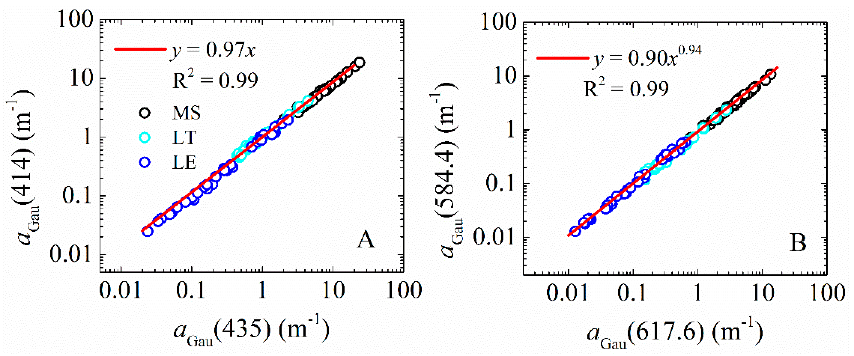
| 2 | Chl-a | 414 | 10.7 | y = 0.97x1 | 0.998 |
| 3 | Chl-a | 435 | 12 | x1 | 1 |
| 4 | Chl-c | 451.7 | 18.5 | y = 0.90x1 | 0.995 |
| 5 | Carot | 484 | 19.6 | y = 0.95x1 | 0.99 |
| 6 | Carot | 515.6 | 18 | y = 0.53x1 | 0.99 |
| 7 | PE | 548.8 | 15.7 | y = 0.76x20.92 | 0.99 |
| 8 | Chl-c | 584.4 | 17 | y = 90x20.94 | 0.997 |
| 9 | PC | 617.6 | 16 | x2 | 1 |
| 10 | Chl-c | 636 | 11.6 | y = 0.35x21.1 | 0.99 |
| 11 | Chl-b | 653 | 14 | y = 0.82x20.87 | 0.99 |
| 12 | Chl-a | 677 | 10.6 | y = 0.69x1 | 0.99 |
| 13 | others | 693.5 | 20 | y = 0.37x20.92 | 0.99 |
| Unknowns (N) | Datasets | UAPD (%) | |||
|---|---|---|---|---|---|
| Mea. | Med. | Max. | Min. | ||
| 13 | All | 47 | 43 | 73 | 24 |
| 5 | All | 37 | 38 | 46 | 27 |
| 3 | All | 33 | 34 | 40 | 25 |
| 2 | All | 32 | 34 | 38 | 24 |
| 13 | MS | 38 | 41 | 81 | 13 |
| 5 | MS | 29 | 28 | 50 | 15 |
| 3 | MS | 25 | 29 | 35 | 15 |
| 2 | MS | 26 | 28 | 37 | 16 |
| 13 | LT | 42 | 36 | 71 | 23 |
| 5 | LT | 37 | 38 | 47 | 25 |
| 3 | LT | 35 | 34 | 47 | 24 |
| 2 | LT | 32 | 31 | 49 | 22 |
| 13 | LE | 64 | 60 | 111 | 39 |
| 5 | LE | 45 | 45 | 56 | 36 |
| 3 | LE | 41 | 40 | 49 | 33 |
| 2 | LE | 39 | 39 | 50 | 33 |
| 13 | LE-2014 | 62 | 65 | 108 | 30 |
| 5 | LE-2014 | 31 | 28 | 45 | 17 |
| 3 | LE-2014 | 27 | 28 | 35 | 16 |
| 2 | LE-2014 | 22 | 21 | 33 | 16 |
| Index | All-Band | OLCI | MERIS | MODIS | VIIRS | MSI | OLI |
|---|---|---|---|---|---|---|---|
| 1 | 400 | 400 | |||||
| 2 | 412 | 413 | 413 | 412 | 410 | ||
| 3 | 443 | 443 | 443 | 443 | 443 | 444 | 443 |
| 4 | 490 | 490 | 490 | 488 | 486 | 497 | 483 |
| 5 | 510 | 510 | 510 | ||||
| 6 | 530 | 531 | |||||
| 7 | 555 | 560 | 560 | 547 | 551 | 560 | 563 |
| 8 | 620 | 620 | 620 | ||||
| 9 | 645 | 645 | |||||
| 10 | 655 | 655 | |||||
| 11 | 665 | 665 | 665 | 667 | 665 | ||
| 12 | 675 | 674 | 678 | 671 | |||
| 13 | 681 | 681 | 681 | ||||
| 14 | 709 | 709 | 709 | 704 | |||
| 15 | 745 | 754 | 754 | 748 | 745 | 740 |
| Bands | UAPD (%) | |||
|---|---|---|---|---|
| Mea. | Med. | Max. | Min. | |
| ALL-band | 30 | 32 | 36 | 23 |
| OLCI | 35 | 36 | 41 | 28 |
| MERIS + 754 | 32 | 33 | 39 | 27 |
| MERIS | 35 | 36 | 41 | 28 |
| MODIS | 34 | 33 | 40 | 30 |
| MODIS-645 | 34 | 33 | 43 | 29 |
| MODIS-748 | 45 | 45 | 50 | 40 |
| VIIRS | 36 | 34 | 48 | 31 |
| MSI | 35 | 34 | 45 | 32 |
| OLI | 48 | 46 | 63 | 42 |
| UAPD (%) | P1 | P2 | P3 | P4 | P5 | P6 | P7 | P8 | P9 | P10 | P11 | P12 | P13 |
|---|---|---|---|---|---|---|---|---|---|---|---|---|---|
| ALL-band | 29 | 23 | 23 | 19 | 20 | 20 | 14 | 22 | 19 | 18 | 36 | 21 | 18 |
| OLCI | 29 | 23 | 23 | 19 | 19 | 21 | 17 | 21 | 21 | 22 | 36 | 24 | 22 |
| MERIS + 754 | 26 | 21 | 20 | 18 | 20 | 22 | 16 | 23 | 23 | 23 | 37 | 26 | 21 |
| MERIS | 27 | 21 | 22 | 17 | 19 | 21 | 17 | 23 | 23 | 24 | 37 | 25 | 22 |
| MODIS | 33 | 27 | 28 | 23 | 21 | 22 | 17 | 22 | 21 | 18 | 35 | 24 | 29 |
| MODIS-645 | 32 | 26 | 24 | 24 | 19 | 22 | 17 | 18 | 17 | 17 | 31 | 24 | 27 |
| MODIS-748 | 45 | 39 | 40 | 35 | 31 | 30 | 27 | 29 | 25 | 28 | 32 | 29 | 40 |
| VIIRS | 33 | 29 | 28 | 25 | 25 | 25 | 24 | 29 | 26 | 24 | 40 | 27 | 28 |
| MSI | 30 | 26 | 27 | 21 | 27 | 27 | 25 | 31 | 29 | 28 | 46 | 33 | 25 |
| OLI | 31 | 30 | 32 | 27 | 33 | 30 | 26 | 33 | 35 | 41 | 46 | 43 | 29 |
| Peaks | aGau(λ) | HICO | MODIS | ||
|---|---|---|---|---|---|
| Mea. | Med. | Mea. | Med. | ||
| 1 | 386.6 | 27 | 26 | 28 | 27 |
| 2 | 414 | 21 | 20 | 23 | 19 |
| 3 | 435 | 19 | 18 | 20 | 16 |
| 4 | 451.7 | 17 | 15 | 18 | 15 |
| 5 | 484 | 18 | 16 | 17 | 13 |
| 6 | 515.6 | 19 | 14 | 19 | 14 |
| 7 | 548.8 | 24 | 23 | 33 | 32 |
| 8 | 584.4 | 29 | 26 | 44 | 45 |
| 9 | 617.6 | 34 | 28 | 45 | 37 |
| 10 | 636 | 37 | 39 | 48 | 53 |
| 11 | 653 | 32 | 25 | 34 | 29 |
| 12 | 677 | 24 | 25 | 26 | 27 |
| 13 | 693.5 | 54 | 48 | 78 | 75 |
© 2017 by the authors. Licensee MDPI, Basel, Switzerland. This article is an open access article distributed under the terms and conditions of the Creative Commons Attribution (CC BY) license (http://creativecommons.org/licenses/by/4.0/).
Share and Cite
Wang, G.; Lee, Z.; Mouw, C. Multi-Spectral Remote Sensing of Phytoplankton Pigment Absorption Properties in Cyanobacteria Bloom Waters: A Regional Example in the Western Basin of Lake Erie. Remote Sens. 2017, 9, 1309. https://doi.org/10.3390/rs9121309
Wang G, Lee Z, Mouw C. Multi-Spectral Remote Sensing of Phytoplankton Pigment Absorption Properties in Cyanobacteria Bloom Waters: A Regional Example in the Western Basin of Lake Erie. Remote Sensing. 2017; 9(12):1309. https://doi.org/10.3390/rs9121309
Chicago/Turabian StyleWang, Guoqing, Zhongping Lee, and Colleen Mouw. 2017. "Multi-Spectral Remote Sensing of Phytoplankton Pigment Absorption Properties in Cyanobacteria Bloom Waters: A Regional Example in the Western Basin of Lake Erie" Remote Sensing 9, no. 12: 1309. https://doi.org/10.3390/rs9121309