
Modeling the Spatiotemporal Dynamics of Gross Domestic Product in China Using Extended Temporal Coverage Nighttime Light Data


1
Chongqing Key Laboratory of Karst Environment, School of Geographical Sciences, Southwest University, Beibei, Chongqing 400715, China
2
Norwegian Institute of Bioeconomy Research (NIBIO), 1431 Ås, Norway
3
CEES, Department of Biosciences, University of Oslo, Blindern, 0316 Oslo, Norway
*
Author to whom correspondence should be addressed.
Remote Sens. 2017, 9(6), 626; https://doi.org/10.3390/rs9060626
Submission received: 12 May 2017
/
Revised: 12 June 2017
/
Accepted: 15 June 2017
/
Published: 18 June 2017
(This article belongs to the Special Issue Recent Advances in Remote Sensing with Nighttime Lights)
Abstract
:Nighttime light data derived from the Defense Meteorological Satellite Program’s Operational Linescan System (DMSP-OLS) in conjunction with the Soumi National Polar-Orbiting Partnership Visible Infrared Imaging Radiometer Suite (NPP-VIIRS) possess great potential for measuring the dynamics of Gross Domestic Product (GDP) at large scales. The temporal coverage of the DMSP-OLS data spans between 1992 and 2013, while the NPP-VIIRS data are available from 2012. Integrating the two datasets to produce a time series of continuous and consistently monitored data since the 1990s is of great significance for the understanding of the dynamics of long-term economic development. In addition, since economic developmental patterns vary with physical environment and geographical location, the quantitative relationship between nighttime lights and GDP should be designed for individual regions. Through a case study in China, this study made an attempt to integrate the DMSP-OLS and NPP-VIIRS datasets, as well as to identify an optimal model for long-term spatiotemporal GDP dynamics in different regions of China. Based on constructed regression relationships between total nighttime lights (TNL) data from the DMSP-OLS and NPP-VIIRS data in provincial units (R2 = 0.9648, P < 0.001), the temporal coverage of nighttime light data was extended from 1992 to the present day. Furthermore, three models (the linear model, quadratic polynomial model and power function model) were applied to model the spatiotemporal dynamics of GDP in China from 1992 to 2015 at both the country level and provincial level using the extended temporal coverage data. Our results show that the linear model is optimal at the country level with a mean absolute relative error (MARE) of 11.96%. The power function model is optimal in 22 of the 31 provinces and the quadratic polynomial model is optimal in 7 provinces, whereas the linear model is optimal only in two provinces. Thus, our approach demonstrates the potential to accurately and timely model long-term spatiotemporal GDP dynamics using an integration of DMSP-OLS and NPP-VIIRS data.

1. Introduction
Gross Domestic Product (GDP) is one of the most important parameters for the analysis of national or regional economic development [1]. However, GDP is often inadequately measured in developing countries due to the poor governmental statistical infrastructure [2,3]. Worse, economic statistical data may be manipulated by local governments to meet the targets [4]. Furthermore, the release of economic statistic data is lagging behind [4,5]. For example, statistical data of current year in the China Statistical Yearbook are usually published in the next year from September to October [6]. This increases the difficulties to obtain accurate and up-to-date GDP data in developing countries. Therefore, more appropriate measures are needed to supplement the statistical data for the estimating and mapping of the GDP in a statistical area [7].
The nighttime light data obtained by the Operational Linescan System (OLS) flown by the U.S. Air Force Defense Meteorological Satellite Program (DMSP) are an effective proxy for socioeconomic activity. DMSP-OLS data provide a powerful remote sensing tool to model the spatiotemporal dynamics of GDP at a large spatial scale [8]. For example, Elvidge et al. [9] first discovered a strong correlation (R2 = 0.97) between nighttime light area and GDP in 21 countries in the Americas during the mid-1990s, then the relationship was confirmed for a larger number of countries [10,11]. Ebener et al. [12] estimated the GDP per capita for 171 countries at the country level and 26 countries from 5 continents at the sub-national level. Howerer, the results showed a significant over estimation for 10 countries and an under estimation for most of the high income countries. Based on the work of Ebener et al. [12], Sutton et al. improved the method by aggregating the urban population [13]. Then the method was applied to estimate the GDP for 4 countries (China, India, Turkey and the United States) at the sub-national level, and the results indicated that the method was superior to which proposed by Ebener et al. in many cases. There are also many studies focused on the global scale. For example, Doll et al. [10] first created a global GDP map by considering the relationship between nighttime light area and socioeconomic parameters at the country level. That study estimated the total GDP of the world to be 22.1 trillion dollars, which was about 80% of the World Resource Institute’s statistics for 1992. Combining nighttime lights, population density and land cover data, Ghosh et al. [2] created a global GDP map with a 1 km spatial resolution. Then the map was validated by comparing the estimated GDP with the official GDP, and the results showed that the estimated GDP was greater than official GDP for almost all administrative units. This product has been released by the National Oceanic and Atmospheric Administration’s National Geophysical Data Center (NOAA/NGDC) [14]. Elvidge et al. [15] analyzed the relationships among nighttime light data, population, GDP and improvements in lighting efficiency on a global scale from 1992 to 2012 and defined national lighting trends across seven categories. Wu et al. [4] analyzed numerous factors affecting the relationship between nighttime lights and GDP on a global scale and concluded that agriculture is responsible for approximately 25.4% of total light consumption. In recent years, studies have been further conducted to model GDP using nighttime light data in China. Zhao et al. [16] first mapped the spatiotemporal dynamics of the GDP between 1996 and 2000 in China using DMSP-OLS data. The results showed that the error rates between the estimated and actual GDP were relatively small for the 12 provinces with the largest GDP while the relatively large errors were generated in some small GDP provinces. Thereafter, Ma et al. [17] discovered a quantitative relationship between long-term nighttime light data and GDP for individual cities in China, and concluded that temporal changes in nighttime light brightness could be statistically significantly associated with GDP dynamics in most individual cities.
With a temporal coverage ranging from 1992 to 2013, the DMSP-OLS dataset provides the longest continuous time series of global urban remote sensing products [15]. However, the DMSP-OLS ceased operation in 2013, following which there are no data. On October 28, 2011, the National Aeronautics and Space Administration (NASA) and NOAA launched the Soumi National Polar-Orbiting Partnership (NPP), which carries the Visible Infrared Imaging Radiometer Suite (VIIRS), to collect low light imaging data [18]. In early 2013, nighttime light composite data were released by the NOAA/NGDC [19]. As a new generation of nighttime light data, the NPP-VIIRS data demonstrate several improvements over the DMSP-OLS data [20]. For example, the spatial resolution of the NPP-VIIRS data (15 arc-seconds) is higher than that of the DMSP-OLS data (30 arc-seconds). In addition, the NPP-VIIRS data are not characterized by the saturation of bright lights that exists within the DMSP-OLS data [20]. Moreover, the NPP-VIIRS system employs on-board calibration, which was lacking with the DMSP-OLS [21]. Compared with DMSP-OLS, therefore, NPP-VIIRS provides a more powerful approach to research the nighttime light.
The People’s Republic of China has been experiencing rapid economic growth at an unprecedented speed since the reform and opening up policy in the late 1970s, being the second largest economy in the world in 2010 [22,23,24]. Several studies have been carried out to generate a comparison between GDP modeling using DMSP-OLS data and modeling using NPP-VIIRS data [5,25,26]. However, few methods have been proposed to integrate the DMSP-OLS and NPP-VIIRS data to construct a consistent model, which is of great importance to understand the long-term economic development in China. Furthermore, most of the previous studies have attempted to model GDP with nighttime light data using a single function model at all spatial levels [5,13,15,16,25] or using different function models at different spatial levels [17,26]. With an area of 9.6 million square kilometers, China has substantial regional variation with regard to natural environments and socioeconomic development patterns [27], so the quantitative relationship between nighttime lights and GDP also varies across different regions of China [15,24]. Thus, different function models should be applied based on individual economic development patterns in order to obtain more accurate modeling results [15,24].
To fill the research gap, the current study contains two major objectives. The first is to develop a simple method for integrating DMSP-OLS and NPP-VIIRS data to extend the temporal coverage of nighttime light data. The second objective is to identify the optimal models with which to model the spatiotemporal dynamics of GDP in China’s different regions using nighttime light data.
2. Materials
The Version 4 DMSP-OLS nighttime light time series dataset from 1992 to 2013 was obtained from the NOAA’s National Centers for Environmental Information (NCEI, formerly NGDC) website [28]. There are three types of annually averaged data in the dataset: cloud free coverage, average visible and stable lights. Among the three types of data, stable light data contain lights derived from cities, towns and other sites with persistent lighting, while fires, volcanoes, background noise and other ephemeral events have been discarded [29]. The DMSP-OLS nighttime stable light (NSL) data have a spatial resolution of 30 arc-seconds, a coverage spanning −180 to 180 degrees longitude and −65 to 75 degrees latitude. The digital number (DN) value for pixels ranges from 0 to 63. This means that value 0 represents the unlit area and the greater the value, the higher the light level of the region will be. In addition, the NOAA/NCEI website has released a global radiance calibrated nighttime light (RCNL) dataset without sensor saturation, which can be used as the ideal reference data for the intercalibration of the DMSP-OLS NSL dataset [30,31,32,33,34].
The NPP-VIIRS nighttime light data from 2012 to 2015 were also obtained from the NOAA/NCEI website [35]. These data comprise monthly averaged radiance composite data that span from April 2012 to December 2015. Because the monthly averaged data possess a high quality with a reliable temporal consistency [36], we selected NPP-VIIRS monthly averaged data from December 2012 to December 2015 for this study. The NPP-VIIRS data have a spatial resolution of 15 arc-seconds and lack saturation problems [20]. However, as it is a preliminary product, the NPP-VIIRS data have not been filtered to remove light detections associated with gas flares, fires, volcanoes or aurorae, and the dataset has not been processed to remove background noise.
The administrative boundary data of China, including all of the national and provincial boundaries, were obtained from the National Geomatics Center of China. All of the nighttime light data were extracted according to Chinese administrative boundaries and were then resampled to one square kilometer grids within a Lambert Azimuthal Equal Area projection to facilitate calculation.
The GDP statistical data from 1992 to 2015 for both national and provincial level units were derived from the China Statistical Yearbook. Taiwan, Hong Kong and Macao are excluded in this study because of the lack of GDP statistical data. The Chinese currency unit used for the GDP is Renminbi (RMB), also known as Yuan in Chinese.
3. Methods
Four major steps are employed herein to model the spatiotemporal dynamics of GDP using the extended temporal coverage nighttime light dataset: first, correcting the DMSP-OLS data from 1992 to 2013; second, correcting the NPP-VIIRS data from 2012 to 2015; third, extending the temporal coverage of nighttime data with the DMSP-OLS data and NPP-VIIRS data; and fourth, modeling the spatiotemporal dynamics of GDP in China from 1992 to 2015.
3.1. Correction of the DMSP-OLS Data
As mentioned above, there are several shortcomings with the DMSP-OLS data [20]. These shortcomings limit the potential reliability and accuracy for modeling the long-term dynamics of GDP or other socioeconomic parameters [5,37]. Therefore, it is necessary to correct the DMSP-OLS data to improve the data continuity and accuracy [38].
3.1.1. Intercalibration
To correct for the discontinuity and inaccuracy that may result from modeling the GDP using the DMSP-OLS data, resulting from a lack of on-board calibration and a saturation of bright lights, we intercalibrated the DMSP-OLS data from 1992 to 2013 following the invariant region method proposed by previous studies [33,34,38,39,40,41]. Japan was selected as the invariant region [41], and the 2006 RCNL data were selected as the reference data [33]. Then, the DMSP-OLS data from 1992 to 2013 were intercalibrated using the following regression model [34]:
where DN is the original DN value of the DMSP-OLS data, DNcalibrated is the DN value after intercalibration, and a and b are coefficients. These coefficients are shown in Table 1 [34].
3.1.2. Intra-Annual Composition
In certain years, the DMSP-OLS data were collected from two satellites simultaneously. To make full use of the information derived from multiple satellites, we obtained the intra-annual composite DMSP-OLS data using Equation (2) [38]:
where DNa(n,i) and DNb(n,i) are the DN values of the ith lit pixel from two DMSP-OLS datasets in the nth year after intercalibration, and DN(n,i) is the DN value of the ith lit pixel in the nth year after intra-annual composition.
3.1.3. Inter-Annual Series Correction
Since most regions in China have been experiencing continuous GDP growth over the past nearly four decades, we assumed that the DN value of each pixel detected in a given year should not be smaller than the DN value detected for the same pixel in the previous year [38]. Accordingly, we corrected the DMSP-OLS data from 1992 to 2013 using Equation (3) [38]:
where DN(n−1,i), DN(n,i) and DN(n+1,i) are the DN values of the ith lit pixel of the DMSP-OLS data in the (n − 1)th, nth and (n + 1)th years, respectively.
To avoid DN values within the DMSP-OLS data reduced largely in the first few years, we also corrected the DMSP-OLS data from 1992 to 2013 using Equation (4) to ensure that the DN value of each pixel detected in an earlier year is not larger than the DN value detected in a later year [39]:
where DN(n−1,i), DN(n,i) and DN(n+1,i) represent the DN values of the ith lit pixel of the DMSP-OLS data in the (n − 1)th, nth and (n + 1)th years, respectively. In this way, we obtained DMSP-OLS data from 1992 to 2013 with inter-annual series correction by averaging the corrected results using Equations (3) and (4).
3.2. Correction of the NPP-VIIRS Data
As a preliminary dataset, NPP-VIIRS data have not been filtered to remove light detections associated with gas flares, fires, volcanoes, aurorae and background noise. These noises may limit the reliability and accuracy of the data for GDP modeling. Therefore, we employed the method proposed by Shi et al. [5] to reduce these negative factors. This method contains three major steps: (a) Considering that very few DN values of lit pixels should increase from zero to positive [25], we assumed that the lit areas within the NPP-VIIRS data from 2012 to 2015 and those within the 2012 DMSP-OLS data were equivalent. Thus, a mask was created by extracting the 2012 DMSP-OLS data whose DN values were positive, and the primary correction NPP-VIIRS data from 2012 to 2015 were generated by extracting values utilizing the mask. (b) Since Beijing, Shanghai and Guangzhou are the three most developed cities in China, the DN values of lit pixels in other areas should not exceed those of the three megacities, in theory. Optimal threshold values for the NPP-VIIRS data from 2012 to 2015 were assigned based on this hypothesis, after which the DN value of each lit pixel that exceeded the designated threshold was assigned the maximum DN value within the pixel’s immediate eight neighbors. (c) Finally, the DN values of lit pixels less than zero were assigned a zero value.
3.3. Temporal Coverage Extension of the Nighttime Light Data
The temporal coverage of the DMSP-OLS data spans the period of 1992–2013, and the acquisition of VIIRS data is ongoing [42]. The different settings of the sensors used to acquire the DMSP-OLS and NPP-VIIRS data may cause difficulties in integrating these two datasets for the continuous modeling of the spatiotemporal dynamics of GDP in China since the 1990s. Consequently, a simple method was developed in this study to extend the temporal coverage of nighttime light data.
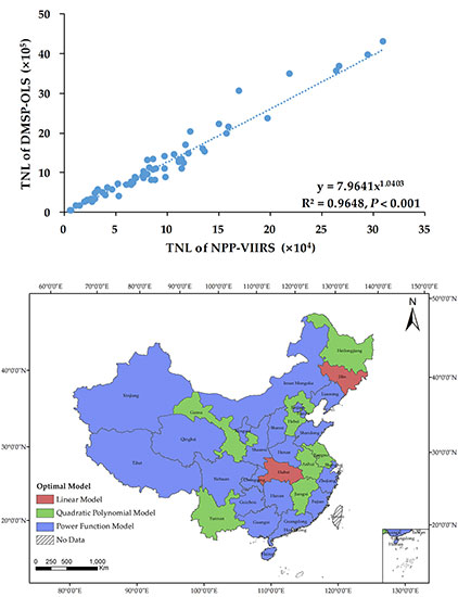
Total nighttime lights (TNL) is defined as the cumulative DN value of all lit pixels within a corresponding administrative region [43]. Most of the previous studies that modeled the dynamics of the GDP or other socioeconomic parameters using nighttime light data were based on the construction of statistical relationships between TNL and a particular socioeconomic parameter [13,26,37,40,43,44,45]. By examining the scattergram composed of TNL from the DMSP-OLS and NPP-VIIRS data at the provincial level of China from 2012 to 2013, which is the overlap period when the nighttime light data were collected by both sensors, we were able to observe sharply defined diagonal clusters of points (Figure 1a).
For further analysis, we developed a linear regression model, a quadratic polynomial regression model and a power function regression model relating TNL from the DMSP-OLS and NPP-VIIRS data in provincial units from 2012 to 2013 (Figure 1b–d). The results suggest the existence of a strong correlation between the TNL from the DMSP-OLS and NPP-VIIRS data at the provincial level. Moreover, among the three regression models, the power function model has the highest coefficient of determination (R2 = 0.9648, P < 0.001) (Figure 1d).
Based on the results of the regression analyses above, a method was proposed to generate the TNL for the extended temporal coverage nighttime light data using Equation (5):
where TNLan and TNLbn are the TNL for the DMSP-OLS data and NPP-VIIRS data in the corresponding administrative region in the nth year, respectively, and TNLn is the TNL for the extended temporal coverage nighttime light data in the nth year.
3.4. Modeling the Spatiotemporal Dynamics of the GDP
A few models have been applied to model the GDP or other socioeconomic parameters using nighttime light data [5,17,46,47]. Since economic development patterns vary with natural environment and geographical location [27], we applied three simple regression models, namely, the linear model (Equation (6)), quadratic polynomial model (Equation (7)) and power function model (Equation (8)), to uncover the optimal GDP dynamics models using nighttime data among China’s different regions over time:
where GDPestimated is the estimated GDP of an administrative region in a particular year, TNL is the TNL for the extended temporal coverage data in the corresponding administrative region in the same year, and a, b and c are coefficients.
The coefficient of determination, which is usually denoted as R2, is the primary indicator to evaluate the performance of a model relating observed and estimated values [48]. We also employed the mean absolute relative error (MARE) to assess the overall accuracy of the models [49]:
where n is the number of years or administrative regions, and REi is the ith relative error (RE) of the corresponding year or administrative region, which can be calculated using Equation (10):
where GDPestimated is the estimated GDP, and GDPstatistical is the statistically computed GDP.
4. Results
4.1. Extended Temporal Coverage Results for the Nighttime Light Data
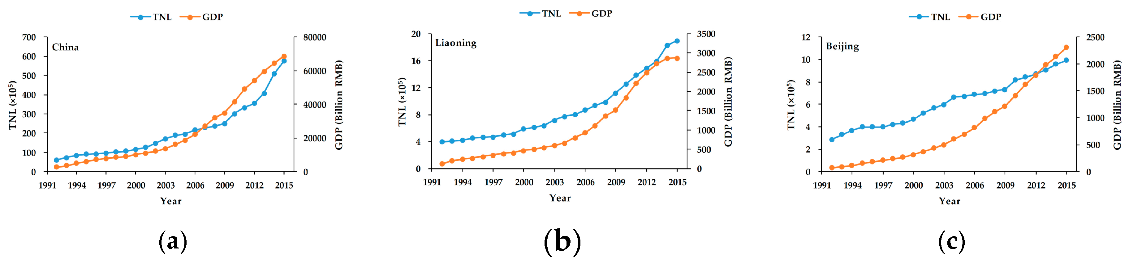
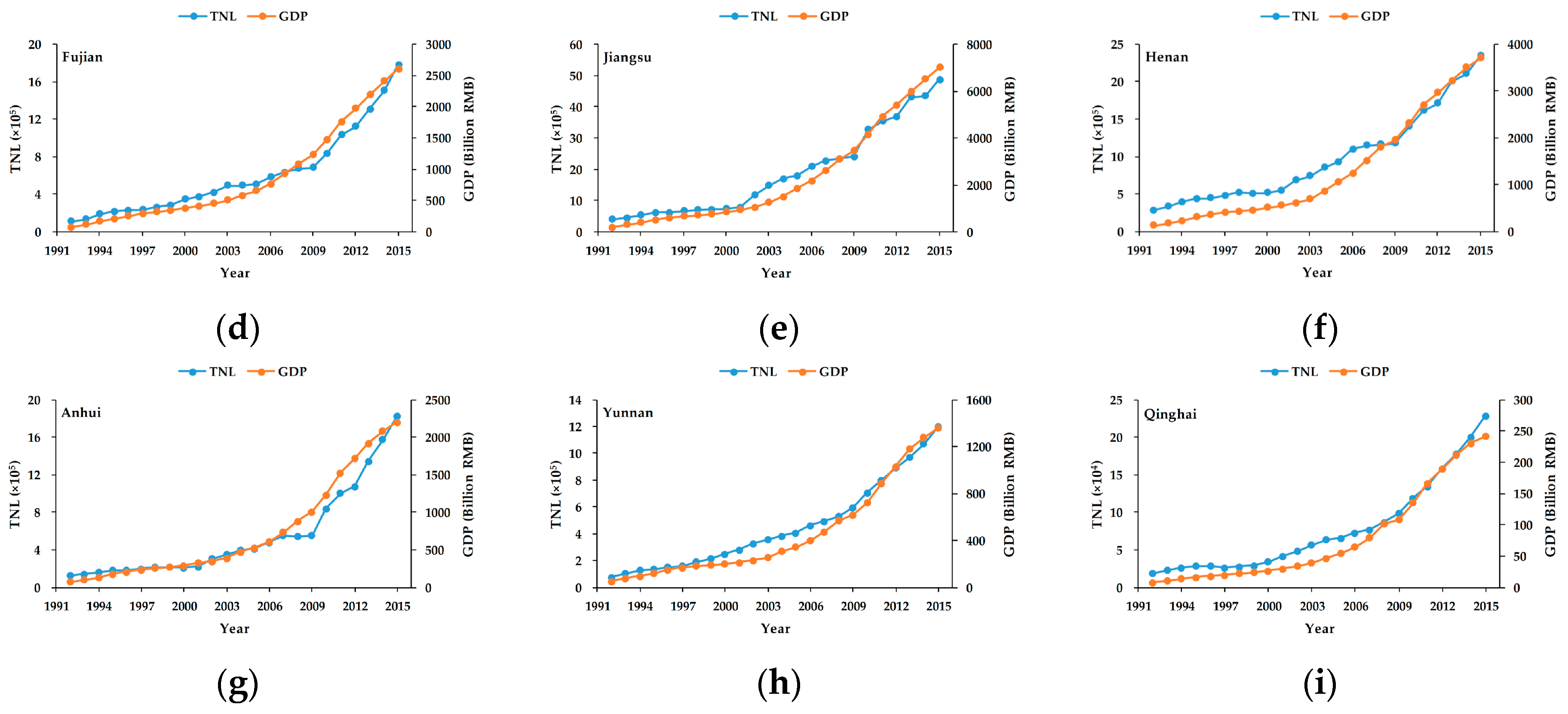
Figure 2 illustrates the extended temporal coverage results for nighttime light data at the country (Figure 2a) and provincial (Figure 2b–i) levels. For the provincial level analysis, eight provinces (Liaoning, Beijing, Fujian, Jiangsu, Henan, Anhui, Yunnan and Qinghai) were selected as instances according to the eight economic regions subdivided by the Coordinated Regional Development Strategy and Policy Reports published by the Development Research Center of the State Council of China [50]. The results indicate that the TNL derived from the extended temporal coverage data have a high degree of continuity in the time series from 1992 to 2015 at both the country and provincial levels (Figure 2). Additionally, the GDP of each of the regions from 1992 to 2015 were also compared with the TNL, which confirms that the trends in the TNL and the trends in the GDP are highly consistent (Figure 2), as indicated by previous studies [2,13,16].
In 2012 and 2013, the nighttime light data were acquired by the OLS and VIIRS sensors simultaneously. Although the TNL values from the extended temporal coverage data were generated from 2014, we are capable of assessing the accuracy of the extended temporal coverage data through a comparison between the TNL generated using NPP-VIIRS data and the TNL generated using DMSP-OLS data for 2012 and 2013 (Table 2). As shown in Table 2, the MARE values of the TNL generated from the extended temporal coverage data are 13.83% and 12.97% in 2012 and 2013, respectively, while the RE values of the TNL vary in different provinces and years. For example, in 2012, the maximum and minimum absolute RE values are 36.1% and 0.05% for Shanghai and Beijing, respectively. Meanwhile, in 2013, the maximum and minimum absolute RE values are 59.16% and 0.69% for Guizhou and Gansu, respectively.
To further assess the accuracy of the TNL derived from the extended temporal coverage data, we classified the absolute RE values into three categories: 0–25% as highly accurate, 25–50% as moderately accurate and >50% as inaccurate [5,25]. We subsequently calculated the percent of provinces within each category for all of the 31 provinces for each year (Table 3). The TNL derived from the extended temporal coverage data exhibit a high quality at the provincial level and are characterized by highly accurate percentages of 83.87% and 90.32% in 2012 and 2013, respectively. Moreover, the corresponding inaccurate percentages are 0% and 3.23% in 2012 and 2013, respectively. Therefore, these results indicate that the method proposed above is reliable for the temporal coverage extension of nighttime light data among the provincial regions in China.
4.2. Modeling Results for the Spatiotemporal Dynamics of the GDP
Using the extended temporal coverage nighttime light data, we modeled the spatiotemporal dynamics of the GDP from 1992 to 2015 at both the country and provincial levels. Three regression models were applied: a linear model, a quadratic polynomial model and a power function model. Note that all of the models developed herein are significant (P < 0.001).
4.2.1. Modeling Results at the Country Level
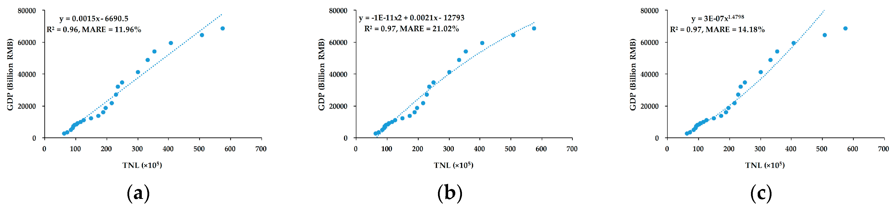
Through the three regression models mentioned above, the long-term relationship between the TNL and GDP in China from 1992 to 2015 was analyzed (Figure 3). The R2 values obtained from three models are 0.96, 0.97 and 0.97, respectively, which all represent high correlations and have no marked difference. However, the MARE values vary among the different regression models. For example, the maximum MARE value is 21.02% in the quadratic polynomial model, whereas the minimum MARE value is 11.96% in the linear model. This indicates that some details in the relationship between the TNL and GDP may be ignored when the optimal model is selected solely based on the R2 values. Thus, these results indicate that all of the three regression models can appropriately reflect the long-term GDP dynamics in China using the extended temporal coverage data and that the linear model is optimal at the country level, with the lowest MARE value.
Referring to the approach proposed by He et al. [37], the accuracy of GDP modeling in time series using the extended temporal data was assessed further through a comparison with the GDP modeling using DMSP-OLS data (1992–2013) and NPP-VIIRS data (2014–2015) in provincial units for each year (Figure 4). The results for this process are exhibited in Table 4. All of the regression analyses were performed using a linear model. As shown in Table 4, the MARE of the model utilizing the extended temporal data is 11.96%, whereas that of the model using DMSP-OLS data and NPP-VIIRS data is 18.94%. Moreover, all of the absolute RE values of the models employing the extended temporal data are less than or equal to 35.61%. Therefore, modeling the long-term dynamics of GDP in China from 1992 to 2015 using the extended temporal data is reliable compared to the previous results [15,17,33,38].
4.2.2. Modeling Results at the Provincial Level
The long-term relationship between the TNL and GDP at the provincial level from 1992 to 2015 was analyzed using the three regression models, and the R2 and MARE values for each of the three models for each province were calculated accordingly (Table 5). As shown in Table 5, the mean R2 values of the linear models, quadratic polynomial models and power function models are 0.95, 0.97 and 0.96, respectively, while the mean MARE values vary more markedly. Furthermore, the R2 values of the three models are very similar among most of the provinces, whereas the MARE values vary substantially with the different models for each province. It can be concluded that at the provincial level, all of the three models are reliable for modeling the long-term GDP dynamics using the extended temporal coverage data. In general, the power function model is the best-fitting model, with the minimum mean MARE value of 14.91%, which is supported by previous studies [17,26].
To further ascertain the most effective provincial-level models, the optimal models for each province were chosen through a comparison of the R2 and MARE values of each model (Figure 5). The power function model is found to be optimal for modeling the dynamics of the GDP from 1992 to 2015 using the extended temporal coverage data for most of the provinces (22 of the 31 provinces), while the quadratic polynomial model is optimal in seven provinces (Heilongjiang, Hebei, Gansu, Jiangsu, Anhui, Jiangxi and Yunnan). The linear model is only the best-fitting model for two provinces, Jilin and Hubei. Consequently, although the power function model is generally the best-fitting model for long-term modeling of GDP dynamics using the extended temporal coverage data at the provincial level, the optimal model varies for different regions of China.
Three provinces (Hubei, Gansu and Guangdong) were selected as respective test instances for each model (Figure 6). The results obtained from employing the quadratic polynomial model for the long-term modeling of GDP dynamics using the extended temporal data imply that TNL growth was relatively faster than economic growth in the corresponding province from 1992 to 2015, while the power function model implies that the economy grew more quickly than the TNL. Subsequently, the gaps in the growth rates between the TNL and GDP were further analyzed at the provincial level using the power function model, which was previously determined to be the general optimal model at the provincial level. The results of this analysis using the value of coefficient b (Equation (8)) as a scaling exponent with which to measure the gaps in the growth rates between TNL and GDP are exhibited in Figure 7.
The results illustrate that the gaps in the growth rates between the TNL and GDP exhibit an evident regional differentiation throughout China. The gaps are relatively smaller in most of the undeveloped southwestern provinces, including Tibet, Yunnan and Guizhou. In the majority of the northwestern provinces, such as Xinjiang, Qinghai and Gansu, the gaps are also relatively small. In contrast, the gaps in the growth rates between TNL and GDP are relatively larger in the central and eastern provinces of China. For example, substantially higher gaps are observed in Beijing, Tianjin, Shanghai and Guangdong, wherein the core urban areas demonstrate more intensive commerce and industry relative to other regions of China [51]. Therefore, since the quantitative relationship between nighttime lights and GDP varies across different regions of China, it is concluded that regression models for the modeling of long-term GDP dynamics using the extended temporal data should be applied specifically based on the individual socioeconomic developmental pattern in the corresponding region in order to establish more accurate modeling [17].
5. Discussion
The DMSP-OLS data, representing the most widely used nighttime light data over the previous two decades [52], possess a temporal coverage spanning 1992–2013, while NPP-VIIRS data have been available since 2012 and represent the new generation of nighttime light data. In spite of great significance to study long-term socioeconomic developmental patterns, few studies have been conducted for integrating the two datasets in order to continuously monitor the economic development, for example in China since the 1990s. This challenge primarily originates from the following reasons: first, the OLS and VIIRS sensors have different configurations; and second, specific and notable shortcomings exist within the two datasets [20].
A simple method has been proposed in this study to integrate the DMSP-OLS and NPP-VIIRS data in order to extend the temporal coverage of nighttime light data. The results demonstrate that the TNL derived from the extended temporal data exhibits good quality and a generally reliable temporal consistency. Considering that most of the previous studies employed to deduce the behavior of socioeconomic development using nighttime data were conducted by constructing statistical relationships between the TNL and socioeconomic parameters [13,26,37,40,43,44,45], the method proposed in the current study is suitable for the estimation of long-term socioeconomic parameters as well as the modeling of spatiotemporal dynamics using nighttime light data.
Using the extended temporal coverage nighttime light data, the long-term spatiotemporal dynamics of GDP in China were modeled at both the country and provincial levels. The results indicate that nighttime lights can be a useful indicator for measuring economic development, which has been proven by a number of previous studies [5,13,17,26,37,53]. The regression model employed to estimate regional socioeconomic parameters should be constructed using nighttime light data and statistical data from the same country or region [25]. Therefore, previous studies aiming to model the socioeconomic development using nighttime light data were primarily focused on constructing statistical relationships between nighttime lights and socioeconomic parameters derived from samples obtained at the same administrative level for each year [16,37,54]. Since we have obtained nighttime light data with an extended temporal coverage through the method proposed in this study, time series regression models were developed for each region at the provincial level. Compared with the models developed in previous studies [16,37,54], errors induced by the regional differences have been eliminated in the current study. Therefore, this study has provided a feasible approach for the accurate long-term modeling of dynamic socioeconomic parameters using nighttime light data.
One of the main objectives of this study is to identify the optimal models for the long-term modeling of GDP dynamics using nighttime light data at both the country and provincial levels. The results show that the linear regression model is the best-fitting model at the country level, exhibiting the lowest MARE value compared with the quadratic polynomial model and power function model. At the provincial level, the optimal model is generally the power function model, similar to the conclusions reached by previous investigations [17,26]. The implication of power function regression for the modeling of long-term GDP dynamics using nighttime light data is a temporal lag in the growth of nighttime lights compared with the relatively faster growth in the economy [17]. Considering that the official data of economic development indicated a rapid growth throughout most regions of China, the results of this study are credible [55]. Furthermore, we have chosen the optimal models for the modeling of long-term GDP dynamics using nighttime light data for each of the provinces of China. The power function model is the best-fitting model in most of the provinces (22 out of 31 provinces), while the quadratic polynomial model is the optimal model for seven provinces. Meanwhile, the linear model is optimal only in two provinces. Most previous examinations of dynamic socioeconomic parameter modeling using nighttime light data applied a single regression model for all of the administrative units at the same level or even at different levels [5,8,13,26,37]. Alternatively, our results indicate that different regression models should be designed based on the particular socioeconomic developmental patterns among different regions or at different administrative levels.
Using the power function regression model, the gaps in the growth rates between the TNL and GDP were further analyzed at the provincial level. Although the connection between the TNL and GDP is an empirical relationship that cannot be viewed as an absolute law [5], the results exhibit a regular pattern in the spatial distribution. For example, the relatively smaller gaps in the undeveloped western provinces were encouraged by the more recent development of industrialization and urbanization. The economic growth in these provinces primarily rely on the expansion of construction and a substantial increase in the input of production materials, which can also contribute to large increases in the TNL [56,57]. The larger gaps in the central and eastern provinces can be explained by the more advanced and efficient industrial structures in these regions [58,59,60]. However, the reasons for these large gaps vary among different regions of China [61]. For instance, the gap in the growth rates between the TNL and GDP is very large in Shanxi, which is one of the major coal production centers of China, wherein the energy industry contributes largely to GDP growth while the TNL value for stable lights increases relatively slowly.
As a preliminary attempt to integrate DMSP-OLS and NPP-VIIRS data for the continuous monitoring of long-term economic dynamics using nighttime light data, some limitations are inherent in this study. First, although the precision of the modeling of long-term GDP dynamics using nighttime light data has been improved by the data processing, the flaws that exist within the DMSP-OLS and NPP-VIIRS data could not be removed completely. These flaws therefore reduce the accuracy of the extended temporal coverage dataset, as well as of the modeling of long-term GDP dynamics using nighttime light data. Second, while the NPP-VIIRS data have a higher spatial and temporal resolution than the DMSP-OLS data, these advantages have not been integrated into the extended dataset during the synthesis of the DMSP-OLS and NPP-VIIRS data. Third, considering that three simple regression models (the linear model, quadratic polynomial model and power function model) have been applied in this study to identify the optimal model for the modeling of long-term GDP dynamics using nighttime light data, additionally complex models need to be developed in order to achieve more accurate models of regional socioeconomic activity. Therefore, with upcoming version updates for the NPP-VIIRS data and with more easy-access sources of nighttime light data, new approaches can be developed for the modeling of socioeconomic dynamics using multi-sensor nighttime light data in future studies.
6. Conclusions
Nighttime light data provide substantial potential for the modeling of the spatiotemporal dynamics of Gross Domestic Product (GDP) and other socioeconomic parameters over large areas. Traditionally, two types of nighttime light data have been employed in previous studies to address this issue. The first is nighttime light data collected by the Operational Linescan System (OLS) flown by the U.S. Air Force Defense Meteorological Satellite Program (DMSP), and the second is the data acquired by the Visible Infrared Imaging Radiometer Suite (VIIRS) carried by the Soumi National Polar-Orbiting Partnership (NPP). The DMSP-OLS data have a broad temporal coverage spanning the period of 1992–2013, while the NPP-VIIRS data are available since 2012. Unfortunately, because of an inconsistent configuration between the two sensors, few studies have been carried out to integrate the DMSP-OLS and NPP-VIIRS data to consistently monitor socioeconomic dynamics since the 1990s.
In this study, we made an attempt to integrate the DMSP-OLS data and NPP-VIIRS data to construct an extended temporal coverage dataset from 1992 to the present day. Furthermore, using the extended temporal coverage nighttime light data, three simple regression models (the linear model, quadratic polynomial model and power function model) were applied to model the spatiotemporal dynamics of GDP during the research period in China at the country and provincial levels. Our results demonstrate that at the country level, the linear model is optimal with a minimum mean absolute relative error (MARE) of 11.96%, while those of the quadratic polynomial model and power function model are 21.02% and 14.18%, respectively. At the provincial level, the best-fitting model is generally the power function model, which exhibits a mean MARE value of 14.91%. Through an additional analysis at the provincial level, it is revealed that the power function model is optimal in 22 out of the 31 provinces, while the quadratic polynomial model is the best-fitting model in 7 provinces, and the linear model is optimal only in two provinces. In conclusion, the results indicate that the current research provided a new approach with which to accurately model the long-term spatiotemporal dynamics of GDP using a combination of DMSP-OLS data and NPP-VIIRS data, which is of great importance in the analysis of regional socioeconomic development patterns since the 1990s.
Finally, since the National Centers for Environmental Information of the National Oceanic and Atmospheric Administration (NOAA/NCEI) is working to provide NPP-VIIRS nighttime light data of higher quality, future studies can be conducted in order to obtain a more comprehensive integration of the DMSP-OLS and NPP-VIIRS data.
Acknowledgments
This study was supported by the National Key Technology R&D Program of China (grant number: 2016YFC0500106), Special Project of Science and Technology Basic Work (grant number: 2014FY210800-5) and the Fundamental Research Funds for the Central Universities (grant number: XDJK2015B021 and SWU114108).
Author Contributions
Mingguo Ma and Xiaobo Zhu designed the study. Xiaobo Zhu and Wei Ge processed the data. Xiaobo Zhu, Mingguo Ma and Hong Yang drated the paper. All of the authors contributed to the result discussion and paper writing.
Conflicts of Interest
The authors declare no conflict of interest.
References
- Henderson, J.V.; Storeygard, A.; Weil, D.N. Measuring economic growth from outer space. Am. Econ. Rev. 2012, 102, 994–1028. [Google Scholar] [CrossRef] [PubMed]
- Ghosh, T.; Powell, R.L.; Elvidge, C.D.; Baugh, K.E.; Sutton, P.C.; Anderson, S. Shedding light on the global distribution of economic activity. Open Geogr. J. 2010, 3, 148–161. [Google Scholar]
- Feige, E.L.; Urban, I. Measuring underground (unobserved, non-observed, unrecorded) economies in transition countries: Can we trust GDP ? J. Compar. Econ. 2008, 36, 287–306. [Google Scholar] [CrossRef]
- Wu, J.; Wang, Z.; Li, W.; Peng, J. Exploring factors affecting the relationship between light consumption and GDP based on DMSP/OLS nighttime satellite imagery. Remote Sens. Environ. 2013, 134, 111–119. [Google Scholar] [CrossRef]
- Shi, K.; Yu, B.; Huang, Y.; Hu, Y.; Yin, B.; Chen, Z.; Chen, L.; Wu, J. Evaluating the ability of NPP-VIIRS nighttime light data to estimate the gross domestic product and the electric power consumption of China at multiple scales: A comparison with DMSP-OLS data. Remote Sens. 2014, 6, 1705–1724. [Google Scholar] [CrossRef]
- National Bureau of Statistics of the People’s Republic of China. Available online: http://www.stats.gov.cn/tjzs/cjwtjd/201407/t20140714_580886.html (accessed on 11 November 2016).
- Henderson, V.; Storeygard, A.; Weil, D.N. A bright idea for measuring economic growth. Am. Econ. Rev. 2011, 101, 194–199. [Google Scholar] [CrossRef] [PubMed]
- Chen, X.; Nordhaus, W.D. Using luminosity data as a proxy for economic statistics. Proc. Natl. Acad. Sci. USA 2011, 108, 8589–8594. [Google Scholar] [CrossRef] [PubMed]
- Elvidge, C.D.; Baugh, K.E.; Kihn, E.A.; Kroehl, H.W.; Davis, E.R.; Davis, C.W. Relation between satellite observed visible-near infrared emissions, population, economic activity and electric power consumption. Int. J. Remote Sens. 1997, 18, 1373–1379. [Google Scholar] [CrossRef]
- Doll, C.H.; Muller, J.-P.; Elvidge, C.D. Night-time imagery as a tool for global mapping of socioeconomic parameters and greenhouse gas emissions. Ambio 2000, 29, 157–162. [Google Scholar] [CrossRef]
- Elvidge, C.D.; Imhoff, M.L.; Baugh, K.E.; Hobson, V.R.; Nelson, I.; Safran, J.; Dietz, J.B.; Tuttle, B.T. Night-time lights of the world: 1994–1995. ISPRS J. Photogram. Remote Sens. 2001, 56, 81–99. [Google Scholar] [CrossRef]
- Ebener, S.; Murray, C.; Tandon, A.; Elvidge, C.C. From wealth to health: Modelling the distribution of income per capita at the sub-national level using night-time light imagery. Int. J. Health Geogr. 2005, 4, 1–17. [Google Scholar] [CrossRef] [PubMed]
- Sutton, P.C.; Elvidge, C.D.; Ghosh, T. Estimation of gross domestic product at sub-national scales using nighttime satellite imagery. Int. J. Ecol. Econ. Stats. 2007, 8, 5–21. [Google Scholar]
- An Estimate of Gross Domestic Product (GDP) Derived from Satellite Data. Available online: https://ngdc.noaa.gov/eog/dmsp/download_gdp.html (accessed on 18 October 2016).
- Elvidge, C.D.; Hsu, F.C.; Baugh, K.E.; Ghosh, T. National trends in satellite observed lighting: 1992–2012. In Global Urban Monitoring and Assessment through Earth Observation; CRC Press: Boca Raton, FL, USA, 2014; pp. 97–118. [Google Scholar]
- Zhao, N.; Currit, N.; Samson, E. Net primary production and gross domestic product in China derived from satellite imagery. Ecol. Econ. 2011, 70, 921–928. [Google Scholar] [CrossRef]
- Ma, T.; Zhou, C.; Pei, T.; Haynie, S.; Fan, J. Quantitative estimation of urbanization dynamics using time series of DMSP/OLS nighttime light data: A comparative case study from China’s cities. Remote Sens. Environ. 2012, 124, 99–107. [Google Scholar] [CrossRef]
- Baugh, K.; Hsu, F.-C.; Elvidge, C.D.; Zhizhin, M. Nighttime lights compositing using the VIIRS day-night band: Preliminary results. Proc. Asia Pac. Adv. Netw. 2013, 35, 70–86. [Google Scholar] [CrossRef]
- Elvidge, C.D.; Zhizhin, M.; Hsu, F.C.; Baugh, K.E. VIIRS nightfire: Satellite pyrometry at night. Remote Sens. 2013, 5, 4423–4449. [Google Scholar] [CrossRef]
- Elvidge, C.D.; Baugh, K.E.; Zhizhin, M.; Hsu, F.-C. Why VIIRS data are superior to DMSP for mapping nighttime lights. Proc. Asia Pac. Adv. Netw. 2013, 35, 62–69. [Google Scholar] [CrossRef]
- Small, C.; Elvidge, C.D.; Baugh, K. Urban Remote Sensing Event (JURSE), 2013 Joint. In Mapping Urban Structure and Spatial Connectivity with VIIRS and OLS Night Light Imagery, Urban Remote Sensing Event (JURSE); IEEE: New York, NY, USA, 2013; pp. 230–233. [Google Scholar]
- Liu, J.; Tian, H.; Liu, M.; Zhuang, D.; Melillo, J.M.; Zhang, Z. China’s changing landscape during the 1990s: Large-scale land transformations estimated with satellite data. Geophys. Res. Lett. 2005, 32, L02405. [Google Scholar] [CrossRef]
- Lu, D.; Tian, H.; Zhou, G.; Ge, H. Regional mapping of human settlements in southeastern China with multisensor remotely sensed data. Remote Sens. Environ. 2008, 112, 3668–3679. [Google Scholar] [CrossRef]
- Normile, D. China’s living laboratory in urbanization. Science 2008, 319, 740–743. [Google Scholar] [CrossRef] [PubMed]
- Li, X.; Xu, H.; Chen, X.; Li, C. Potential of NPP-VIIRS nighttime light imagery for modeling the regional economy of China. Remote Sens. 2013, 5, 3057–3081. [Google Scholar] [CrossRef]
- Dai, Z.; Hu, Y.; Zhao, G. The suitability of different nighttime light data for GDP estimation at different spatial scales and regional levels. Sustainability 2017, 9, 305. [Google Scholar] [CrossRef]
- Small, C.; Pozzi, F.; Elvidge, C. Spatial analysis of global urban extent from DMSP-OLS night lights. Remote Sens. Environ. 2005, 96, 277–291. [Google Scholar] [CrossRef]
- Version 4 DMSP-OLS Nighttime Lights Time Series. Available online: https://ngdc.noaa.gov/eog/DMSP/downloadV4composites.html (accessed on 12 October 2016).
- Baugh, K.; Elvidge, C.; Ghosh, T.; Ziskin, D. Development of a 2009 stable lights product using DMSP-OLS data. Proc. Asia Pac. Adv. Netw. 2010, 30. [Google Scholar] [CrossRef]
- Global Radiance Calibrated Nighttime Lights. Available online: https://ngdc.noaa.gov/eog/DMSP/download_radcal.html (accessed on 20 October 2016).
- Elvidge, C.D.; Baugh, K.E.; Dietz, J.B.; Bland, T.; Sutton, P.C.; Kroehl, H.W. Radiance calibration of DMSP-OLS low-light imaging data of human settlements. Remote Sens. Environ. 1999, 68, 77–88. [Google Scholar] [CrossRef]
- Ziskin, D.; Baugh, K.; Hsu, F.-C.; Elvidge, C.D. Methods used for the 2006 radiance lights. Proc. Asia Pac. Adv. Netw. 2010, 30, 131–142. [Google Scholar] [CrossRef]
- Wu, J.; He, S.; Peng, J.; Li, W.; Zhong, X. Intercalibration of DMSP-OLS night-time light data by the invariant region method. Int. J. Remote Sens. 2013, 34, 7356–7368. [Google Scholar] [CrossRef]
- Shi, K.; Chen, Y.; Yu, B.; Xu, T.; Yang, C.; Li, L.; Huang, C.; Chen, Z.; Liu, R.; Wu, J. Detecting spatiotemporal dynamics of global electric power consumption using DMSP-OLS nighttime stable light data. Appl. Energy 2016, 184, 450–463. [Google Scholar] [CrossRef]
- VIIRS DNB Cloud Free Composites. Available online: https://ngdc.noaa.gov/eog/VIIRS/download_monthly.html (accessed on 3 December 2016).
- Dou, Y.; Liu, Z.; He, C.; Yue, H. Urban land extraction using VIIRS nighttime light data: An evaluation of three popular methods. Remote Sens. 2017, 9, 175. [Google Scholar] [CrossRef]
- He, C.; Ma, Q.; Liu, Z.; Zhang, Q. Modeling the spatiotemporal dynamics of electric power consumption in mainland China using saturation-corrected DMSP/OLS nighttime stable light data. Int. J. Digit. Earth 2013, 7, 993–1014. [Google Scholar] [CrossRef]
- Liu, Z.; He, C.; Zhang, Q.; Huang, Q.; Yang, Y. Extracting the dynamics of urban expansion in China using DMSP-OLS nighttime light data from 1992 to 2008. Landscape Urban Plan. 2012, 106, 62–72. [Google Scholar] [CrossRef]
- Zhao, N.; Zhou, Y.; Samson, E.L. Correcting incompatible dn values and geometric errors in nighttime lights time-series images. IEEE Trans. Geosci. Remote Sens. 2015, 53, 2039–2049. [Google Scholar] [CrossRef]
- Elvidge, C.D.; Ziskin, D.; Baugh, K.E.; Tuttle, B.T.; Ghosh, T.; Pack, D.W.; Erwin, E.H.; Zhizhin, M. A fifteen year record of global natural gas flaring derived from satellite data. Energies 2009, 2, 595–622. [Google Scholar] [CrossRef]
- Meng, L.; Graus, W.; Worrell, E.; Huang, B. Estimating CO2 (carbon dioxide) emissions at urban scales by DMSP/OLS (Defense Meteorological Satellite Program’s Operational Linescan System) nighttime light imagery: Methodological challenges and a case study for China. Energy 2014, 71, 468–478. [Google Scholar] [CrossRef]
- Li, X.; Zhou, Y. Urban mapping using DMSP/OLS stable night-time light: A review. Int. J. Remote Sens. 2017, 1–17. [Google Scholar] [CrossRef]
- Zhang, Q.; Seto, K.C. Mapping urbanization dynamics at regional and global scales using multi-temporal DMSP/OLS nighttime light data. Remote Sens. Environ. 2011, 115, 2320–2329. [Google Scholar] [CrossRef]
- Shi, K.; Yu, B.; Hu, Y.; Huang, C.; Chen, Y.; Huang, Y.; Chen, Z.; Wu, J. Modeling and mapping total freight traffic in China using NPP-VIIRS nighttime light composite data. Gisci. Remote Sens. 2015, 52, 274–289. [Google Scholar] [CrossRef]
- Xie, Y.; Weng, Q. Detecting urban-scale dynamics of electricity consumption at Chinese cities using time-series DMSP-OLS (Defense Meteorological Satellite Program-Operational Linescan System) nighttime light imageries. Energy 2016, 100, 177–189. [Google Scholar] [CrossRef]
- Lo, C. Modeling the population of China using DMSP operational linescan system nighttime data. Photogramm. Eng. Remote Sensing 2001, 67, 1037–1047. [Google Scholar]
- Townsend, A.C.; Bruce, D.A. The use of night-time lights satellite imagery as a measure of Australia’s regional electricity consumption and population distribution. Int. J. Remote Sens. 2010, 31, 4459–4480. [Google Scholar] [CrossRef]
- Yue, W.; Gao, J.; Yang, X. Estimation of gross domestic product using multi-sensor remote sensing data: A case study in Zhejiang province, East China. Remote Sens. 2014, 6, 7260–7275. [Google Scholar] [CrossRef]
- Harvey, J. Estimating census district populations from satellite imagery: Some approaches and limitations. Int. J. Remote Sens. 2002, 23, 2071–2095. [Google Scholar] [CrossRef]
- Development Research Center of the State Council of China. Coordinated Regional Development Strategy and Policy Reports; Development Research Center of the State Council of China: Beijing, China, 2005.
- Zhou, Y.; Ma, T.; Zhou, C.; Xu, T. Nighttime light derived assessment of regional inequality of socioeconomic development in China. Remote Sens. 2015, 7, 1242–1262. [Google Scholar] [CrossRef]
- Huang, Q.; Yang, X.; Gao, B.; Yang, Y.; Zhao, Y. Application of DMSP/OLS nighttime light images: A meta-analysis and a systematic literature review. Remote Sens. 2014, 6, 6844–6866. [Google Scholar] [CrossRef]
- Elvidge, C.D.; Safran, J.; Tuttle, B.; Sutton, P.; Cinzano, P.; Pettit, D.; Arvesen, J.; Small, C. Potential for global mapping of development via a nightsat mission. GeoJournal 2007, 69, 45–53. [Google Scholar] [CrossRef]
- Fan, J.; Ma, T.; Zhou, C.; Zhou, Y.; Xu, T. Comparative estimation of urban development in China’s cities using socioeconomic and DMSP/OLS night light data. Remote Sens. 2014, 6, 7840–7856. [Google Scholar] [CrossRef]
- Zhang, L.; Qu, G.; Wang, W. Estimating land development time lags in China using DMSP/OLS nighttime light image. Remote Sens. 2015, 7, 882–904. [Google Scholar] [CrossRef]
- Li, J.; Huang, X.; Yang, H.; Chuai, X.; Li, Y.; Qu, J.; Zhang, Z. Situation and determinants of household carbon emissions in Northwest China. Habit. Int. 2016, 51, 178–187. [Google Scholar] [CrossRef]
- Liu, Y.; Huang, X.; Yang, H.; Zhong, T. Environmental effects of land-use/cover change caused by urbanization and policies in Southwest China Karst area–A case study of Guiyang. Habit. Int. 2014, 44, 339–348. [Google Scholar] [CrossRef]
- Li, J.; Huang, X.; Yang, H.; Chuai, X.; Wu, C. Convergence of carbon intensity in the Yangtze River Delta, China. Habit. Int. 2017, 60, 58–68. [Google Scholar] [CrossRef]
- Lu, Q.; Yang, H.; Huang, X.; Chuai, X.; Wu, C. Multi-sectoral decomposition in decoupling industrial growth from carbon emissions in the developed Jiangsu Province, China. Energy 2015, 82, 414–425. [Google Scholar] [CrossRef]
- Li, N.; Yang, H.; Wang, L.; Huang, X.; Zeng, C.; Wu, H.; Ma, X.; Song, X.; Wei, Y. Optimization of industry structure based on water environmental carrying capacity under uncertainty of the Huai River Basin within Shandong Province, China. J. Clean. Prod. 2016, 112, 4594–4604. [Google Scholar] [CrossRef]
- Yang, H. China must continue the momentum of green law. Nature 2014, 509, 535. [Google Scholar] [CrossRef] [PubMed]
Figure 1.
Correlation between the TNL from the DMSP-OLS data and NPP-VIIRS data in provincial units from 2012 to 2013: (a) the scatter diagram; (b) the linear model; (c) the quadratic polynomial model; (d) the power function model.
Figure 1.
Correlation between the TNL from the DMSP-OLS data and NPP-VIIRS data in provincial units from 2012 to 2013: (a) the scatter diagram; (b) the linear model; (c) the quadratic polynomial model; (d) the power function model.

Figure 2.
TNL from the extended temporal coverage data and GDP from 1992 to 2015: (a) China; (b) Liaoning; (c) Beijing; (d) Fujian; (e) Jiangsu; (f) Henan; (g) Anhui; (h) Yunnan; (i) Qinghai.
Figure 2.
TNL from the extended temporal coverage data and GDP from 1992 to 2015: (a) China; (b) Liaoning; (c) Beijing; (d) Fujian; (e) Jiangsu; (f) Henan; (g) Anhui; (h) Yunnan; (i) Qinghai.


Figure 3.
Regression models between the statistical GDP data and TNL from extended temporal coverage data in time series at the country level from 1992 to 2015: (a) the linear model; (b) the quadratic polynomial model; (c) the power function model.
Figure 3.
Regression models between the statistical GDP data and TNL from extended temporal coverage data in time series at the country level from 1992 to 2015: (a) the linear model; (b) the quadratic polynomial model; (c) the power function model.

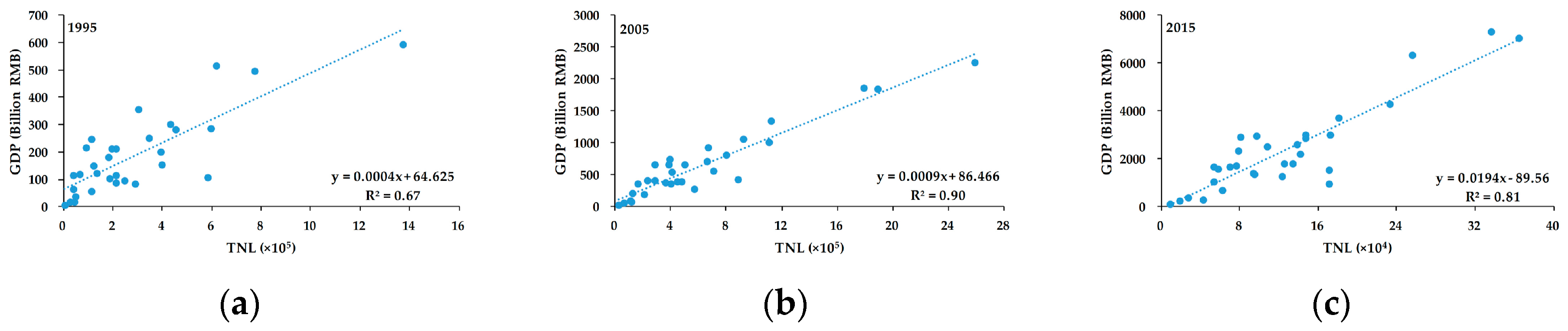
Figure 4.
Linear models between the statistical GDP data and TNL in provincial units at the country level: (a) the model for 1995 using DMSP-OLS data; (b) the model for 2005 using DMSP-OLS data; (c) the model for 2015 using NPP-VIIRS data.
Figure 4.
Linear models between the statistical GDP data and TNL in provincial units at the country level: (a) the model for 1995 using DMSP-OLS data; (b) the model for 2005 using DMSP-OLS data; (c) the model for 2015 using NPP-VIIRS data.

Figure 5.
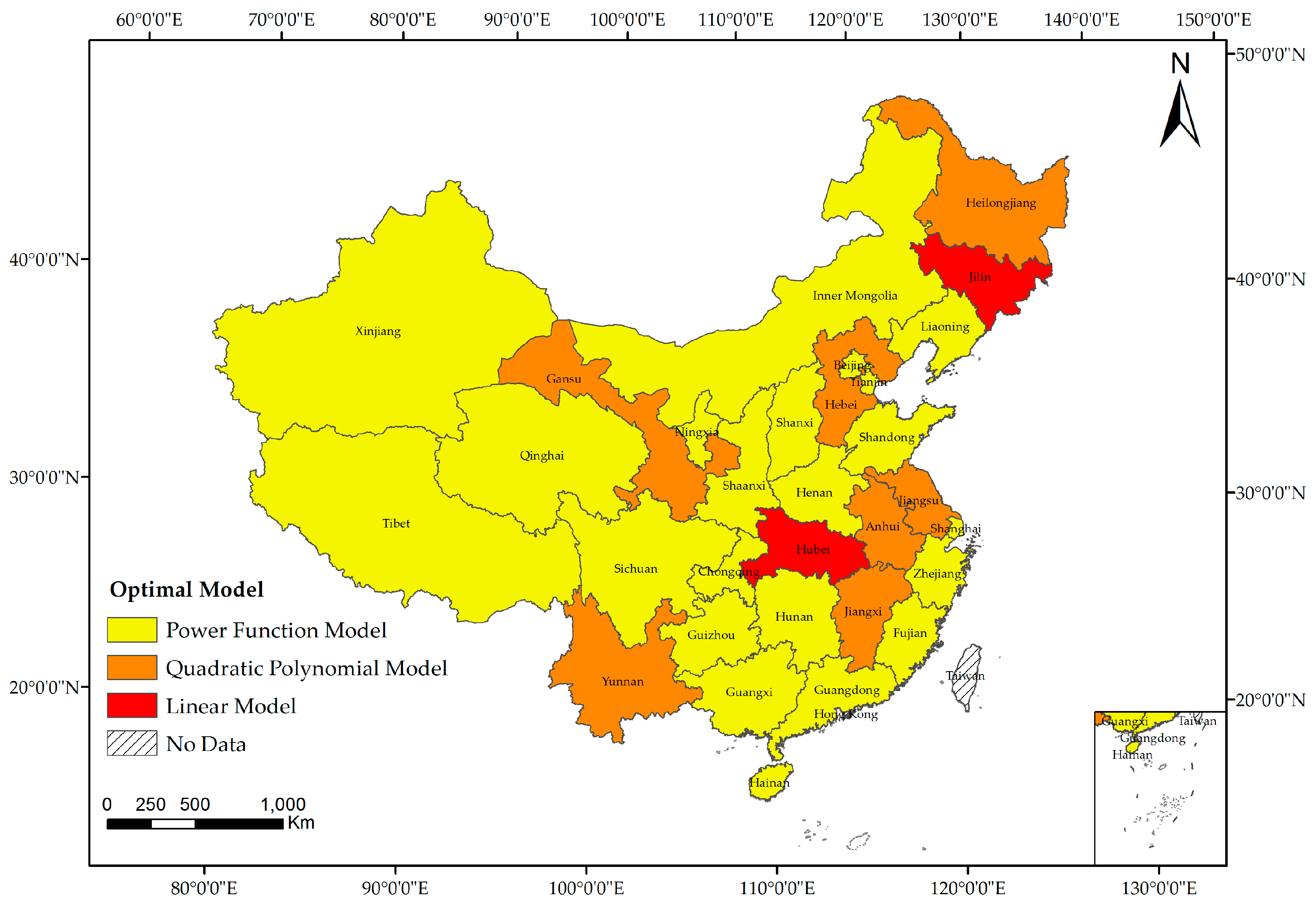
Spatial distribution of optimal models of the relationship between the statistical GDP data and TNL at the provincial level.
Figure 5.
Spatial distribution of optimal models of the relationship between the statistical GDP data and TNL at the provincial level.

Figure 6.
Optimal models of the relationship between the statistical GDP data and TNL for different provinces: (a) the linear model for Hubei; (b) the quadratic polynomial model for Gansu; (c) the power function model for Guangdong.
Figure 6.
Optimal models of the relationship between the statistical GDP data and TNL for different provinces: (a) the linear model for Hubei; (b) the quadratic polynomial model for Gansu; (c) the power function model for Guangdong.

Figure 7.
Spatial distribution of gaps in the growth rates between TNL and GDP at the provincial level.
Figure 7.
Spatial distribution of gaps in the growth rates between TNL and GDP at the provincial level.


Table 1.
Coefficients of the regression models for intercalibration.
| Satellite | Year | a | b | Satellite | Year | a | b |
|---|---|---|---|---|---|---|---|
| F10 | 1992 | 0.214 | 2.110 | F15 | 2001 | 0.197 | 2.155 |
| F10 | 1993 | 0.255 | 2.000 | F15 | 2002 | 0.206 | 2.105 |
| F10 | 1994 | 0.238 | 2.028 | F15 | 2003 | 0.329 | 1.845 |
| F12 | 1994 | 0.196 | 2.160 | F15 | 2004 | 0.321 | 1.842 |
| F12 | 1995 | 0.200 | 2.128 | F15 | 2005 | 0.283 | 1.916 |
| F12 | 1996 | 0.200 | 2.128 | F15 | 2006 | 0.288 | 1.898 |
| F12 | 1997 | 0.194 | 2.146 | F15 | 2007 | 0.294 | 1.887 |
| F12 | 1998 | 0.181 | 2.188 | F16 | 2004 | 0.233 | 2.024 |
| F12 | 1999 | 0.163 | 2.278 | F16 | 2005 | 0.268 | 1.934 |
| F14 | 1997 | 0.253 | 1.976 | F16 | 2006 | 0.256 | 1.965 |
| F14 | 1998 | 0.242 | 2.000 | F16 | 2007 | 0.219 | 2.049 |
| F14 | 1999 | 0.248 | 1.980 | F16 | 2008 | 0.226 | 2.033 |
| F14 | 2000 | 0.242 | 2.000 | F16 | 2009 | 0.216 | 2.083 |
| F14 | 2001 | 0.213 | 2.079 | F18 | 2010 | 0.154 | 2.326 |
| F14 | 2002 | 0.233 | 2.016 | F18 | 2011 | 0.201 | 2.132 |
| F14 | 2003 | 0.243 | 1.988 | F18 | 2012 | 0.185 | 2.169 |
| F15 | 2000 | 0.194 | 2.151 | F18 | 2013 | 0.185 | 2.165 |
Table 2.
Accuracy assessment of the TNL generated using NPP-VIIRS data and the TNL generated using DMSP-OLS data in 2012 and 2013.
Table 2.
Accuracy assessment of the TNL generated using NPP-VIIRS data and the TNL generated using DMSP-OLS data in 2012 and 2013.
| Province | 2012 | 2013 | ||||
|---|---|---|---|---|---|---|
| DMSP-OLS TNL | Extended TNL | RE (%) | DMSP-OLS TNL | Extended TNL | RE (%) | |
| Beijing | 868,571.94 | 869,042.45 | 0.05 | 905,903.10 | 951,355.48 | 5.02 |
| Tianjin | 703,545.22 | 746,497.03 | 6.11 | 768,575.13 | 835,504.21 | 8.71 |
| Hebei | 2,032,137.66 | 1,556,920.89 | −23.39 | 2,238,316.98 | 1,937,483.21 | −13.44 |
| Shanxi | 1,342,767.96 | 1,089,614.71 | −18.85 | 1,457,144.20 | 1,350,146.02 | −7.34 |
| Inner Mongolia | 1,317,047.05 | 1,015,907.00 | −22.86 | 1,409,399.81 | 1,232,594.12 | −12.54 |
| Liaoning | 1,491,362.08 | 1,532,125.78 | 2.73 | 1,596,523.05 | 1,724,975.76 | 8.05 |
| Jilin | 749,307.58 | 832,034.67 | 11.04 | 855,678.48 | 963,947.10 | 12.65 |
| Heilongjiang | 1,314,178.27 | 1,411,571.96 | 7.41 | 1,523,745.99 | 1,741,625.34 | 14.30 |
| Shanghai | 816,233.48 | 1,110,917.84 | 36.10 | 887,388.60 | 1,239,955.79 | 39.73 |
| Jiangsu | 3,680,608.49 | 3,509,035.95 | −4.66 | 4,308,393.36 | 4,096,784.55 | −4.91 |
| Zhejiang | 2,161,638.14 | 2,059,749.70 | −4.71 | 2,361,509.36 | 2,568,020.33 | 8.74 |
| Anhui | 1,079,116.60 | 1,085,624.14 | 0.60 | 1,346,950.22 | 1,450,477.27 | 7.69 |
| Fujian | 1,117,935.29 | 1,033,994.16 | −7.51 | 1,306,931.81 | 1,423,318.60 | 8.91 |
| Jiangxi | 477,494.68 | 364,004.28 | −23.77 | 635,416.26 | 517,184.56 | −18.61 |
| Shandong | 3,062,092.93 | 2,193,081.00 | −28.38 | 3,490,370.24 | 2,856,238.90 | −18.17 |
| Henan | 1,709,321.21 | 1,502,155.22 | −12.12 | 1,999,349.99 | 2,028,319.28 | 1.45 |
| Hubei | 723,142.54 | 644,961.65 | −10.81 | 1,023,120.28 | 968,570.70 | −5.33 |
| Hunan | 506,236.28 | 369,085.71 | −27.09 | 763,774.88 | 804,439.05 | 5.32 |
| Guangdong | 3,579,626.22 | 3,479,545.87 | −2.80 | 3,970,102.44 | 3,890,371.65 | −2.01 |
| Guangxi | 586,690.31 | 401,061.07 | −31.64 | 707,193.83 | 810,857.53 | 14.66 |
| Hainan | 259,255.69 | 232,785.55 | −10.21 | 283,777.66 | 257,632.97 | −9.21 |
| Chongqing | 342,311.97 | 319,365.17 | −6.70 | 430,971.42 | 488,065.43 | 13.25 |
| Sichuan | 804,809.15 | 1,059,718.49 | 31.67 | 1,098,418.44 | 1,452,896.88 | 32.27 |
| Guizhou | 261,801.09 | 324,743.63 | 24.04 | 411,543.14 | 654,998.85 | 59.16 |
| Yunnan | 890,418.66 | 854,610.21 | −4.02 | 970,447.49 | 1,017,251.10 | 4.82 |
| Tibet | 54,268.23 | 64,777.11 | 19.36 | 59,741.55 | 74,223.86 | 24.24 |
| Shaanxi | 1,111,777.06 | 1,124,106.54 | 1.11 | 1,263,576.61 | 1,409,005.17 | 11.51 |
| Gansu | 498,009.42 | 448,341.41 | −9.97 | 578,400.64 | 574,393.24 | −0.69 |
| Qinghai | 158,669.97 | 135,821.67 | −14.40 | 178,478.81 | 172,379.87 | −3.42 |
| Ningxia | 310,587.95 | 272,089.48 | −12.40 | 337,160.76 | 359,709.51 | 6.69 |
| Xinjiang | 1,101,950.18 | 1,235,927.81 | 12.16 | 1,235,204.49 | 1,471,523.52 | 19.13 |
| MARE (%) | − | − | 13.83 | − | − | 12.97 |
Table 3.
Different categories of extension accuracies for TNL at the provincial level.
| Year | Percentage of Absolute RE (%) | ||
|---|---|---|---|
| High Accuracy (%) | Moderate Accuracy (%) | Inaccuracy (%) | |
| 2012 | 83.87 | 16.13 | 0.00 |
| 2013 | 90.32 | 6.45 | 3.23 |
Table 4.
Accuracy assessment of the GDP estimated using a linear model in time series and linear models in provincial units at the country level from 1992 to 2015.
Table 4.
Accuracy assessment of the GDP estimated using a linear model in time series and linear models in provincial units at the country level from 1992 to 2015.
| Year | Statistical GDP (Billion RMB) | Modeling in Time Series | Modeling in Provincial Units | |||
|---|---|---|---|---|---|---|
| Estimated GDP (Billion RMB) | RE (%) | Estimated GDP (Billion RMB) | RE (%) | R2 | ||
| 1992 | 2719.45 | 2436.05 | −10.42 | 1916.55 | −29.52 | 0.56 |
| 1993 | 3567.32 | 3952.71 | 10.80 | 2233.19 | −37.40 | 0.65 |
| 1994 | 4863.75 | 5637.04 | 15.90 | 2851.05 | −41.38 | 0.64 |
| 1995 | 6133.99 | 6646.20 | 8.35 | 3898.66 | −36.44 | 0.67 |
| 1996 | 7181.36 | 6896.10 | −3.97 | 4531.75 | −36.90 | 0.66 |
| 1997 | 7971.50 | 7371.36 | −7.53 | 5116.33 | −35.82 | 0.68 |
| 1998 | 8519.55 | 8392.86 | −1.49 | 5777.19 | −32.19 | 0.71 |
| 1999 | 9056.44 | 8936.78 | −1.32 | 6276.96 | −30.69 | 0.73 |
| 2000 | 10,028.01 | 10,413.99 | 3.85 | 7113.27 | −29.07 | 0.75 |
| 2001 | 11,086.31 | 11,724.99 | 5.76 | 8109.49 | −26.85 | 0.77 |
| 2002 | 12,171.74 | 15,158.81 | 24.54 | 9997.43 | −17.86 | 0.85 |
| 2003 | 13,742.20 | 18,636.02 | 35.61 | 11,487.16 | −16.41 | 0.88 |
| 2004 | 16,184.02 | 21,122.73 | 30.52 | 14,319.63 | −11.52 | 0.88 |
| 2005 | 18,731.89 | 22,111.01 | 18.04 | 17,517.64 | −6.48 | 0.90 |
| 2006 | 21,943.85 | 25,153.04 | 14.62 | 20,978.78 | −4.40 | 0.91 |
| 2007 | 27,023.23 | 27,015.07 | −0.03 | 25,342.82 | −6.22 | 0.91 |
| 2008 | 31,951.55 | 28,151.61 | −11.89 | 29,321.33 | −8.23 | 0.89 |
| 2009 | 34,908.14 | 30,168.28 | −13.58 | 32,669.75 | −6.41 | 0.86 |
| 2010 | 41,303.03 | 37,571.10 | −9.04 | 39,417.30 | −4.57 | 0.88 |
| 2011 | 48,930.06 | 42,197.08 | −13.76 | 45,750.55 | −6.50 | 0.88 |
| 2012 | 54,036.74 | 45,448.23 | −15.89 | 50,701.78 | −6.17 | 0.86 |
| 2013 | 59,524.44 | 53,284.03 | −10.48 | 57,181.25 | −3.94 | 0.88 |
| 2014 | 64,397.40 | 68,086.46 | 5.73 | 70,282.66 | 9.14 | 0.82 |
| 2015 | 68,550.58 | 78,015.00 | 13.81 | 75,757.34 | 10.51 | 0.81 |
| MARE (%) | − | − | 11.96 | − | 18.94 | − |
Table 5.
Model fitting precision values at the provincial level.
| Province | Linear | Quadratic | Power | |||
|---|---|---|---|---|---|---|
| R2 | MARE (%) | R2 | MARE (%) | R2 | MARE (%) | |
| Beijing | 0.93 | 51.00 | 0.99 | 11.55 | 0.99 | 10.94 |
| Tianjin | 0.96 | 53.69 | 0.99 | 12.15 | 0.99 | 7.91 |
| Hebei | 0.99 | 16.06 | 0.99 | 8.43 | 0.99 | 9.52 |
| Shanxi | 0.96 | 36.28 | 0.96 | 31.85 | 0.96 | 16.90 |
| Inner Mongolia | 0.99 | 15.97 | 0.99 | 18.94 | 0.98 | 15.28 |
| Liaoning | 0.98 | 12.84 | 0.98 | 12.59 | 0.97 | 11.28 |
| Jilin | 0.95 | 16.41 | 0.98 | 20.85 | 0.95 | 17.93 |
| Heilongjiang | 0.92 | 22.12 | 0.97 | 13.64 | 0.92 | 19.63 |
| Shanghai | 0.89 | 20.19 | 0.91 | 27.32 | 0.94 | 20.05 |
| Jiangsu | 0.98 | 19.89 | 0.99 | 12.68 | 0.97 | 13.34 |
| Zhejiang | 0.97 | 18.46 | 0.97 | 15.31 | 0.97 | 13.28 |
| Anhui | 0.97 | 20.33 | 0.99 | 11.35 | 0.96 | 15.34 |
| Fujian | 0.98 | 13.39 | 0.98 | 23.85 | 0.98 | 10.87 |
| Jiangxi | 0.95 | 24.98 | 0.96 | 23.46 | 0.93 | 23.95 |
| Shandong | 0.94 | 34.92 | 0.97 | 12.74 | 0.98 | 12.65 |
| Henan | 0.98 | 15.87 | 0.98 | 16.45 | 0.98 | 12.25 |
| Hubei | 0.95 | 16.89 | 0.96 | 25.38 | 0.95 | 17.00 |
| Hunan | 0.93 | 23.29 | 0.94 | 28.08 | 0.93 | 22.91 |
| Guangdong | 0.94 | 45.17 | 0.97 | 17.53 | 0.98 | 11.98 |
| Guangxi | 0.97 | 16.67 | 0.97 | 21.14 | 0.97 | 13.00 |
| Hainan | 0.98 | 13.60 | 0.98 | 12.34 | 0.99 | 7.76 |
| Chongqing | 0.94 | 21.25 | 0.96 | 27.61 | 0.94 | 19.86 |
| Sichuan | 0.90 | 32.38 | 0.96 | 27.32 | 0.95 | 19.15 |
| Guizhou | 0.92 | 35.19 | 0.97 | 25.73 | 0.95 | 19.81 |
| Yunnan | 0.98 | 21.45 | 0.99 | 10.35 | 0.98 | 10.46 |
| Tibet | 0.97 | 16.67 | 0.97 | 25.67 | 0.98 | 12.58 |
| Shaanxi | 0.98 | 11.92 | 0.98 | 21.00 | 0.98 | 10.93 |
| Gansu | 0.96 | 22.42 | 0.99 | 13.83 | 0.94 | 19.75 |
| Qinghai | 0.98 | 13.29 | 0.99 | 17.91 | 0.98 | 12.25 |
| Ningxia | 0.96 | 16.30 | 0.98 | 23.97 | 0.97 | 16.12 |
| Xinjiang | 0.88 | 31.73 | 0.96 | 36.76 | 0.94 | 17.58 |
| Mean | 0.95 | 23.57 | 0.97 | 19.61 | 0.96 | 14.91 |
© 2017 by the authors. Licensee MDPI, Basel, Switzerland. This article is an open access article distributed under the terms and conditions of the Creative Commons Attribution (CC BY) license (http://creativecommons.org/licenses/by/4.0/).
Share and Cite
MDPI and ACS Style
Zhu, X.; Ma, M.; Yang, H.; Ge, W. Modeling the Spatiotemporal Dynamics of Gross Domestic Product in China Using Extended Temporal Coverage Nighttime Light Data. Remote Sens. 2017, 9, 626. https://doi.org/10.3390/rs9060626
AMA Style
Zhu X, Ma M, Yang H, Ge W. Modeling the Spatiotemporal Dynamics of Gross Domestic Product in China Using Extended Temporal Coverage Nighttime Light Data. Remote Sensing. 2017; 9(6):626. https://doi.org/10.3390/rs9060626
Chicago/Turabian StyleZhu, Xiaobo, Mingguo Ma, Hong Yang, and Wei Ge. 2017. "Modeling the Spatiotemporal Dynamics of Gross Domestic Product in China Using Extended Temporal Coverage Nighttime Light Data" Remote Sensing 9, no. 6: 626. https://doi.org/10.3390/rs9060626
Note that from the first issue of 2016, this journal uses article numbers instead of page numbers. See further details here.