Monitoring of Wheat Growth Status and Mapping of Wheat Yield’s within-Field Spatial Variations Using Color Images Acquired from UAV-camera System

Abstract

Applications of remote sensing using unmanned aerial vehicle (UAV) in agriculture has proved to be an effective and efficient way of obtaining field information. In this study, we validated the feasibility of utilizing multi-temporal color images acquired from a low altitude UAV-camera system to monitor real-time wheat growth status and to map within-field spatial variations of wheat yield for smallholder wheat growers, which could serve as references for site-specific operations. Firstly, eight orthomosaic images covering a small winter wheat field were generated to monitor wheat growth status from heading stage to ripening stage in Hokkaido, Japan. Multi-temporal orthomosaic images indicated straightforward sense of canopy color changes and spatial variations of tiller densities. Besides, the last two orthomosaic images taken from about two weeks prior to harvesting also notified the occurrence of lodging by visual inspection, which could be used to generate navigation maps guiding drivers or autonomous harvesting vehicles to adjust operation speed according to specific lodging situations for less harvesting loss. Subsequently orthomosaic images were geo-referenced so that further study on stepwise regression analysis among nine wheat yield samples and five color vegetation indices (CVI) could be conducted, which showed that wheat yield correlated with four accumulative CVIs of visible-band difference vegetation index (VDVI), normalized green-blue difference index (NGBDI), green-red ratio index (GRRI), and excess green vegetation index (ExG), with the coefficient of determination and RMSE as 0.94 and 0.02, respectively. The average value of sampled wheat yield was 8.6 t/ha. The regression model was also validated by using leave-one-out cross validation (LOOCV) method, of which root-mean-square error of predication (RMSEP) was 0.06. Finally, based on the stepwise regression model, a map of estimated wheat yield was generated, so that within-field spatial variations of wheat yield, which was usually seen as general information on soil fertility, water potential, tiller density, etc., could be better understood for applications of site-specific or variable-rate operations. Average yield of the studied field was also calculated according to the map of wheat yield as 7.2 t/ha.

1. Introduction

Remote sensing has been successfully used as an effective method for obtaining field information through analysis of reflectance or radiance of specific bands’ digital numbers [1,2]. According to different types of platforms, agricultural remote sensing could generally be categorized into satellite remote sensing, aerial remote sensing, and near-ground remote sensing. Multi-spectral satellite imagery has long been applied to detect vegetation areas, monitor crop growth status, and estimate crop yield, etc., in large scale [3,4]. Aerial remote sensing using aircrafts or balloon has been introduced as supplementary method and often carried out as one-time operations. Aerial photography has been used to monitor crop growth status as regional or medium-scale applications of agricultural remote sensing ever since 1950s by using color or color-infrared cameras [5]. Near-ground agricultural remote sensing is often referred to as frame-based or pillar-based applications [6]. Recently, the cutting edge application of small fixed- and/or rotary-wing unmanned aerial vehicles (UAV) for spatial sampling or preliminary mapping for variable-rate operations has begun, since UAV imagery may be acquired more cost-effectively, with excellent maneuverability as well as increasing spatial resolution, and with greater safety when compared with manned aircraft [7,8,9]. Agricultural application of UAV remote sensing by using color cameras instantly provides researchers and farmers with actual and intuitive visualization of crop growth status, since color images accentuate particular vegetation greenness and have been suggested to be less sensitive to variations of illumination conditions [10,11]. Meanwhile, the application of color cameras also sharply decreases the high cost of remote sensing [12], since most digital cameras use a Bayer-pattern array of filters to obtain an RGB digital image, and the acquisition of near-infrared (NIR) band images usually requires an extra filter that converts digital numbers of either blue or red light in Bayer array into NIR readings through massive post-processing and calibration work [13]. Rasmussen et al. investigated the reliability of four different vegetation indices derived from consumer-grade true color camera as well as a color-infrared camera that are mounted on UAVs for assessing experimental plots, and concluded that vegetation indices of UAV imagery have the same ability as ground-based recordings to quantify crop responses to experimental treatments, although such shortcomings like angular variations in reflectance, stitching, and ambient light fluctuation should be taken into consideration [14]. Torres-Sánchez et al. mapped multi-temporal vegetation fraction in early-season wheat fields by using a UAV equipped with commercial color camera and studied the influence of flight altitude and days after sowing on the classification accuracy, which showed that visible spectral vegetation indices derived from low-altitude UAV-camera system could be used as a suitable tool to discriminate vegetation in wheat fields in the early season [15]. Woebbecke et al. tested several color indices derived using chromatic coordinates and modified hue to distinguish vegetation from background such as bare soil and crop residues [16], among which the excess green vegetation index (ExG) provides a near-binary intensity image outlining a plant region of interest has been widely cited. Cui et al. evaluated the reliability of using color digital images to estimate above ground biomass at canopy level of winter wheat by taking pictures from one meter above the top of the wheat canopy [17]. In short, most past agricultural studies on color images focused on individual level of crop or weed, and the point-source samplings of which are usually inevitably both time-consuming and have to be conducted under poor working condition.

Wheat (Triticum spp., or Triticum aestivum L.) has been among the most produced cereal grains for a long time. In 2009, global wheat production reached about 680 million tons, which made it the second most produced cereal grain after maize [18]. In order to optimize wheat yield and grain quality, especially in terms of protein content that varies significantly depending on different agricultural practices, optimal agronomic management in accordance with wheat development stages is critical. It requires that farmers have a detailed understanding of wheat growth status during each specific development stage in wheat cultivation [19], which indicates that real-time monitoring of actual wheat growth status throughout the wheat growing season is of vital importance in helping wheat growers with management decision making. Meanwhile, it was frequently reported that reproductive growth of wheat after the flowering stage is closely related to grain yield, and many studies in recent years on wheat growth have indicated that accumulative NDVI values of multi-temporal satellite remote sensing images after flowering stage have good relationship with crop yield [2,20]. Therefore, in this study, eight-color orthomosaic images acquired from a low altitude UAV-camera system were used to intuitively monitor and assess overall growth status of a winter wheat field from heading stage to ripening stage from early June to the end of July 2015 at the interval of about one week in Hokkaido, Japan. A multivariate analysis of field samples of wheat yield and accumulative CVIs derived from orthomosaic images was performed to estimate wheat yield. Subsequently, an original method of mapping wheat yields within-field spatial variations was proposed to provide reference for decision making in terms of site-specific agriculture based on the result of regression model.

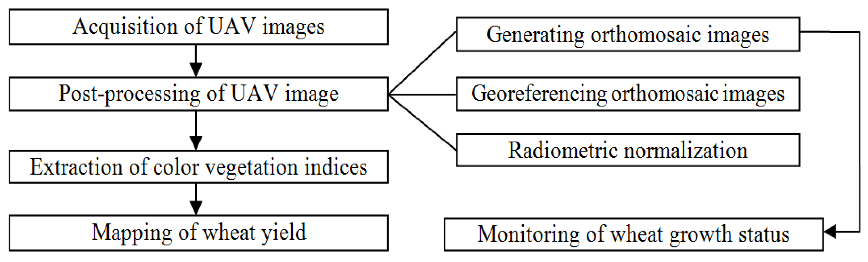
2. Materials and Methods

The overall approach of this proposed method of monitoring wheat growth status as, well as mapping within-field wheat yield’s spatial variations, consists of four key steps: acquisition of high resolution UAV photographs using the low altitude UAV-camera system; post-processing of UAV images including orthomosaicking, georeferencing, and radiometric normalization; extraction of color vegetation indices from post-processed othomosaic images; and mapping of with-field wheat yield’s spatial variations through multivariate analysis between color vegetation indices and sampled grain yields, shown in Figure 1. This study adopted World Geodetic System 1984, or WGS84, as the coordinate system for geo-referenced images, maps, or any coordinates used in this paper if not particularly indicated.

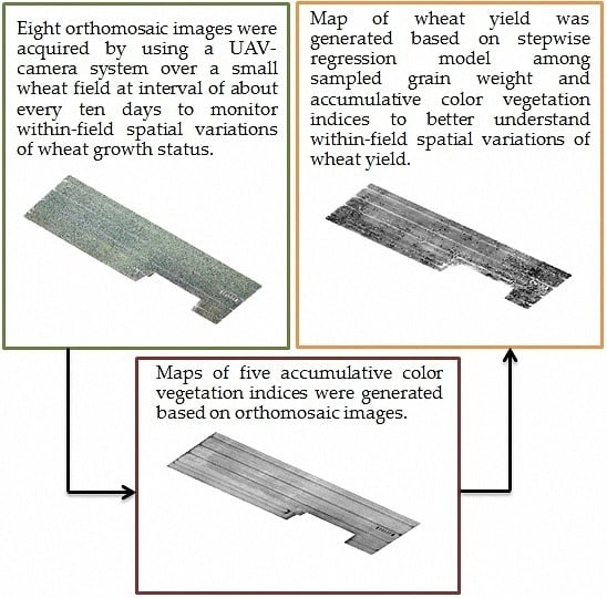
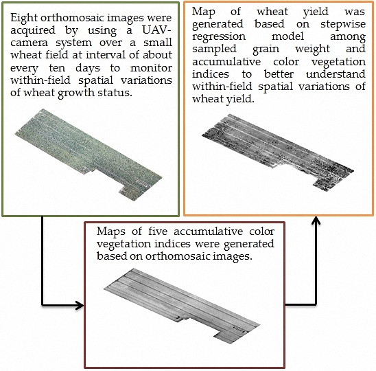
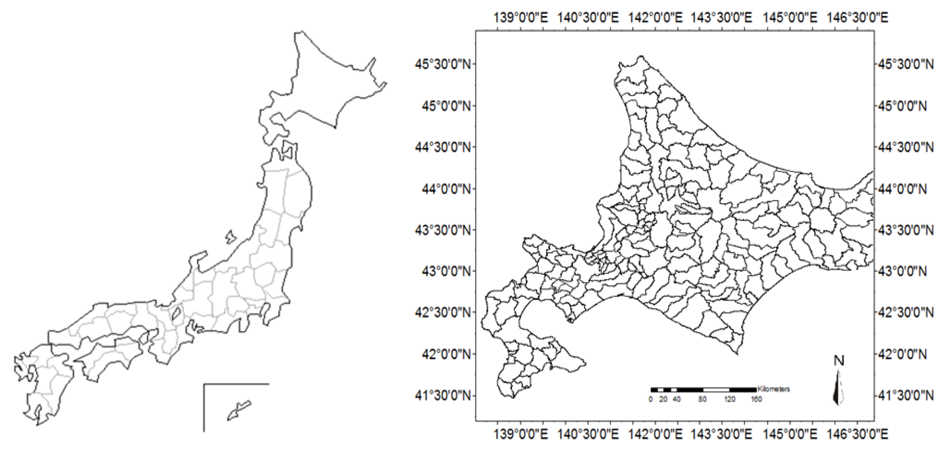
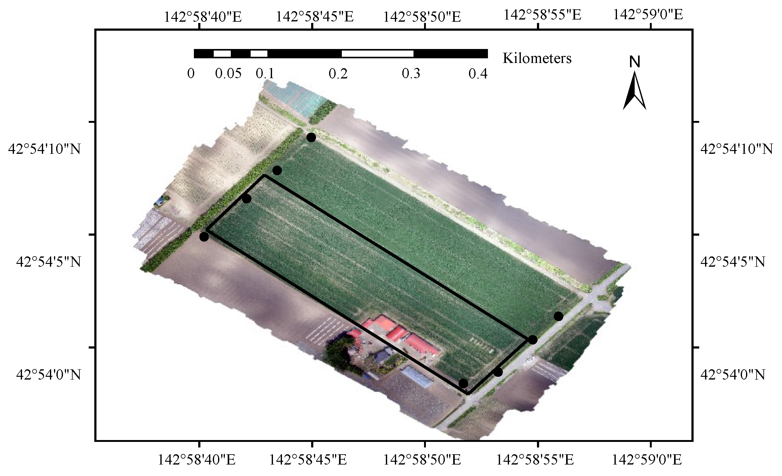
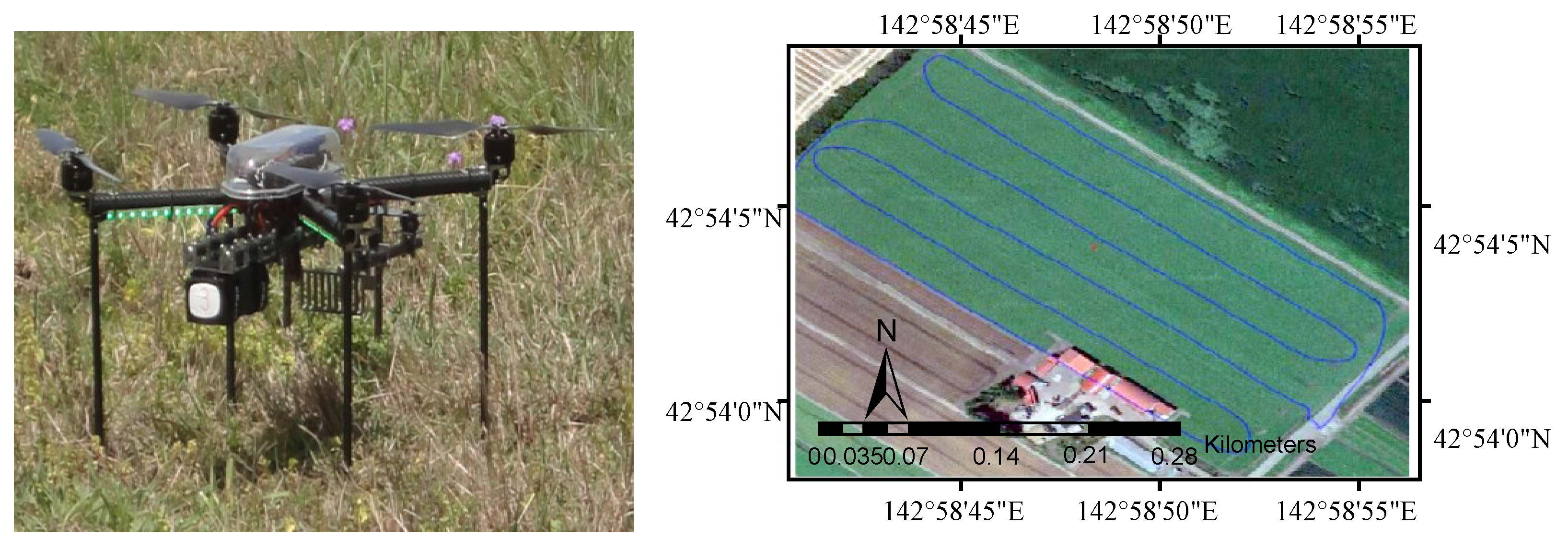
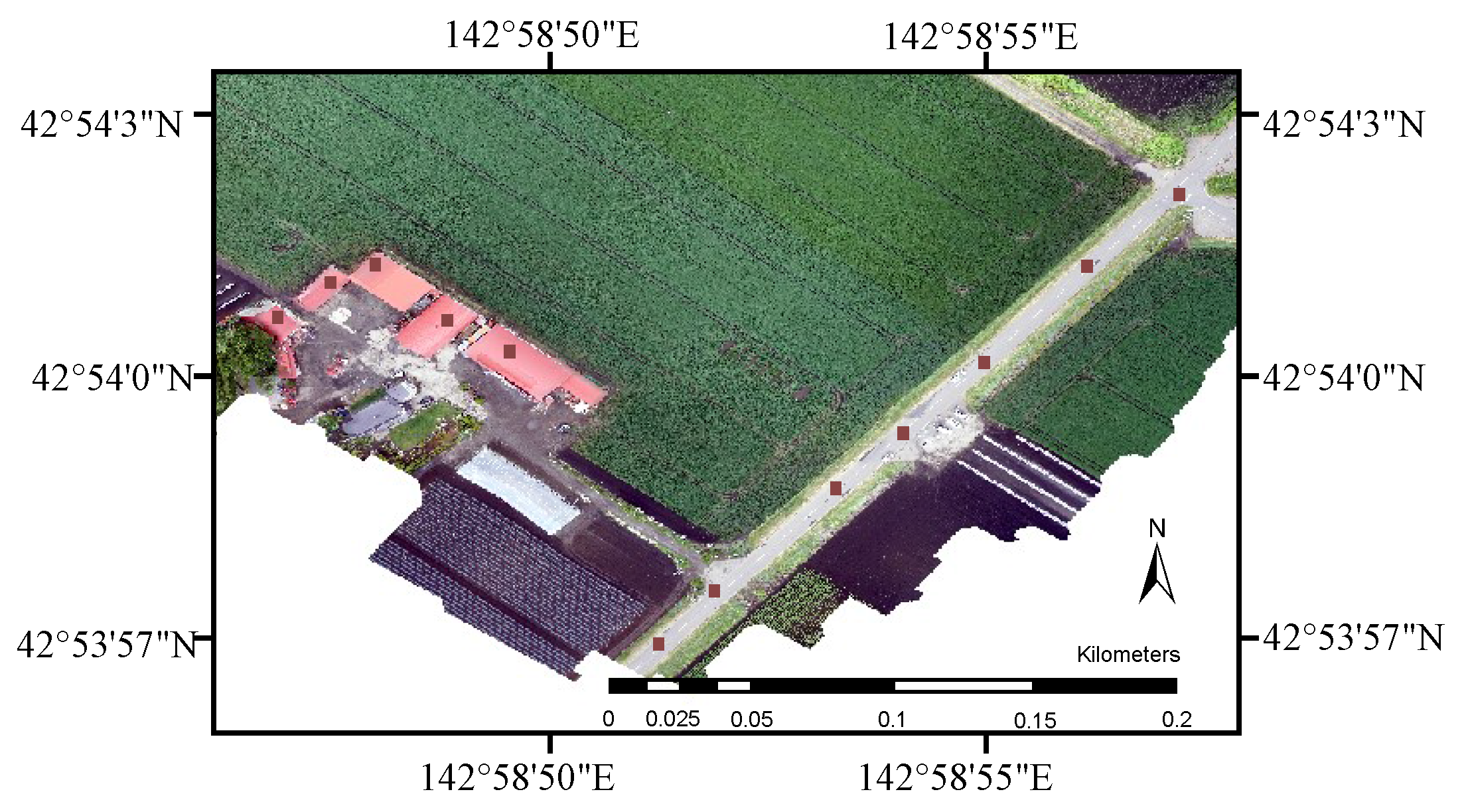
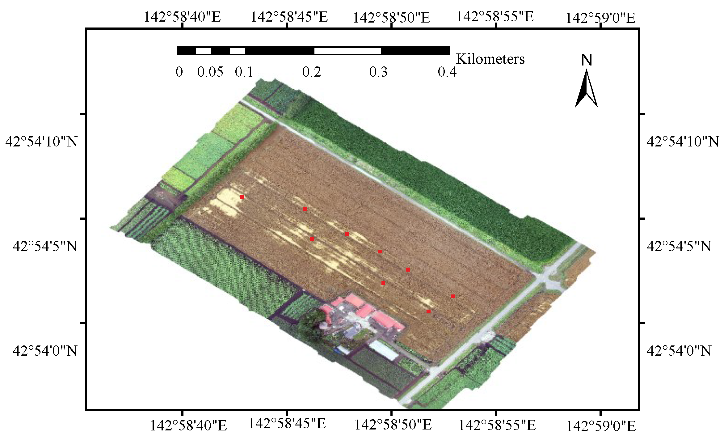
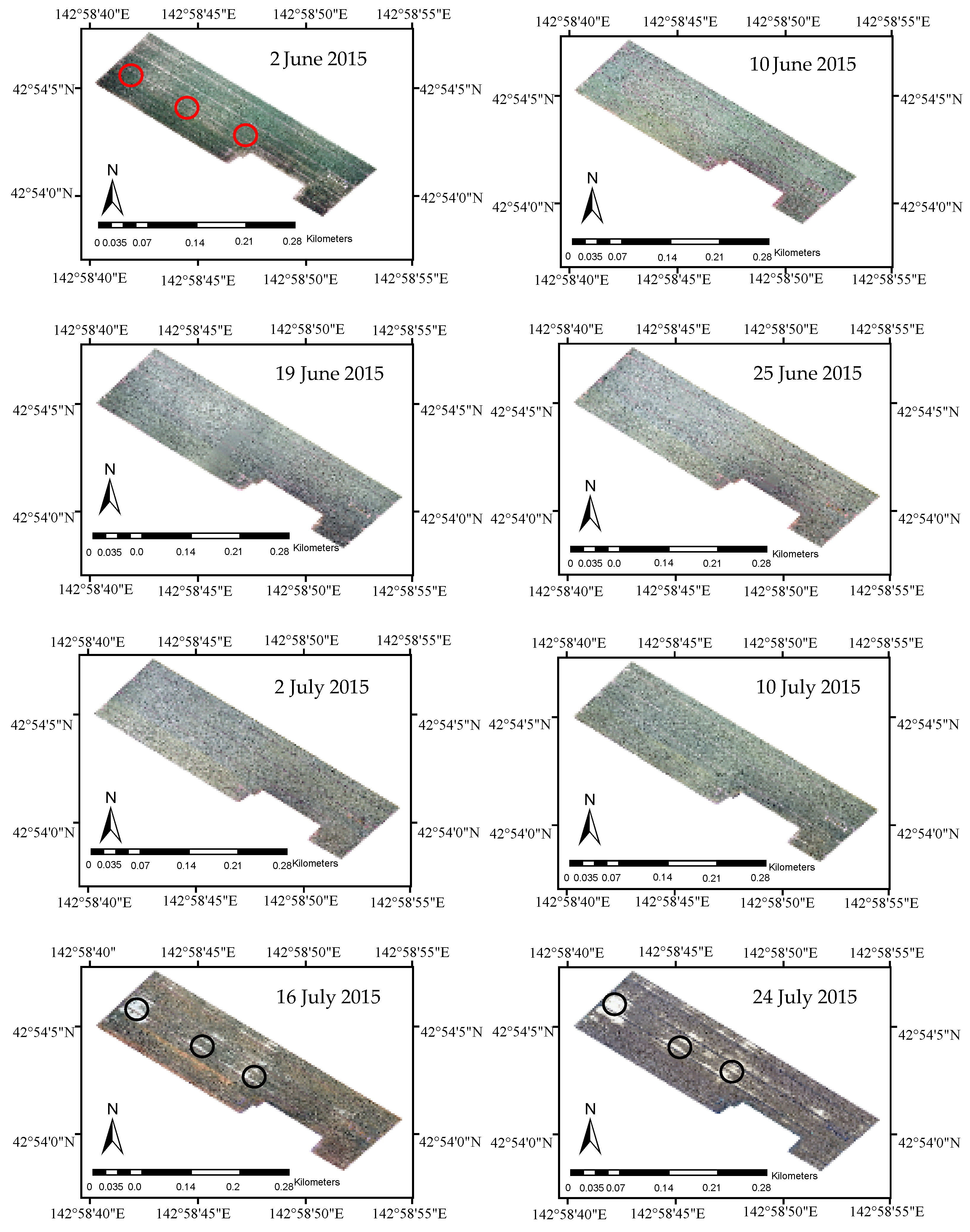
2.1. Field Site and Acquisition of UAV Images

Experiments were established on a winter wheat farmland located in Memuro, Hokkaido, Japan (around 42.902041°N–42.899607°N and 142.977953°E–142.981734°E), shown in Figure 2. The lower left field (marked in black rectangle shown in Figure 3) was planted with the winter wheat variety of Kitahonami, occupying about 3.2 ha., which is the most widely planted winter wheat variety in Hokkaido and is reported to have taken up about 90% acreages of winter wheat in Hokkaido alone [21]. The wheat field was planted around 25 September 2014 and harvested on 27 July 2015. Nine grain samples of Kitahonami were taken on 24 July 2015, three days prior to harvesting, and the position of each yield sample was measured by using Trimble SPS855 GNSS modular receiver in RTK-GPS mode with horizontal positioning accuracy of 8 mm [22]. Regional annual precipitation of this area is around 957.3 mm, with average annual temperature of 6.1 °C [23].

In this experiment, a small quadrotor (ENROUTE CO., LTD., Fujimino, Japan), shown in Figure 4, was used as the platform of low altitude (about 100 m above ground level) UAV-camera system, and its performance parameters were listed in

Table 1. Performance parameters of UAV-camera system.

UAV Specification		Camera Specification
Overall diameter × height (mm)	φ1009 × 254	Weight (gram)	345
Rated operation weight (kg)	3.2	Camera resolution	4000 × 6000 pixels
Endurance (min)	15–20	Focal length (mm)	16
Range (km)	10	Sensor size(mm)	23.5 × 15.6
Maximus flying altitude (m)	250

. A laptop installed with Ground Controlling Station (GCS) software was used to monitor and control the autonomous UAV flight through telemetry radio. Autonomous flights were conducted eight times at the interval of about one week from winter wheat’s heading stage to ripening stage, on 2, 10, 19, and 25 June 2015, and 2, 10, 16, and 24 July 2015 (at about 11:00 local time), using the flight paths that were designed beforehand in the GCS software, shown in Figure 4 as blue lines.

A SONY ILCE-6000 commercial digital camera was used to take pictures in continuous mode every two seconds (f/8, 1/500 sec, ISO 100), and the camera specification was also described in Table 1. During each flight, the camera was fixed on a two-axis gimbal, pointing vertically downwards and took about 120 photos covering two adjacent fields in order to get enough ground control points (GCPs) for georeferrencing the orthomosaic images in post-processing. The ground resolution of these pictures was about 2.5 cm. Every 120 individual photographs were stitched together as an orthomosaic image by using Agisoft Photoscan software (Agisoft LLC, Petersburg, Russia), which was shown in Figure 3. Each of the orthomosaic images have about 3600 × 2450 pixels in size, and the ground resolution reached up to about 12.5 cm after orthomosaicking.

Georeferencing, or geocoding, is the process of assigning geographic coordinates to data (usually an image file) that are spatial in nature but have no explicit geographic coordinates (for example aerial photographs). It is necessary to georeference such images so that thereafter they can be further studied using geographic information system (GIS) technology. The georeferencing process of the orthomosaic images was accomplished using ArcMap 10.2 (ESRI Inc., Redlands, AB, Canada) software by adopting the 1st order polynomial transformation method and taking eight wheat row corners that dispersed around the field as ground controlling points (GCP). The transformation created two least-square-fit equations by comparing the image space coordinates of the GCPs with the geographic coordinates (latitude and longitude) and translated the image coordinates of each pixel into geographic coordinates. These GCPs’ geo-spatial coordinates were measured by using a Trimble SPS855 GNSS modular receiver in RTK-GPS mode.

2.2. Radiometric Normalization of Multi-Temporal UAV Images

Due to different illuminative situations, radiometric accuracy and consistency are difficult to maintain among multi-temporal remote sensing images. Relative radiometric correction, or radiometric normalization, was usually necessary to adjust multi-temporal remote sensing images to a set of reference data and compensate for the radiometric effects. In this paper, the pseudo-invariant features (PIF) method, which refers to ground objects whose reflectance values are nearly constant over time during a certain period [24], was used to perform radiometric normalization of these UAV orthomosaic images, band by band, respectively. Seven places along the road and five places on the roof were selected as PIFs in each othomosaic images. Around each PIF’s location, mean value of pixels distributed within the area of about 0.25 m² were calculated in each orthomosaic image, so that the influence of abnormal values caused by foreign matters etc. could be decreased. Subsequently, according to the PIFs’ values extracted from eight orthomosaic images taken on different dates, radiometric normalization models were built by performing linear regressions, taking the PIFs’ values extracted from each orthomosaic image as predictive terms and reference data as response variable. The reference data were generated by averaging each PIF’s multi-temporal pixel values of blue band, green band, and red band, respectively. The spatial distribution of the UAV images’ PIFs was shown as dark dots on the roof and road in Figure 5.

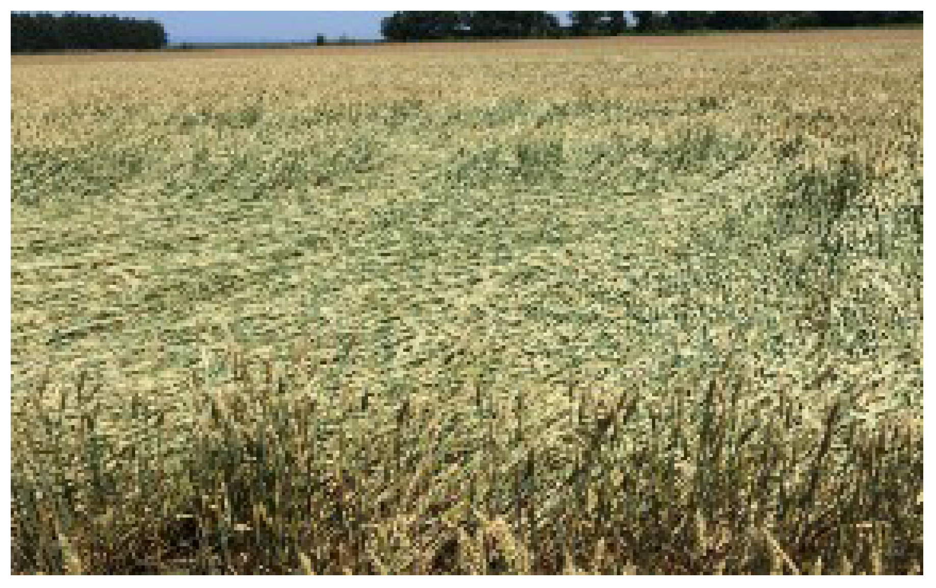
2.3. Field Sampling of Wheat Yield

Nine samples of wheat yield were measured by using a 1 m × 1 m square frame to separate samples of wheat canopies. Samples were selected after detailed visual inspection on eight orthomosaic images and field survey on the sampling day in order to representatively choose three samples of or nearby lodging area and six samples out of normal areas, of which the most flourished areas and sparse areas were both taken into consideration. Samples’ spatial distribution was shown in Figure 6. The sampling operation was conducted at 24 July 2015, three days ahead of harvesting, by collecting wheat ears within the specified 1-square-meter section. These samples’ geo-coordinates were acquired by using Trimble SPS855 GNSS modular receiver in RTK-GPS mode. After threshing, grain weight of each sample was calculated and converted to 12.5% moisture, listed in

Table 2. Samples of wheat yield.

Wheat Variety	Sample ID.	Sample Position		Sampled Grain Weight (kg, Converted to 12.5% Moisture)
		Latitude	Longitude
Kitahonami	1	42.901657	142.978642	1.01
	2	42.901097	142.979570	0.86
	3	42.900532	142.980497	0.84
	4	42.900180	142.981070	0.91
	5	42.900360	142.981302	0.85
	6	42.900694	142.980759	0.79
	7	42.900972	142.980286	0.82
	8	42.901202	142.979924	0.80
	9	42.901476	142.979472	0.83

.

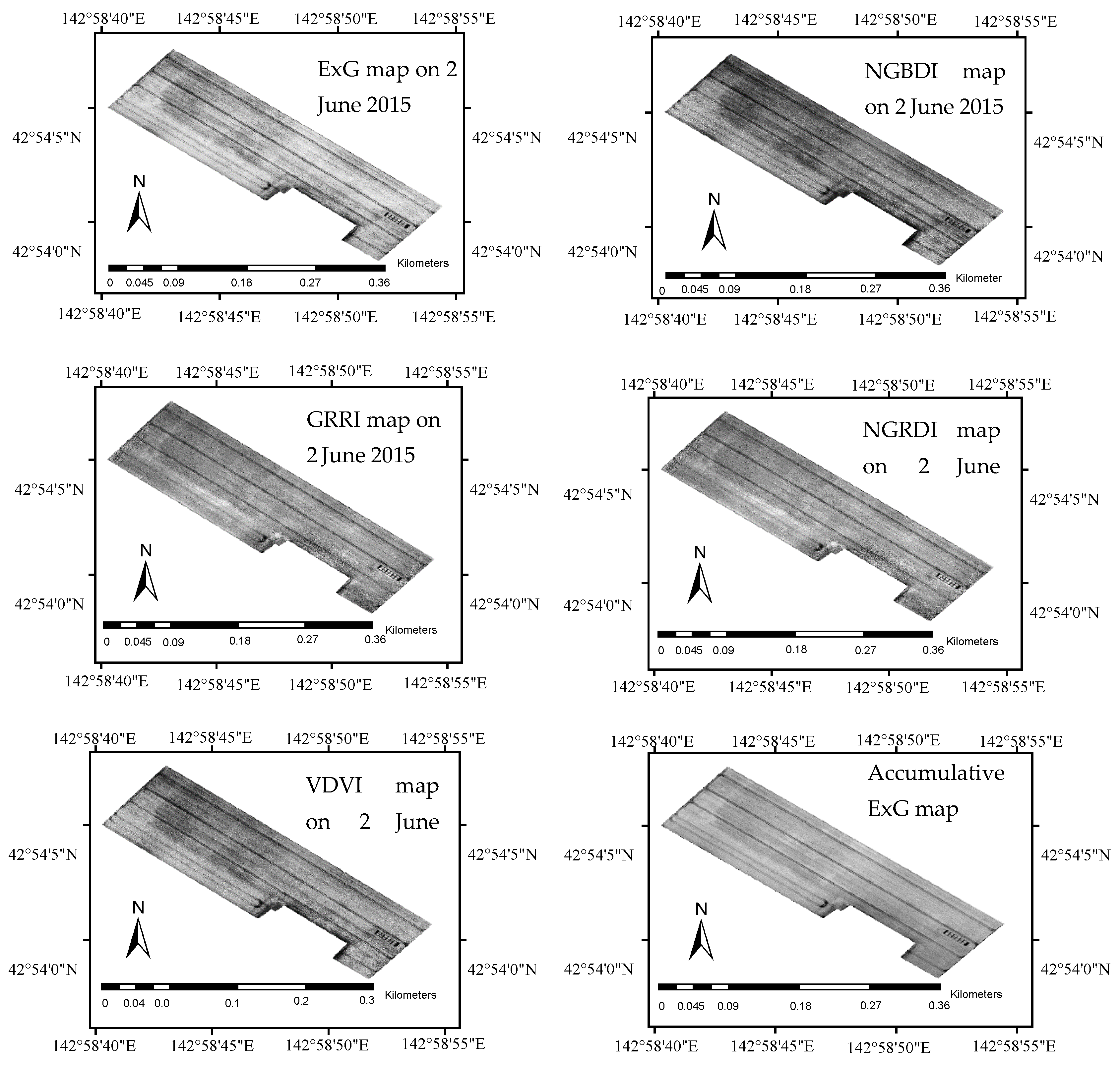
2.4. Generating CVI Maps Based on UAV Images

Vegetation index map refers to as a scalar image in which each pixel has only one single brightness value. The pixel values are often calculated from reflectance or radiance of specific bands of remote sensing images. In recent years, several CVIs based on color images that are different from the NDVI associated with near-infrared band were proposed to identify vegetative features such as ExG mentioned above. Other CVIs were also introduced in this study, including visible-band difference vegetation index (VDVI) [11], normalized green-red difference index (NGRDI) [25], normalized green-blue difference index (NGBDI) [11], green-red ratio index (GRRI) [26], and ExG [16], which were expressed respectively in the following equations:

VDVI = (2G − B − R)/(2G + B + R)

(1)

NGRDI = (G − R)/(G + R)

(2)

NGBDI =(G − B)/(G + B)

(3)

GRRI = G/R

(4)

ExG = 2G − B − R

(5)

where B, G, R denotes the radiometric normalized pixel values of each orthomosaic images’ blue, green, and red band, respectively.

Accordingly, orthomosaic images taken on eight different dates were all used to generate CVI maps of ExG, NGBDI, GRRI, NGRDI, and VDVI as scalar images by using ENVI software (Exelis VIS, Inc., Boulder, CO, USA), in which each pixel was determined from its existing multi-band radiometric normalized pixel values and using band math functions. Figure 7 illustrates examples of CVI maps based on orthomosaic images taken on 2 June 2015, as well as the accumulative ExG map, whilst CVI maps based on other orthomosaic images and accumulative CVI maps were omitted here due to limited space. The accumulative CVI maps were acquired, respectively, by overlapping each corresponding CVI maps and adding pixel values of these scalar images on different dates point for point. After applying a mean filter of 7 × 7 pixels (which covers about 1-square-meter area) to the accumulative CVI maps, brightness values of pixels that have the same geo-spatial coordinates with the nine wheat samples were extracted out of each accumulative CVI map. The extracted accumulative CVI values were used to conduct stepwise regression analysis with sampled wheat yield data. Then, according to the regression model among wheat yield data and values of accumulative CVIs, yield map was generated accordingly.

3. Result and Discussion

3.1. Monitoring of Wheat Growth Status

From multi-temporal UAV orthomosaic images (shown in Figure 8), we can get a straightforward visualization of the rapid change of wheat growth status through image interpretation. We can see that canopy greenness reached peak condition on 10 July 2015 and the process of yellowing began thereafter. We can also see within-field variation of wheat tiller densities, especially from early stage of wheat growth, from the image taken on 2 June 2015. To be specific, the areas circled in red had relatively higher level of tiller densities, which compounded with other environmental influences such as rainfall, wind, etc. and caused occurrence of lodging before harvesting when over-luxuriant canopies failed to support heavy wheat ears (see images from 16 July and 24 July, where these areas are circled in black). Figure 9 showed a close-shot photograph of the lodging spot in test wheat field, taken on 16 July 2015. The orthomosaic UAV images taken at early stage of wheat growth could be used as prescription of variable-rate fertilizing to avoid, or alleviate the occurrence of lodging by reducing dozes of fertilizer around over-high tiller density areas; while the orthomosaic image taken ahead of harvesting could be practically served as references that guide either drivers of combine harvesters or autonomous harvesting vehicles to adjust operation speed according to the lodging situations, since lodging has been widely considered as the main cause of the deteriorating of grain quality and high loss rate of harvesting.

3.2. Evaluation of Radiometric Normalization of Multi-Temporal Orthomosaic Images

According to PIFs’ averaged band values, as well as reference data, radiometric normalization models of orthomosaic images taken on different dates, band by band, were built and shown in

Table 3. Linear-regression normalization models of orthomosaic images.

Image Date	Band	Slope	Intercept	R-Squared
2 June	Blue	1.01	6.55	0.83
	Green	0.77	45.38	0.96
	Red	0.74	52.52	0.94
10 June	Blue	0.86	15.43	0.73
	Green	0.87	7.96	0.91
	Red	0.85	11.55	0.91
19 June	Blue	0.77	42.65	0.91
	Green	1.09	−15.09	0.94
	Red	1.10	−17.33	0.93
25 June	Blue	0.99	4.14	0.97
	Green	0.95	9.623	0.99
	Red	0.92	12.56	0.99
2 July	Blue	0.82	28.49	0.94
	Green	1.03	−13.48	0.98
	Red	1.03	−12.15	0.98
10 July	Blue	0.88	22.77	0.81
	Green	1.01	−2.42	0.94
	Red	1.06	−10.30	0.93
16 July	Blue	0.79	47.09	0.97
	Green	1.16	−15.27	0.98
	Red	1.16	−16.84	0.97
24 July	Blue	0.94	12.01	0.80
	Green	0.89	17.61	0.97
	Red	0.9031	16.2754	0.97

. From the R-squared values of regression models, we can see that the correlation between PIFs’ blue band and reference data showed the most significant irrelevance, while the green band and red band expressed consistently higher relevance and less variation, indicating that the blue band was more susceptible to influences of different photographing conditions. We can also conclude that the image of 10 June 2015 was taken under the most deviated photographing condition when compared to other images. Based on linear-regression normalization models, each band of all images was normalized to the reference data and the effects caused by different photographing condition could be compensated.

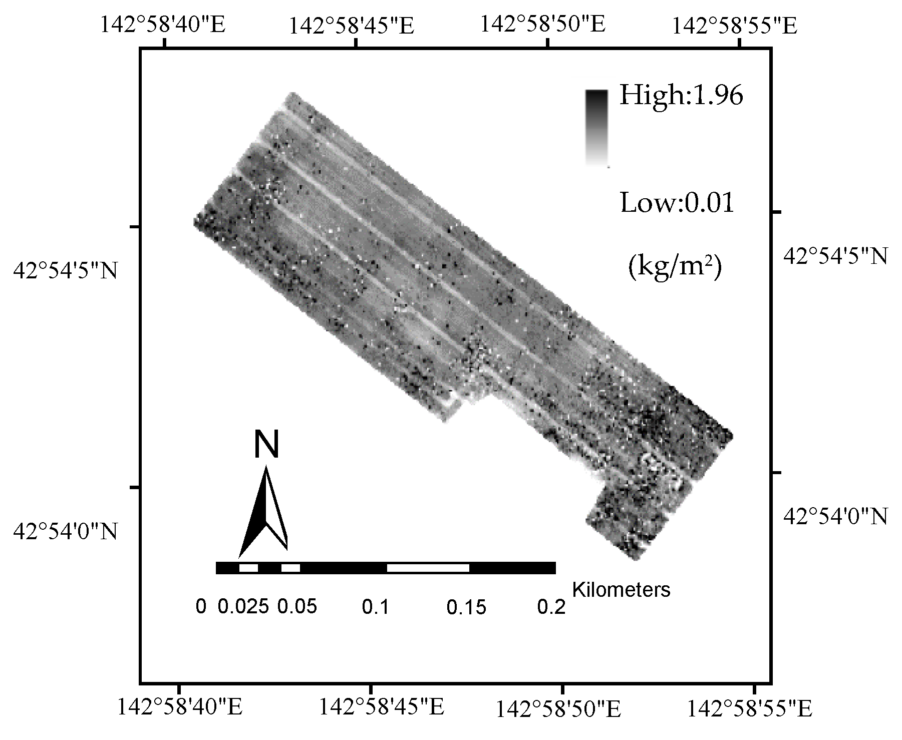
3.3. Mapping of Wheat Yield’s within-Field Spatial Variations

As mentioned in Section 1, it was reported that accumulative CVI values of multi-temporal remote sensing images after flowering stage have good relationship with crop yield. In this paper, we conducted stepwise regression analysis of sampled wheat yield with five different accumulative CVIs extracted from eight orthomosaic images that covered a winter wheat field from heading stage to ripening stage. As described in Section 2 and Section 4, accumulative values of each CVI were obtained by extracting averaged values of pixels that fall within 1-square-meter area around the locations of nine wheat yield samples in each accumulative CVI maps of ExG, NGBDI, GRRI, NGRDI, and VDVI, listed in

Table 4. Accumulative values of each color vegetation index.

Sample ID	VDVI	NGRDI	NGBDI	GRRI	ExG
1	0.71	1.00	0.50	10.40	333.17
2	0.65	1.16	0.29	10.86	264.30
3	0.62	1.04	0.29	10.49	286.08
4	0.64	1.11	0.27	10.70	296.75
5	0.67	1.10	0.33	10.65	301.90
6	0.62	1.12	0.24	10.70	276.56
7	0.62	1.19	0.18	11.00	259.11
8	0.63	1.16	0.25	10.81	244.95
9	0.62	1.19	0.18	10.96	259.36

.

By using stepwise method, a regression analysis was performed in MATLAB R2013a (The MathWorks, Inc., Natick, MA, USA) among the response variable of sampled wheat yield (listed in Table 2) and the predictive variables of accumulative CVI s (listed in Table 4). The result showed that the variable of NGRDI was removed from the stepwise regression model, while the rest variable of CVIs were included to fit the regression model expressed as following, with coefficient of determination as 0.94 and RMSE = 0.02:

Y = −6.19 − 6.78 × X1 + 3.45 × X3 + 0.88 × X4 + 0.003 × X5

(6)

where Y, X1, X3, X4, and X5 denotes estimated wheat yield, accumulative VDVI, NGBDI, GRRI, and ExG, respectively. Subsequently, leave-one-out cross-validation (LOOCV) [27] was also conducted in MATLAB by building nine linear regression models which uses eight set variables of sampled wheat yield and values of CVIs of VDVI, NGBDI, GRRI, and ExG as training data, whilst leaves one set of variables as test data. According to Equation (7) [28], root-mean-square error of prediction (RMSEP) and correlation coefficient r were calculated as 0.06 and 0.69, respectively.

$$\mathrm{RSMEP}=\sqrt{\frac{{{\displaystyle \sum }}_{i=1}^9{\left(y_p-y_m\right)}^2}{9}}$$

(7)

where $y_p$ and $y_m$ denotes predicted value of wheat yield according to each linear regression models by using training data mentioned above and test data of measured grain weight per square meter, respectively. Based on the regression model expressed as Equation (6), wheat yield was calculated by extracting each pixel values of accumulative CVI maps of VDVI, NGBDI, GRRI, and ExG in ENVI software, and map of wheat yield was generated accordingly. Wheat yield’s within-field spatial variations could be observed from the map shown in Figure 10. From wheat yield map we obtained the information that about 25.8% areas in the studied field had grain weight per square meter below 0.5 kg; whilst grain weight per square meter of most areas reached between 0.5–1.5 kg, occupying about 50.4% acreages; and the mean value of grain weight per square meter was calculated as 0.72 kg, which indicated the estimated average yield of the studied field as 7.2 t/ha.

4. Uncertainties, Errors, and Accuracies

The civilian use of UAVs opens up a new way of obtaining field information that is both time and cost efficiently for precision agriculture. Wang et al. [11] successfully differentiated vegetation areas from non-vegetation areas by analyzing color images acquired from a UAV. Rasmussen et al. [14] investigated four different vegetation indices acquired from a color camera and a color-infrared camera by using both a fixed-wing UAV and a rotary-wing UAV, and concluded that vegetation indices based on UAV imagery have the same ability to quantify crop responses with ground-based recordings. However, when UAV imagery was applied into quantitative remote sensing, special attention should be paid to the process of ground truth samplings. In this study, we carefully selected nine grain weight samples to conduct stepwise regression analysis with five color vegetation indices, and cross validation also showed good predicative validity. The small size of the wheat field might also contribute to a certain extent to the significant validity of the regression model, and we cannot guarantee the applicability into other crop field before massive sampling is conducted over several farmlands around a large area. Since the altitude of UAV flight affects image resolution severely, which in turn changes the vegetation index’s value by weakening or strengthening background (soil or crop residues) interferences, appropriate flight altitude should also be taken into consideration when conducting quantitative analysis. Study on vegetation indices also showed that accumulative VDVI + NGBDI + ExG correlated with accumulative NGRDI+GRRI with the correlation coefficient as −0.84, whist accumulative VDVI correlated with sampled grain weight per square meter with the correlation coefficient as 0.85. Therefore, regression analysis using different combination of vegetation indices might also affect the validity of regression model.

5. Conclusions

From multi-temporal UAV orthomosaic images we could visualize the rapid change of wheat growth status through image interpretation and discerned that the canopy greenness of the wheat field of study reached peak condition on 2 July 2015 and the process of yellowing began thereafter. We could also see within-field variation of wheat tiller densities, especially from an early stage of wheat growth from the image taken on 2 June 2015. The occurrence of lodging could also be spotted in orthomosaic images taken on 16 July and 24 July 2015. Therefore, we reached the conclusion that orthomosaic UAV images taken at early stage of wheat growth could be used as prescription of variable-rate fertilizing to avoid, or alleviate, the occurrence of lodging by reducing dozes of fertilizer around over-high tiller density areas. The orthomosaic image taken ahead of harvesting could be used to generate navigation maps that guide either drivers of combine harvesters, or autonomous harvesting vehicles, to adjust operation speed according to the specific lodging situations.

Through stepwise regression analysis of the response variable of sampled grain weight per square meter and the predictive variables of accumulative color vegetation indices, we can conclude that only the variable of normalized green-red difference index was removed from the stepwise regression model due to insignificant p-value, whilst the rest variables of visible-band difference vegetation index (the normalized green-blue difference index, green-red ratio index, and excess green vegetation index) were included to fit the regression model, with coefficient of determination and RMSE as 0.94 and 0.02, respectively. The averaged value of sampled grain weight per square meter was 0.86 kg. The regression model was also validated by using leave-one-out cross validation method, which showed that the root-mean-square error of predication of the regression model was 0.06.

Based on the stepwise regression model, a map of estimated grain weight per square meter (yield map) was generated by extracting each pixel values out of the maps of accumulative vegetation indices. Within-field spatial variations of wheat yield could be observed from the map, which could be seen as the comprehensive presentation of the spatial variations of soil fertility, tiller density, effective water potential, canopy aeration condition, and so on. We also obtained general information of the studied field that about 25.8% areas in the studied field had grain weight per square meter below 0.5 kg, whilst grain weight per square meter of most areas reached between 0.5–1.5 kg, occupying about 50.4% acreages. The mean value of grain weight per square meter was calculated as 0.72 kg, which indicated the estimated average yield of the studied field as 7.2 t/ha.

References

1. Rouse, J.W.; Haas, R.H.; Schell, J.A.; Deering, D.W. Monitoring Vegetation Systems in the Great Plains with ERTS. In Proceedings of the Third ERTS Symposium, NASA, Greenbelt, MD, USA, 10–14 December 1973; pp. 309–317. Available online: https://ntrs.nasa.gov/archive/nasa/casi.ntrs.nasa.gov/19740022614.pdf (accessed on 10 December 2015).
2. Roberto, B.; Paolo, R. On the use of NDVI profiles as a tool for agricultural statistics: The case study of wheat yield estimate and forecast in Emilia Romagna. Remote Sens. Environ. 1993, 45, 311–326. [Google Scholar] [CrossRef]
3. Basnyat, P.; McConkey, B.; Lafond, G.P.; Moulin, A.; Pelcat, Y. Optimal time for remote sensing to relate to crop grain yield on the Canadian prairies. Can. J. Plant Sci. 2004, 84, 97–103. [Google Scholar]
4. David, J.M. Twenty five years of remote sensing in precision agriculture: Key advances and remaining knowledge gaps. Biosyst. Eng. 2013, 114, 358–371. [Google Scholar]
5. Robert, N.C. Determining the prevalence of certain cereal crop diseases by means of aerial photography. Hilgardia 1956, 26, 223–286. [Google Scholar] [CrossRef]
6. Thomas, J.; Trout, L.; Johnson, F.; Jim, G. Remote Sensing of Canopy Cover in Horticultural Crops. Hortscience 2008, 43, 333–337. [Google Scholar]
7. Du, M.M.; Noboru, N. Multi-temporal Monitoring of Wheat Growth through Correlation Analysis of Satellite Images, Unmanned Aerial Vehicle Images with Ground Variable. In Proceedings of the 5th IFAC Conference on Sensing, Control and Automation Technologies for Agriculture AGRICONTROL, Seattle, WA, USA, 14–17 August 2016.
8. Eisenbeiss, H. A Mini Unmanned Aerial Vehicle (UAV): System Overview and Image Acquisition. In Image Acquisition. In Proceedings of the International Workshop on Processing and Visualization Using High-Resolution Imagery, Pitsanulok, Thailand, 18–20 November 2004.
9. The Third National Agricultural Census Using UAV Remote Sensing. Available online: http://www.uavwrj.com/gne/427.html (accessed on 25 October 2016).
10. James, B.C.; Randolph, H.W. Introduction to Remote Sensing, 5th ed.; The Guilford Press: New York, NY, USA, 2011; pp. 72–102. [Google Scholar]
11. Wang, X.Q.; Wang, M.M.; Wang, S.Q.; Wu, Y.D. Extraction of vegetation information from visible unmanned aerial vehicle images. Trans. Chin. Soc. Agric. Eng. 2015, 31, 152–159. [Google Scholar]
12. Feng, J.L.; Liu, K.; Zhu, Y.H.; Li, Y.; Liu, L.; Meng, L. Application of unmanned aerial vehicles to mangrove resources monitoring. Trop. Geogr. 2015, 35, 35–42. [Google Scholar]
13. Raymond Hunt, E., Jr.; Dean Hively, W.; Fujikawa, S.J.; McCarty, G.W. Acquisition of NIR-Green-Blue Digital Photographs from Unmanned Aircraft for Crop Monitoring. Remote Sens. 2010, 2, 290–305. [Google Scholar] [CrossRef]
14. Rasmussen, J.; Ntakos, G.; Nielsen, J.; Svensgaard, J.; Poulsen, R.N.; Christensen, S. Are vegetation indices derived from consumer-grade cameras mounted on UAVs sufficiently reliable for assessing experimental plots? Eur. J. Agron. 2016, 74, 75–92. [Google Scholar] [CrossRef]
15. Torres-Sánchez, J.; Peña, J.M.; de Castro, A.I.; López-Granados, F. Multi-temporal mapping of the vegetation fraction in early-season wheat fields using images from UAV. Comput. Electron. Agric. 2014, 103, 104–113. [Google Scholar] [CrossRef]
16. Woebbecke, D.M.; Meyer, G.E.; Von Bargen, K.; Mortensen, D.A. Color Indices for Weed Identification under Various Soil, Residue and Lighting Conditions. Trans. ASAE 1995, 38, 259–269. [Google Scholar] [CrossRef]
17. Cui, R.X.; Liu, Y.D.; Fu, J.D. Estimation of winter wheat biomass using visible spectral and BP based artificial neural networks. Spectrosc. Spectr. Anal. 2015, 35, 2596–2601. [Google Scholar]
18. Global Wheat Production from 1990/1991 to 2016/2017 (in Million Metric Tons). Available online: https://www.statista.com/statistics/267268/production-of-wheat-worldwide-since-1990/ (accessed on 20 October 2016).
19. Wu, Q.; Wang, C.; Fang, J.J.; Ji, J.W. Field monitoring of wheat seedling stage with hyperspectral imaging. Int. J. Agric. Biol. Eng. 2016, 9, 143–148. [Google Scholar]
20. Zhang, F.; Wu, B.; Luo, Z. Winter wheat yield predicting for America using remote sensing data. J. Remote Sens. 2004, 8, 611–617. [Google Scholar]
21. Ministry of Agriculture, Forestry, and Fisheries. Available online: http://www.maff.go.jp/ (accessed on 10 November 2016).
22. Trimble SPS855 GNSS Modular Receiver. Available online: http://construction.trimble.com/sites/default/files/literature-files/2016-07/SPS855-Data-Sheet-EN.pdf (accessed on 12 November 2015).
23. Weather Time-Memuro. Available online: https://weather.time-j.net/Stations/JP/memuro (accessed on 2 December 2016).
24. Júnior, O.A.D.C.; Guimarães, R.F.; Silva, N.C.; Gillespie, A.R.; Gomes, R.A.T.; Silva, C.R.; De Carvalho, A.P.F. Radiometric normalization of temporal images combining automatic detection of pseudo-invariant features from the distance and similarity spectral measures, density scatterplot analysis, and robust regression. Remote Sens. 2013, 5, 2763–2794. [Google Scholar] [CrossRef]
25. Torres-Sanchez, J.; Lopez-Granados, F.; De Castro, A.; Pena-Barragan, J.M. Configuration and Specifications of an Unmanned Aerial Vehicle (UAV) for Early Site Specific Weed Management. PLoS ONE 2013, 8, e58210. [Google Scholar] [CrossRef]
26. Gamon, J.A.; Surfus, J.S. Assessing leaf pigment content and activity with a reflectometer. New Phytol. 2013, 143, 105–117. [Google Scholar] [CrossRef]
27. Michael, K.; Dana, R. Algorithmic stability and sanity-check bounds for leave-one-out cross-validation. Neural Comput. 1999, 11, 1427–1453. [Google Scholar]
28. Feng, Q.S.; Gao, X.H. Application of Excel in the Experiment Teaching of Leave-One-Out Cross Validation. Exp. Sci. Technol. 2015, 13, 49–51. [Google Scholar]
Figure 1. Proposed method of estimating wheat yield by using unmanned aerial vehicle (UAV) images.
Remotesensing 09 00289 g001
Figure 2. Field site of the test farmland in Memuro, Hokkaido, Japan.
Remotesensing 09 00289 g002
Figure 3. Winter wheat field of study was shown in black rectangle (ground control points were marked as black dots).
Remotesensing 09 00289 g003
Figure 4. Quadrotor used as platform of UAV-camera system (left image), and UAV’s flight path (right image).
Remotesensing 09 00289 g004
Figure 5. Spatial distribution of UAV images’ pseudo-invariant features (PIFs).
Remotesensing 09 00289 g005
Figure 6. Wheat samples’ spatial distribution.
Remotesensing 09 00289 g006
Figure 7. CVI maps on 2 June 2015 and accumulative ExG map of the test wheat field.
Remotesensing 09 00289 g007
Figure 8. Orthomosaic images of the test wheat field from heading stage to harvesting.
Remotesensing 09 00289 g008
Figure 9. Close-shot photograph of the lodging spot in test wheat field, taken on 16 July 2015.
Remotesensing 09 00289 g009
Figure 10. Map of wheat yield (expressed as grain weight per square meter).
Remotesensing 09 00289 g010