A Hierarchical Maritime Target Detection Method for Optical Remote Sensing Imagery

Abstract

Maritime target detection from optical remote sensing images plays an important role in related military and civil applications and its weakness lies in its compromised performance under complex uncertain conditions. In this paper, a novel hierarchical ship detection method is proposed to overcome this issue. In the ship detection stage, based on Entropy information, we construct a combined saliency model with self-adaptive weights to prescreen ship candidates from across the entire maritime domain. To characterize ship targets and further reduce the false alarms, we introduce a novel and practical descriptor based on gradient features, and this descriptor is robust against clutter introduced by heavy clouds, islands, ship wakes as well as variation in target size. Furthermore, the proposed method is effective for not only color images but also gray images. The experimental results obtained using real optical remote sensing images have demonstrated that the locations and the number of ships can be determined accurately and that the false alarm rate is greatly decreased. A comprehensive comparison is performed between the proposed method and the state-of-the-art methods, which shows that the proposed method achieves higher accuracy and outperforms all the competing methods. Furthermore, the proposed method is robust under various backgrounds of maritime images and has great potential for providing more accurate target detection in engineering applications.

1. Introduction

Maritime ship target detection and recognition by Unmanned Airborne Vehicles (UAVs) and satellites is an active research field and plays a crucial role in a spectrum of related military and civil applications, such as naval defense and security, traffic surveillance, maritime rescue, protection against illegal fisheries, anti-smuggling efforts, oil discharge control, and sea pollution monitoring, for which automatic ship detection and ship recognition are important to the protection of coastlines and exploration of the vast and rich marine resources.

Ship targets are mainly divided into three categories based on the types of images: synthetic aperture radar (SAR) images, infrared (IR) images and visible images [1]. SAR images have been the most widely studied since they can be obtained during both day and night regardless of weather conditions. Many approaches for SAR images have been proposed, such as constant false-alarm rate (CFAR) methods based on all kinds of distributions [2,3,4], the fractal detection algorithm [5] and wavelet transform [6]. However, accurate detection of targets with these methods remains challenging. For example, only target points can be obtained in SAR-based images, which lack color and texture features. The revisit cycle is relatively long, and wooden boats may be invisible to radar. Recently, SAR altimetry [7,8] has shown the potential to resolve non-water targets as well as electromagnetic features connected with the sea state, with the possibility of providing global ship traffic statistics with a relatively short revisit time and free data. It does not provide images, but can be considered as a complement to the ship detection based on SAR techniques. IR images are often applied to reveal the locations of hidden targets and enhance vision under weak light conditions. However, their use is limited by poor Signal Noise Ratio (SNR) and changeable gray levels, and a number of challenges remain in the current methods, including target segmentation [9,10,11] and contour extraction [12]. Compared with the previous two categories of images, images in the visible bands are more intuitive, easier to understand, and have a higher resolution, more detailed ship information and more obvious geometric structures. In this study, we focus on detecting ships in the visible bands of optical remote sensing images. However, there are still plenty of difficulties in this field. For instance, a ship’s appearance may vary greatly due to uneven illumination, the viewing geometry and the variability of ship sizes. In addition, the sea surface is complex due to interference from clouds and haze, sea clutters, ship wakes, small islands, and coastlines, among others, which may be falsely detected as ships, leading to false alarms and increasing processing time. Therefore, determining how to accurately and quickly detect ship targets in the marine background is an urgent problem.

Aiming at these problems addressed above, we have made an in-depth investigation into existing approaches. Some detection methods have been devised for ship wakes [13,14,15]. However, ship wakes exhibit relatively large variation, which is related to the navigation speeds. Sometimes, ship wakes may not even exist. Therefore, our detection method, alternatively, focuses on ship targets themselves rather than ship wakes. The current approaches for ship targets detection in the literature can be mainly summarized as follows. Some approaches can be roughly considered as gray statistics and threshold segmentation. For instance, Burgess [16] proposed a method that includes masking, filtering and shape analysis techniques to detect ships in optical images. The method in [17] put forward a complete set of sea surface ship detection processing chains. There, the target region is extracted by using statistical and morphological filtering, and false alarms are reduced through wavelet analysis and the Radon transform. Proia [18] estimated the Gaussian distribution of the sea background density function and applied Bayesian decision theory to discriminate small ships. Yang [19] employed a linear function combining pixel and region features to select ship candidates after sea surface analysis. Xu [20] proposed a method of multiscale contour extraction using level sets. These methods are suitable for sea conditions with uniform texture and low gray level. However, they are sensitive to complex sea backgrounds, such as heavy clouds, small islands, uneven illumination, and sea clutters. Besides, the black and white polarity of ships easily causes false alarms. If the intensity level of a ship is similar to that of its surroundings, it is difficult to extract the ship. Other type of ship detection methods rely on supervised classification. Great attention has been paid to the different kinds of features as well as various classifiers. Corbane [21] extracted feature sets after segmentation. The detection was accomplished with a genetic algorithm and neural networks. The support vector machine (SVM) classifier based on shape and texture features was used in [22] to reduce the false alarms. Xia [23] came up with a ship extraction algorithm that fused several geometrical features by using the dynamic fusion model and detected ships using SVM. Classification algorithms using color, texture and local shape feature for ship detection were introduced in [24,25]. Each of these methods essentially includes an improvement in either preprocessing or classification, to achieve better performance. However, these methods require the production of a large number of templates and rely on prior knowledge. Furthermore, they face difficulties in practical applications. In addition to the above methods, there are other categories of detection methods that can resist interference from complex backgrounds and detect objects with fuzzy appearances effectively. Duan [26] explored several techniques using a contour matching approach and an improved optimization algorithm. Sun [27] presented an automatic target detection framework by using a spatial sparse-coding bag-of-words model. Cheng [28,29,30] developed a practical and rotation-invariant framework for multi-class geospatial object detection and classification based on a collection of part detectors. Han [31] proposed a method of multi-class geospatial target detection by the integration of visual saliency modeling and the discriminative learning of sparse coding. Naoto [32] integrated sparse representations for local-feature detection into generalized-Hough-transform ship detection. Wang [33] proposed a framework for multi-class object detection based on the discriminative sparse representation. The performances of these methods are satisfying in terms of detection and recognition. However, their computational complexities are greatly increased. The computation time increases exponentially when dealing with complex and drastically varying conditions. Such approaches are obviously time-consuming and unsuitable for real-time processing. Even worse, some small targets may not be captured.

Recently, it has become well known that the visual saliency model can quickly access to information associated with current scene and task, even for a highly cluttered scene. This advantage has made it a hot spot in ship detection. Visual saliency models can be mainly divided into two types: the goal-driven top-down models and the data-driven bottom-up models. A top-down model is related to specific tasks and goals, which use cognitive factors such as pre-knowledge, context information, expectations, and motivations to perform a visual search. Bi [34] proposed a multiscale and hierarchical model based on contextual information to detect ships. Zhu [35] presented a top-down model in which the coding-based classification framework and spatial context information is exploited for goal-driven visual detection. However, the existing top-down models usually carry a high computational cost and are without a generic model. As another essential source of bottom-up cues, most saliency detection models are based on this mechanism. They can be divided into spatial domain models and frequency domain models. The spatial domain models mainly include the ITTI model (devised by Itti et al.) [36], AIM model (Attention based on Information Maximization) [37], GBVS model (Graph-Based Visual Saliency) [38], CA model (Context Aware, also known as the Goferman model) [39], LC model (Linear Contrast) [40], HC model (Histogram Contrast) [41], and FT model (Frequency-Tuned Saliency) [42]. The targets are obtained by integrating multiple features. However, these models are relatively time-consuming and are easily influenced by sea conditions, and their performance on background suppression is limited. Compared with spatial domain models, frequency domain models have more advantages in terms of computation speed and background suppression. Hou [43] proposed the SR detection model (Spectral Residual), which can process a single channel grayscale image, where saliency detection is firstly considered as a frequency domain problem. Then, the PQFT model (Phase Quaternion Fourier Transform) [44] and the PBFT model (Phase Spectrum of Biquaternion Fourier Transform) [45] were proposed to process multi-channel features of color images. These models have good performances in target edge detection, whereas low integrity in targets, especially for large targets. Li [46] presented the HFT model (Hypercomplex Frequency Domain Transform), which can detect the target and maintain its integrity. However, the background suppression ability is relatively poor, especially for targets that are too close to each other. Lin [47] proposed an image-block-based approach, in which saliency detection is carried out in each block, and the saliency maps are subsequently combined. However, the false alarm rate of this approach is heavily influenced by the sea clutter and would greatly increase in the presence of thick clouds and small islands. Corbane [17] combined the statistical methods and a morphology filter to mask out thin clouds. However, thick clouds still cannot be removed effectively.

Therefore, despite the numerous approaches that have been developed, we are still far from solving the problems in ship detection from optical remote sensing images. The desired detector should not only extract ships but also remove false alarms. Focused on these problems, a hierarchical ship detection scheme is proposed in this paper. Two major ideas including prescreening and discrimination are composed and emphasized. For the former, a visual saliency model is used. We have improved the existing models and further constructed a practical combined saliency model, which integrates multi-frequency information using self-adaptive weights based on Entropy information. It is effective in identifying both large and small ships and suppressing interference from complex backgrounds. In addition to achieving higher accuracy, our model is not sensitive to parameter settings and can be automatically executed. After extracting candidates, some pseudo-targets are also obtained in addition to real ships. Therefore, a novel ship descriptor is designed for confirming whether the targets are real ships, where gradient features are used and some efficient rules are applied. This step is vital for reducing false alarms. However, in some existing methods, it is simplified or even not considered [20,45]. Our method is different from the other methods proposed in the literature, and has achieved necessary improvements in saliency detection, image segmentation, and feature extraction for discriminating targets. Compared with the previous works, our approach can achieve better performance in terms of detection accuracy.

The rest of this paper is organized as follows. In Section 2, the framework of visual saliency detection is given and our ship candidate detection model is introduced. In Section 3, the gradient-feature descriptor is designed to discriminate real ships. In Section 4, the execution of the proposed method is illustrated. Also provided in this section are a quantitative comparison and an evaluation. Finally, the conclusion and possible extensions are discussed in Section 5.

2. Ship Candidates Extraction Based on Visual Saliency

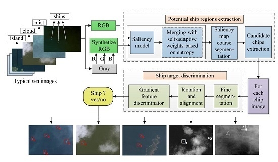
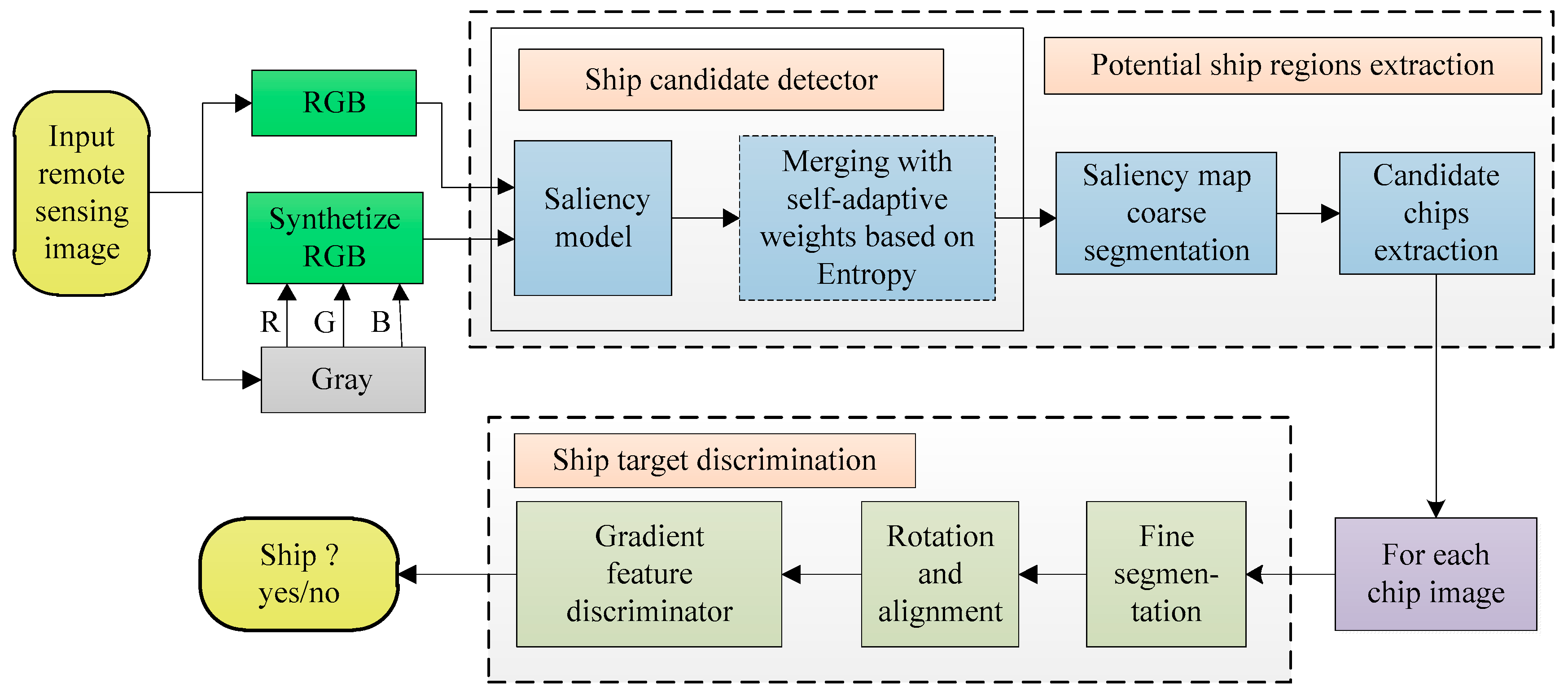
2.1. Overall Framework

In this paper, our study aims at detecting ships in open oceans. The interference from the land area can be eliminated using prior geographic information, for instance, a GIS database. The overview of our detection algorithm is given in Figure 1, which covers the whole process from coarse to fine detection. Images in the visible bands of optical remote sensing data are used to validate the detection accuracy and robustness of our method. Note that if the input image is a color image, it can be calculated directly. Otherwise, a conversion into a synthetic color image is needed. In the prescreening stage, the potential ship targets are extracted using the combined saliency model based on Entropy information. Then, the residual false alarms are further removed by the descriptor in the discrimination stage.

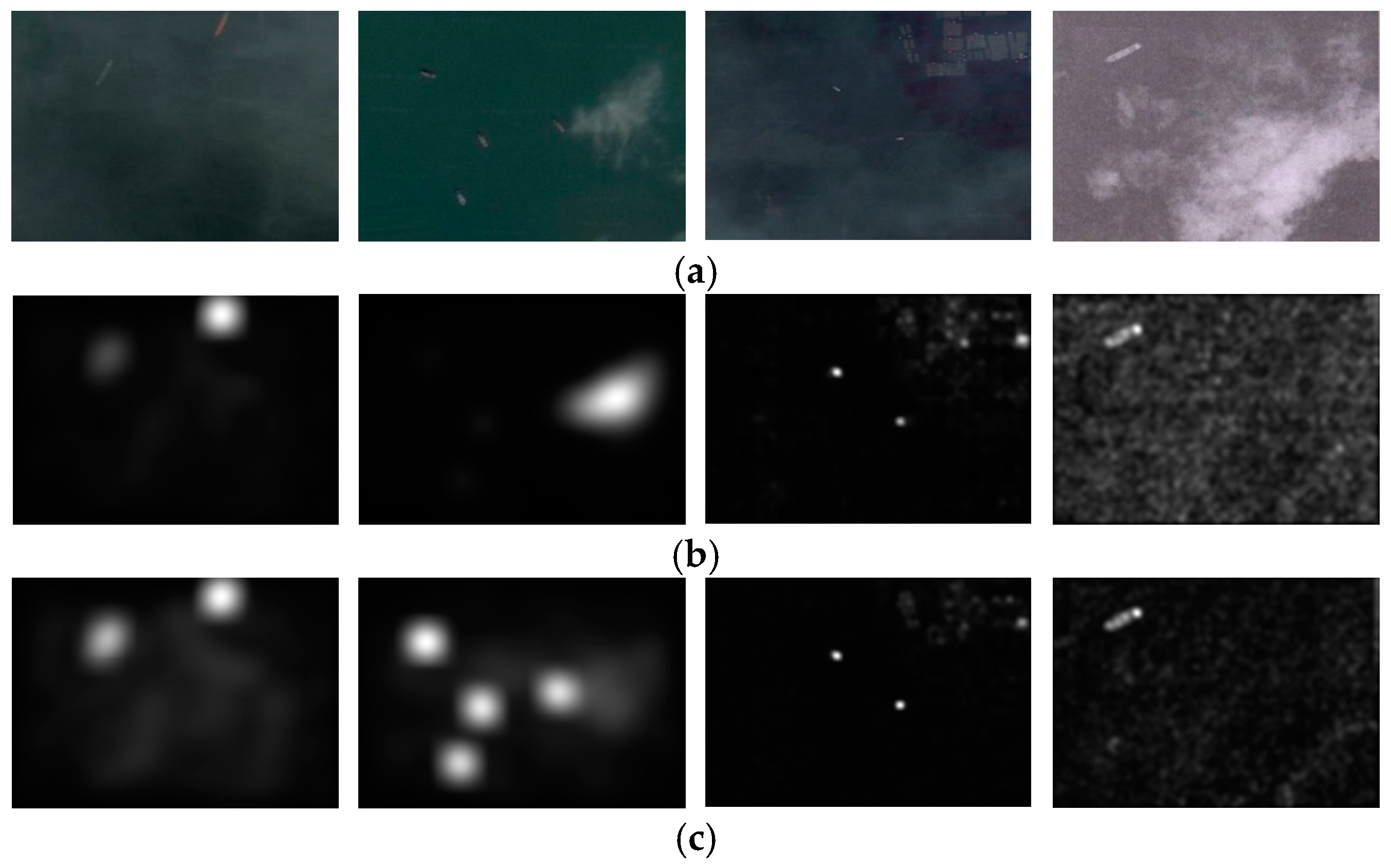
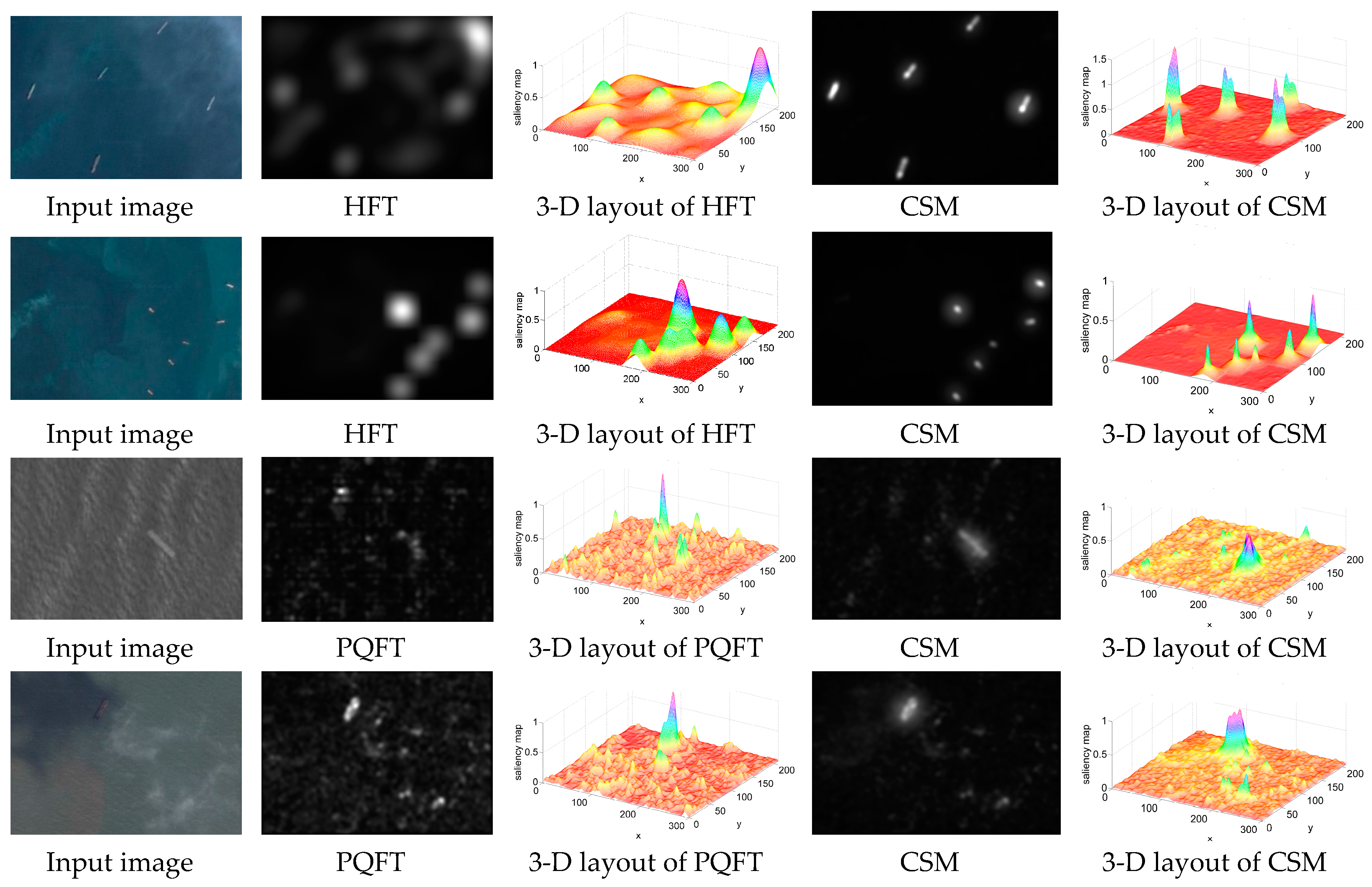
2.2. Saliency Detection Model

In the first stage, as described in Figure 2, the saliency detection model based on the frequency domain is used for quickly finding and extracting candidate target regions. The ship candidates can be obtained by coarse segmentation and marking. The goal of this stage is to detect ship targets as accurately as possible and detect false alarms as rarely as possible.

The following sections describe the major steps of our saliency model in detail. Visual saliency has been widely used to highlight valuable targets while suppressing the background. For the HFT model, the targets in a color image can be extracted with the hypercomplex form. Brightness I, red-green C_RG and blue-yellow C_BY are used to construct the color features. Since the input image is static, the motion feature is not considered and its value is set to zero. Given a color image f(x,y), it can be represented by a quaternion matrix [46] as follows:

$$q(x,y)=0.25\times C_{RG}{u}_1+0.25\times C_{BY}{u}_2+0.5\times I{u}_3$$

(1)

where x and y denote the pixel co-ordinates in the spatial domain. u₁, u₂ and u₃ are unit pure quaternions obeying the following rules: u₁² = u₂² = u₃² = −1, u₁⊥u₂, u₂⊥u₃, u₃⊥u₁, and u₁ × u₂ = u₃. The feature sequence does not affect the results of the calculation. An image represented by quaternions is shown in Figure 3.

When the ship targets are directly detected using the HFT model, the sea background interference suppression ability is not strong. Some very weak and dim targets may be missed. In addition, when multiple targets are too close to each other, the model’s distinguishing ability is weak. The PQFT model has also been used for extracting the multi-channel features of a color image for construction of a quaternion matrix and detection. However, the integrity of the target region is poor with the PQFT model, especially for large targets. In addition, it may have inferior performance in some cases including heavy sea clutter and complex textures. Motivated by these shortcomings, we propose an effective saliency detection model and set the following requirements:

• Include complete salient objects.
• Uniformly highlight the entire target regions.
• Disregard high frequencies introduced by clouds, islands, ship wakes and sea clutters.
• Efficiently output the saliency maps with full resolution.

To meet these requirements, we improve the HFT model and modify it using the improved PQFT model with self-adaptive weights. More details are described hereinafter. We improve the HFT model in terms of color, frequency domain transform and scale selection. We use the CIE Lab color space in place of RGB color features in this study. CIE Lab color space is a color-opponent space with dimensions L for lightness and a and b for the color-opponent dimensions. It includes all perceivable colors, which means that its gamut exceeds those of the RGB color models. When a spatial discrete color image is input, it is separated into three-channel images. L, a, and b are the three-channel color features of the input image in the CIE Lab color space. L_m, a_m, and b_m are the arithmetic mean pixel values of L, a, and b over the entire image. The difference between the value at each pixel location of each channel and the average value of all pixels of the image in the corresponding channel is calculated as follows:

$$L_d(x,y)=(L(x,y)-L_m)$$

(2)

$$a_d(x,y)=(a(x,y)-a_m)$$

(3)

$$b_d(x,y)=(b(x,y)-b_m)$$

(4)

Then, the value of each pixel in an image is represented as a quaternion as follows:

$$q(x,y)=L_d(x,y)u_1+a_d(x,y)u_2+b_d(x,y)u_3$$

(5)

The quaternion function representation of the image will be transformed into the frequency domain. We use the Discrete Cosine Transform (DCT) instead of the Discrete Fourier Transform. The DCT is similar to the DFT, but uses only real numbers, which are equivalent to the DFT of roughly twice the length, and operates on real data with even symmetry. In addition to its orthogonal structure, the DCT has a strong energy compaction property, and most of the signal information tends to be concentrated in a few low-frequency components of the DCT [48]. After the transform, a Spectrum Scale-Space is described for handling amplitude spectra at different scales, which is given by:

$$Q[u,v]=DCT(q(x,y))$$

(6)

$$\mathrm{A}(u,v)=\left|Q[u,v]\right|$$

(7)

$$G(u,v;k)=\frac{1}{2\pi \cdot 2^{2k-2}}{e}^{-(u^2+v^2)/(2^{2k-3})}$$

(8)

$$\Lambda (u,v;k)=(G(.,.;k)\times \mathrm{A})(u,v)$$

(9)

where u and v denote the pixel co-ordinates in the frequency domain; DCT(·) denotes the Discrete Cosine Transform and A(·) represents the amplitude spectra. G(·) denotes a series of Gaussian kernels. k is the scale parameter, k = 1, 2, 3. Λ(·) is a family of derived signals defined by the convolution of A(·) with G(·). * denotes the convolution operator.

The optimal one (S’(x,y)) from a series of saliency maps S_k is obtained based on an Entropy criterion. Through Gaussian filtering, the saliency map S₁(x,y) of the improved HFT is expressed by:

$$S_1\left(x,y\right)=g\times {\left(S^{\prime }\left(x,y\right)\right)}^2$$

(10)

where g is a two-dimensional low-pass Gaussian filter.

2.3. Saliency Map Modification Based on Entropy Information

After improving the HFT model, dim targets are enhanced and missed targets are possibly highlighted. Furthermore, if the distance between targets is too small, the aggregation phenomenon may occur. The number of targets cannot be confirmed accurately. Our solution to this issue is to modify the model using an improved PQFT model.

A similar procedure to the one stated above is applied. The Lab color features are used in place of RGB features. We use the DCT instead of the DFT. Different from the original PQFT model, which only uses the phase information, the amplitude information A(·) is also used, and its logarithm value is calculated from Equation (11) and used in place of A(·).

$$AL=\log (A)=\log (\left|Q[u,v]\right|)$$

(11)

Then, the saliency map S₂(x,y) based on the improved PQFT model is obtained.

Some detection results before and after improvements are displayed in Figure 4. The first two columns compare the improved HFT with the original HFT models. We find that the dim targets may be missed using the original HFT model directly. After the improvement, the ship regions are more highlighted. The latter two columns compare the improved PQFT with the original PQFT models. It is noted that the suppression of background interference is more effective after improvement.

Although the results after improving are promising, there are some possible problems to be resolved such as the aggregation phenomenon in the HFT model and the discontinuities in the PQFT model. These problems may still occur after the improvement and further improvements are needed, as follows.

We merge the saliency maps S₁(x,y) and S₂(x,y) automatically based on the following formula and the result takes the advantages of the two models. Before merging, the saliency maps from the two models are scaled to [0, 1]. The final map S(x,y) is calculated as follows:

$$S\left(x,y\right)=w_1\times S_1\left(x,y\right)+w_2\times S_2\left(x,y\right)$$

(12)

where w₁ and w₂ are self-adaptive weights. In order to process saliency information automatically, we use the Entropy information to determine the appropriate weights.

For the desired saliency map, the target region should be highlighted and the background clutter should be suppressed. Thus, the saliency map can be considered as a probability map and the histogram of the map should cluster around certain values, which will yield a corresponding Entropy value. When the value reaches minimum, the optimal saliency map would be found. Inspired by this fact, the weight is given by:

$$w_k={\left(H\left(S_k\left(x,y\right)\right)\right)}^{-1}$$

(13)

where k is the subscript, k = 1, 2. w₁ and w₂ are weights. S₁(x,y) and S₂(x,y) represent the improved HFT and PQFT saliency maps, respectively. H(·) is the function for calculating the Entropy of the saliency map, defined as:

$$H(p)=-{\displaystyle {\sum }_i^n{p}_{i}lo{g}_2{p}_i}$$

(14)

where p_i contains the histogram counts returned from an image. The index i is the grayscale, i = 0, 1, 2, …, 255. The saliency detection results of the original HFT model, the original PQFT model, and our combined saliency map (CSM) model are compared, as shown in Figure 5.

As shown in Figure 5, the CSM model generates clearer contour and more uniformly highlighted salient regions as compared to the original HFT and PQFT models. The first two rows compare the CSM with the original HFT models. The corresponding energy distribution maps before and after modification are given. Note that the aggregation phenomenon generated in the HFT model is weakened by this improvement. The ability to distinguish different targets in the CSM model is enhanced. The last two rows are the comparisons between the CSM and the PQFT models. We note that the sea clutter in the maps is obvious and strong before improvement. The background interference around the ships is well suppressed in the CSM model. Most of the thin clouds, mist and sea clutter are removed, and the ship targets are effectively extracted. In the third row, the target region is not complete and not uniform using PQFT. While this problem has been resolved in the CSM model. In addition, the CSM model runs automatically without requiring parameters adjustment.

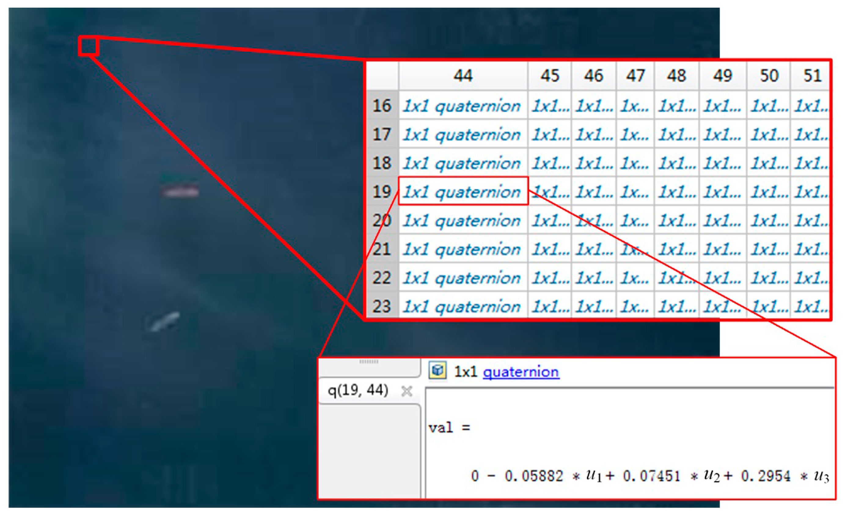
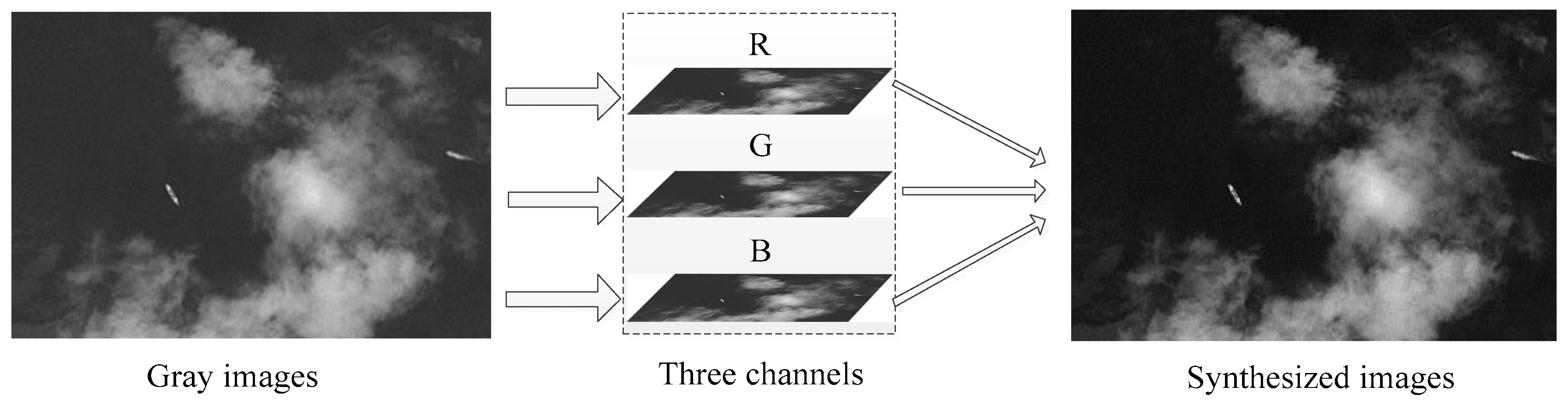
2.4. Gray Image Processing

In addition to color images, some images may be gray in certain cases. To address these cases, a pre-processing step is needed, as shown in Figure 6. A gray image is viewed as a single-channel special case of a three-channel color image. First, a three-channel image space is constructed and initialized to zero. The pixel values of the gray image are assigned to this space, and this step is repeated three times. Then, a synthesized RGB image is obtained, and the following processing is similar to that for color images.

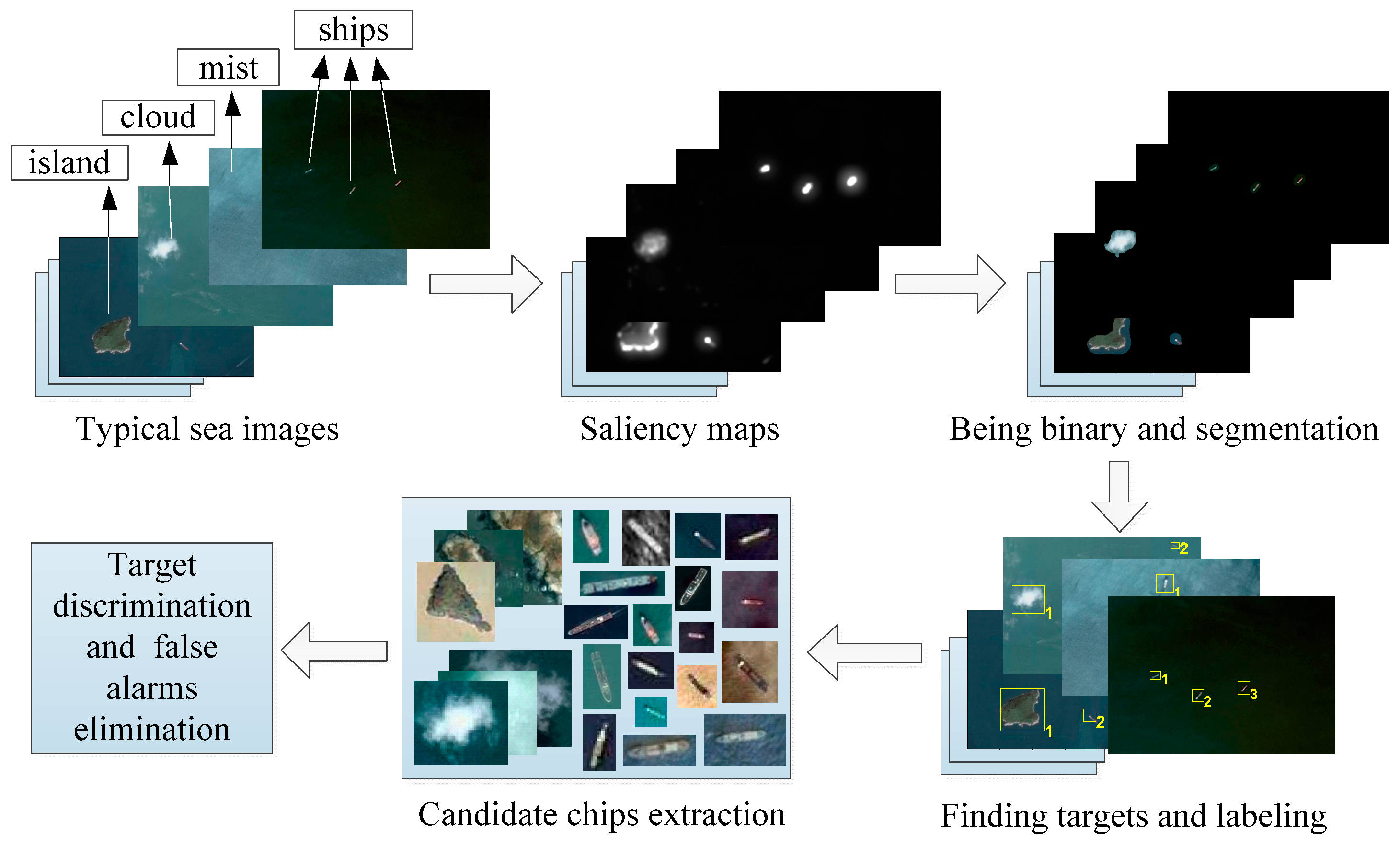
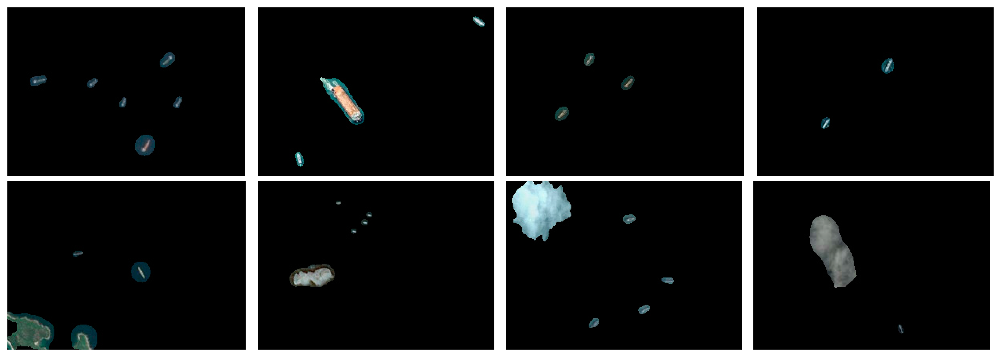
2.5. Target Candidate Extraction

To extract the candidates, an adaptive coarse segmentation based on the Otsu method is performed. The Otsu method [49] is based on a single dimension gray histogram of the image and can automatically maximize the between-class variance of the foreground and back-ground in the histogram. S(x,y) is binarized by the threshold determined with the Otsu method. All pixels higher than the threshold are defined as targets and the rest are considered as the background. After obtaining the corresponding binary images, we multiply the binary images with the original remote sensing images, and the results are shown in Figure 7. Based on the binary maps, we define the connected regions covered by the bounding rectangle as candidates. Some target chips can be obtained in this step. To ensure the integrity of the targets, we extend the size of each chip by 10 pixels along each dimension.

3. Ship Discrimination

After extracting ship candidates, some pseudo-targets, for example, the masks of islands and clouds, may be included. To further reduce these false alarms, other techniques are needed to effectively remove the interference according to the characteristics of ships and non-ship targets. The shape feature of a ship is more regular since a ship appears as a long symmetrical strip, whereas the shapes of the pseudo-targets detected are irregular. Inspired by this fact, a novel descriptor is designed to identify real ships based on gradient features. Before the identification, the target chip must be segmented finely, and the major axis of the ship target must be made symmetrical.

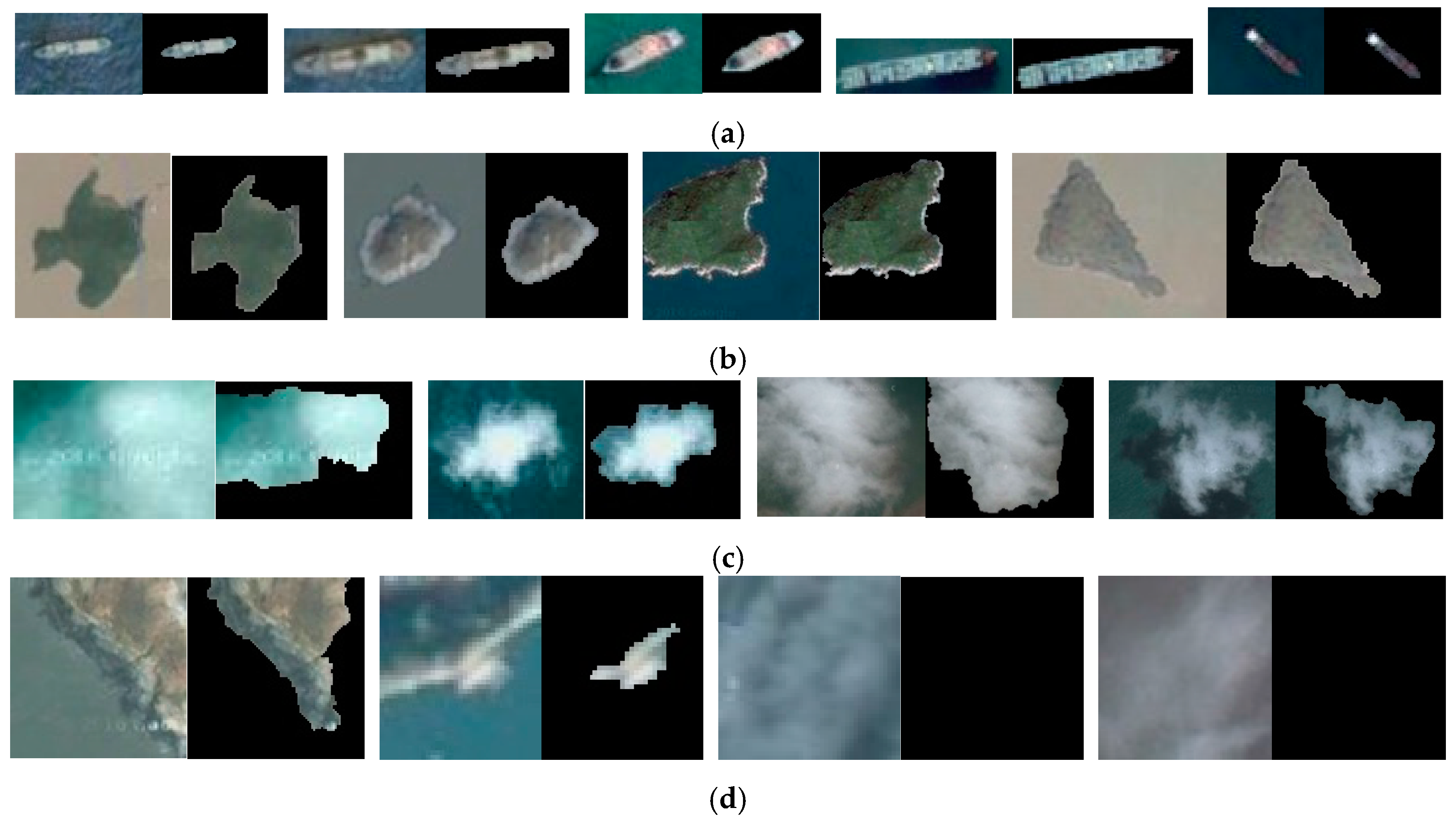
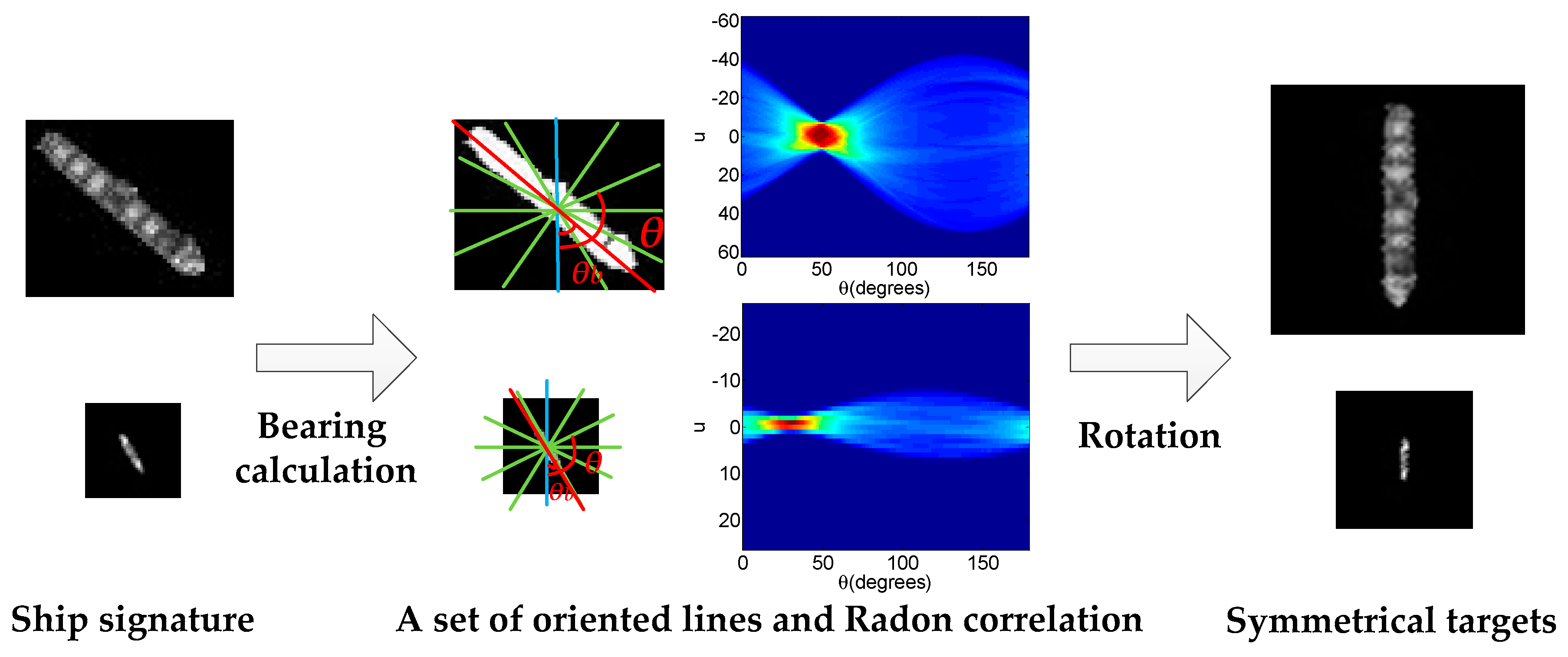
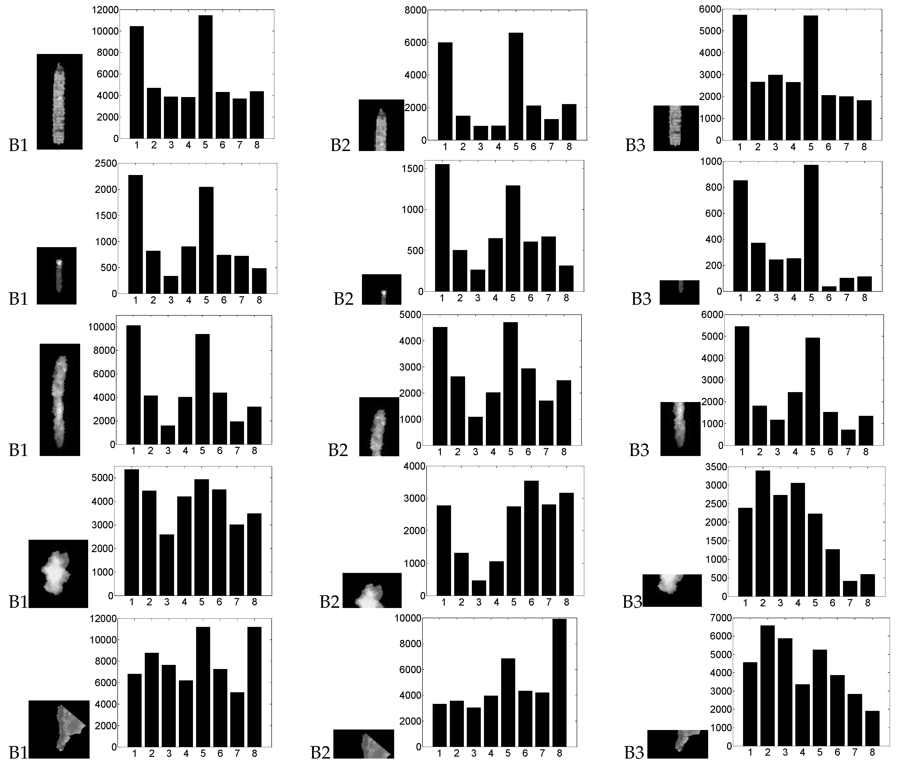
3.1. Fine Segmentation and Symmetry

Currently, the availability of high-resolution images has allowed for more accurate detection of the outline of the ships’ hull. Ship targets have become relatively large targets, unlike the point-like targets in the low-resolution images. Different from the method in [50], we propose an effective segmentation method based on the GrabCut algorithm [51], which is improved based on the GraphCut algorithm. The GrabCut algorithm is an iterative segmentation algorithm based on graph theory. It is widely used in the extraction of foreground objects from a complex environment. The GrabCut creates Gaussian Mixture Models (GMMs) for the background and foreground separately, and adopts an iterative procedure that alternates between parameter learning and segmentation estimation until it converges. A few improvements are made, and the chips are directly addressed instead of segmenting the entire image. The ranges of (4, col-4) and (4, row-4) of the chip are defined as the foreground to be segmented automatically. “col” and “row” are the column and row numbers of the chip. The rest of the chip is the background. The candidate contains only a single target and a small portion of the surrounding area. In general, the number of iterations is set to two. If the sea background is complex or the chip is larger than 60 × 60 pixels, the number of iterations can be set to three. The fine segmentation results are shown in Figure 8. To facilitate the layout, the sizes of the chips are adjusted.

If the chip contains a ship target, the fine segmentation of ships will be obtained, as shown in Figure 8a. The ship candidates are regular in general. In the presence of islands or strong reflection or thick clouds, segmentation results of irregular shape will be obtained, as shown in Figure 8b,c. They are irregular in general. If the background is for the most part evenly distributed, the difference between the target and the background is small. The brightness value of the foreground is zero or close to zero after segmentation as shown in Figure 8d. If the target area in a chip is smaller than 10 pixels, the chip is abandoned. If the target area is oversized, i.e., larger than 3000 pixels, the chip is also rejected.

To obtain a rotation-invariant feature, the target should be symmetrical around the ship principal axis in the vertical direction by rotation and symmetry. Radon transform [52] is used to carry out this task and estimate the ship target heading, which is the projection of the image intensity along a radial line oriented at a specific angle. For a spatial discrete image f(x,y), the general Radon transform is defined as:

$$R\left(\theta ,u\right)={\displaystyle {\int }_{D}f}\left(x,y\right)\delta \left(u-x\cos \theta -y\sin \theta \right)dxdy$$

(15)

where θ represents the angle between the oriented line and the y-axis, and u is the length of the normal from the origin point to the oriented line. The oriented line can be considered as u = xcosθ + ysinθ. D denotes the whole x–y image plane. δ is the Dirac delta-function:

$$\delta (t)=\{\begin{array}{ll}+\infty & t=0\\ 0& t\ne 0\end{array}$$

(16)

where t is a real parameter. The integral of the δ function over the parameter from −∞ to +∞ is equal to one. After Radon transform, the lines in the original image are mapped onto bright and dark spots in Radon space (u,θ). The issue of calculating the ship heading is converted to finding a peak in the Radon transform. The confident heading of the target is equal to θ_b value and u(θ_b) is close to zero, which corresponds to the brightest spot in the map of Radon Transform. Then, we align the target axis to the vertical direction by clockwise rotation of θ_b. The rotation invariance of the gradient distribution is fulfilled. Detailed illustrations are shown in Figure 9.

3.2. Gradient Features

In general, a powerful descriptor identifying the ship target is critical for the final discrimination, which should meet the requirement that it is applicable to ships with different sizes and strong wakes first. As known, a ship always has a large length-to-width ratio, similar to a very elongated ellipse. The gradients of the two ship sides are symmetrical and generally have high magnitudes in their perpendicular directions. Moreover, ship wakes have linear textures. Inspired by these facts, a novel descriptor based on gradient features is designed, which is improved based on the histogram of oriented gradients (HOG) feature. The HOG feature [53] can be used to effectively detect targets in computer vision and image processing. The HOG feature is based on the well-normalized local histograms of image gradient orientations in a dense grid, and it essentially describes the local intensity of gradients and edge directions. The traditional HOG feature identifies an object by the gradients from its multiple parts. However, it is sensitive to the orientation of small targets. To overcome the shortfalls and ensure its insensitivity to the heading of the target, the rotation invariance is produced by Radon transform, as mentioned above. The orientation angles of the target are between 0° and 360°, and we divide them into eight specific bins, h1–h8. The angle in each bin is 45°, rendering intervals of (337.6°–22.5°), (22.6°–67.5°), ..., (292.6°–337.5°). To identify the target more accurately, we divide the body of the ship along the principal axis direction into three blocks, B1, B2, and B3, which are one whole and two halves.

Several examples are shown in Figure 10. The first three rows are the histogram statistics of ships with different sizes and strong wakes. The fourth and the fifth rows show histogram statistics of clouds and islands. Theoretically, bin 1 and bin 5 of the ship histogram can acquire higher statistical quantities than the others bins. The reason for this is that the ship target has a pair of parallel long sides, which can lead to strong and symmetrical responses in the gradient. Therefore, this descriptor has good robustness in identifying ships of different sizes and ships with wakes.

3.3. Discrimination Principles

For the ship discrimination, we characterize ship targets as follows: (1) Magnitudes in bins h1 and h5 should be larger than those in other bins. (2) Magnitudes in bins h1 and h5 should be comparable. (3) The three blocks should satisfy rule 1 and rule 2 simultaneously. However, the remote sensing images are often disturbed, and ship targets in real images might not strictly comply with these rules. Regarding this degradation, the relaxation parameters α1, α2, and γ are introduced for these constraints. Let H = {hi, i = 1, 2, 3, …, 8}; H_f = {h1, h5}; and H_p = {h2, h3, h4, h6, h7, h8}. $\overline{H_f}$ is the average value of H_f; and $\overline{H_p}$ is the average value of H_p. The following conditions should be satisfied to decide that the suspected target is a real ship: 1. $\frac{\overline{H_p}}{\min (H_f)}<\alpha 1$; 2.$\frac{\max (H_p)}{\max (H_f)}<\alpha 2$; 3.$\frac{\min (H_f)}{\max (H_f)}>\gamma$. A detailed analysis of how to choose the proper relaxation parameters will be presented in the experimental section.

4. Experimental Results and Discussion

To validate the performance of our method, it is tested step-wise in the following sub-sections. First, we subjectively compare the results of our combined saliency map (CSM) model with those of other models according to visual impression. Second, we test them using Recall and Precision for quantitative evaluation. Third, we objectively demonstrate the overall detection performance of the proposed method using the accuracy rate, false alarm rate, and other quantitative indicators. Finally, we analyze how to select the relaxation parameters.

All experiments are performed on remote sensing images from Google Earth. This is virtual globe software, in which satellite photos, aerial photography, and GIS data are arranged on a three-dimensional model of the earth. We select and extract 137 representative color images covering a variety of scenarios to build the database. The database also includes their corresponding gray images. The size of the selected images is 300 × 210 pixels, and the images involve different sea regions, different weather conditions, different time periods and different stray light conditions of the sea surface.

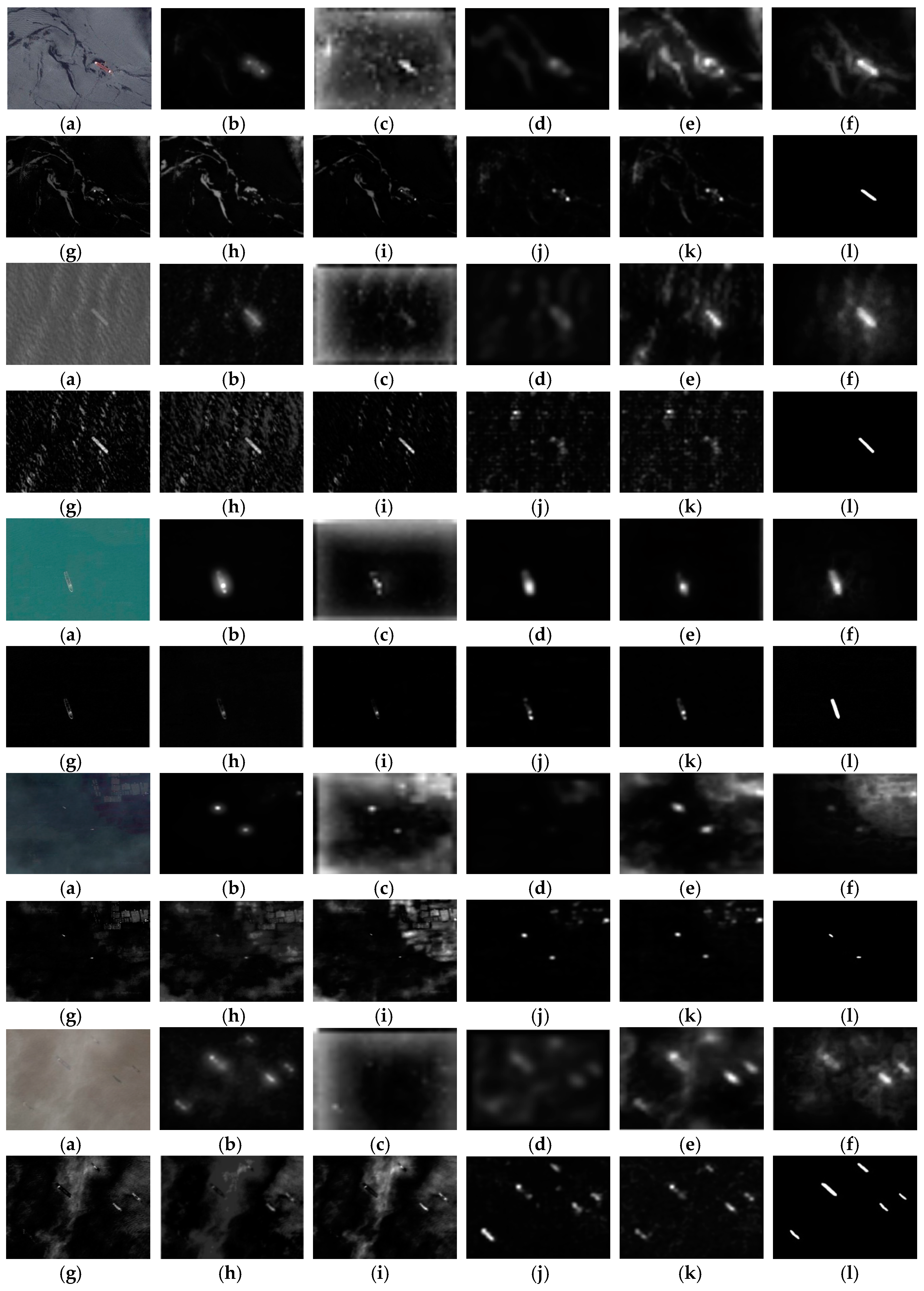
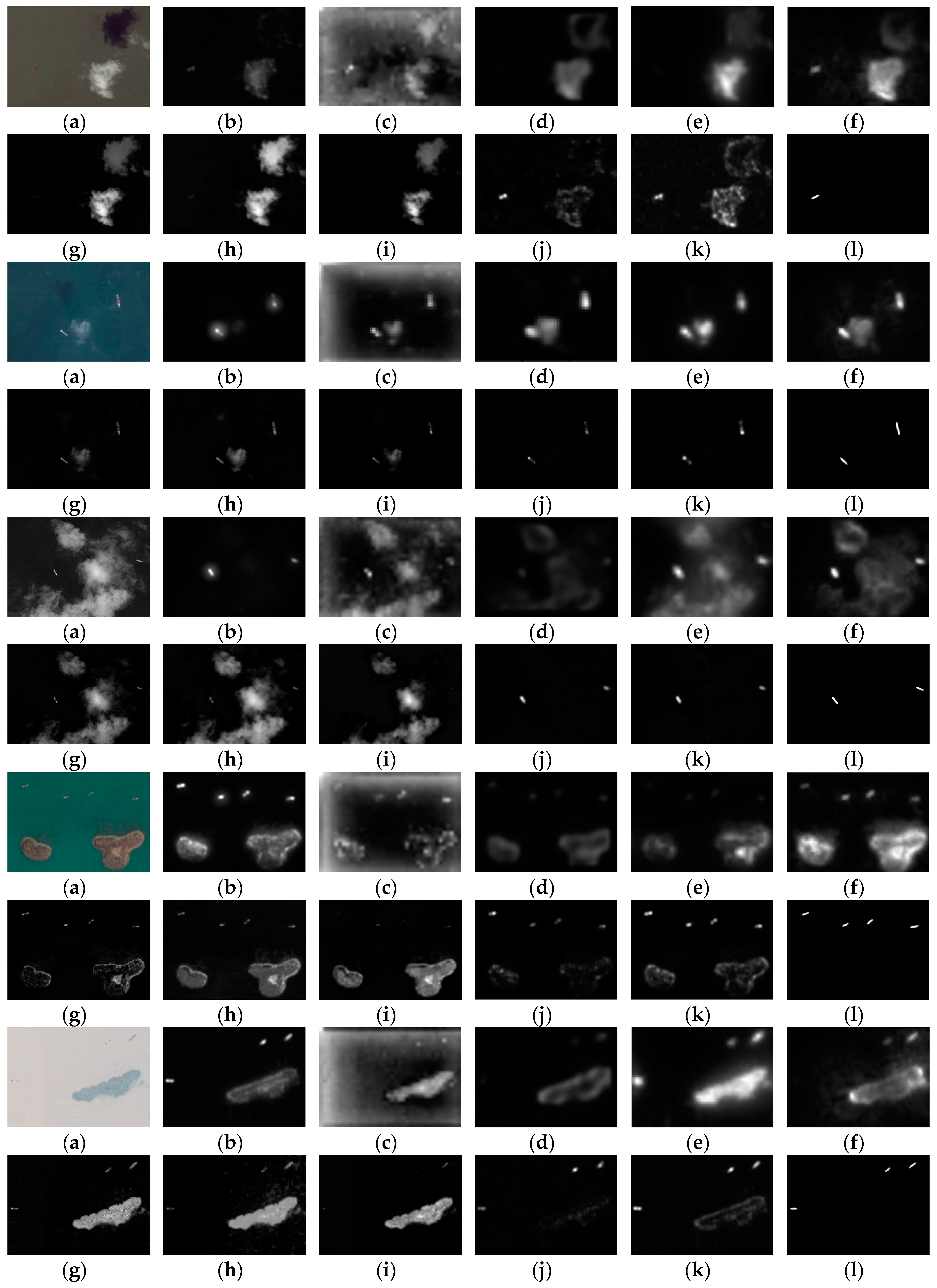
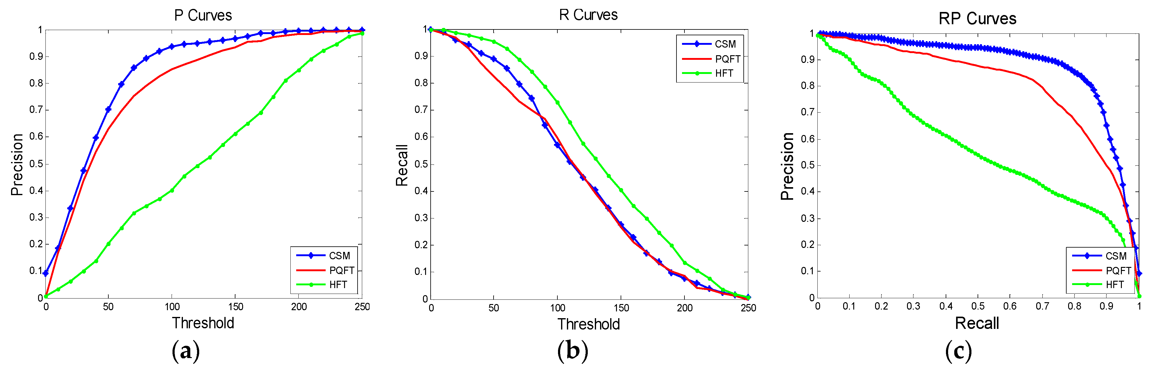
4.1. Comparisons of Different Saliency Models

Figure 11 and Figure 12 illustrate some results of the subjective visual comparison and include ten groups in total. We compare the CSM model with other typical saliency models. Each group has 12 images, including the input image, results of our combined saliency map (CSM) model, results of other models, and a ground-truth map. The ground-truth map refers to the accuracy hull of the ship in the input image, which is a binary image and considered as prior information. For an input image, we manually mark its ground-truth map. Figure 11 shows the comparisons of the background suppression abilities of the different models under all types of complex conditions concluding obvious sea clutter, strong sea waves, low contrast, marine cultivation area, and different color ships.

As shown in Figure 11, although the performance of the CSM model is similar to that of the other models for the images with a simple background, the CSM model significantly outperforms the other models over the images with a complex background. It is noted that the background suppression abilities of the models in the spatial domain are weak, as shown in the first, fourth, and fifth groups. Most of the uneven textures from the sea background are still highlighted. In addition, some small and dim ship targets are missed. Compared with the models based on the spatial domain, the models in the frequency domain are more effective in suppressing the background interference. However, they are incapable of detecting ships under strong sea wave conditions or targets that are relatively large. The integrity of the detected targets is poor, and the false alarm rate may be high. Compared with them, the CSM model has better performance in suppressing the sea clutter, mist, and cloud cover. Furthermore, it is better at searching for single or multiple differently sized and colored ships, even with ship wakes. Although SR and PQFT can also suppress the interference from the background, especially for cloud and mist, they do fail in certain cases in which the ship regions are exceedingly bright or dark. As shown in the first, second, third and fifth groups, the ship regions detected with SR and PQFT may be discontinuous and incomplete. Such phenomena are more obvious when the target is relatively large. The ship region of the CSM model is more uniform and its integrity is higher than those of SR and PQFT. Overall, clearer contour and more uniform salient regions can be highlighted, and more accurate shapes can be obtained by the CSM model.

Figure 12 shows the saliency detection results for the images with heavy clouds and islands.

In Figure 12, the five groups conclude dark ship, clouds and shadow, heavy clouds coverage, islands and coastline, and islands and coastline, respectively. As shown in the second and third groups, the CSM model, the PQFT model and the SR model can effectively suppress the clouds and highlight the targets. However, for the ships with uneven distributions that are too bright or too dark, as shown in the second group, the salient regions are discontinuous when using the PQFT or SR models. The integrity of the detection results from the CSM model is superior to those from the other models. For the pseudo-targets that cannot be suppressed in the first, fourth, and fifth groups, they are expected to be detected as completely as possible. This is conducive to subsequent target identification, and the computational time can be reduced because of the low repetition. It is noted that the Goferman model also has a relatively high detection performance, whereas some small and low-contrast regions may be missed. Compared with these models, different scales and colors of ships can be extracted quickly and accurately by the CSM model. In addition, the number of false chips is reduced, and the workload in the stage of target discrimination is cut down greatly.

In addition to visual comparisons of saliency maps, the total computational time is calculated for the CSM model and the other nine state-of-the-art models. All experiments in this paper are implemented using Matlab 2014a and VS 2010. They are carried out on a 3.30 GHz Intel Core-i3 system with 4 GB of RAM operating system. The time consumption of each model is displayed in

Table 1. Comparison of the computational time.

Model	CSM	ITTI	AIM	GBVS	Goferman	LC	HC	FT	SR	PQFT
Time(s)	1.7219	0.7301	12.6740	7.0883	32.5659	0.0085	0.1323	0.2181	0.1395	0.2019
Code	Matlab	Matlab	Matlab	Matlab	Matlab	C++	C++	C++	Matlab	Matlab

.

In Table 1, since the calculation is relatively simple and C++ code is used, the average computing times of models LC and HC are the shortest. Compared with the processing speed of the models in the spatial domain, the speeds of the models in the frequency domain are more time-efficient. However, in terms of the detection effect, these models are weak at background suppression, as shown in their saliency maps. Although the average processing time of the CSM model is 1.7219 s, it achieves the best visual effect. The CSM model is mainly calculated with Matlab code. To achieve higher computation speed, it will be transplanted to C++ with the use of multi-threading operation, as part of our future work.

In addition to the comparisons above, we also employ the Recall and Precision to evaluate the performances of different saliency models. Recall is computed as the ratio of correctly detected salient regions to the ground-truth regions. Precision is calculated as the ratio of correctly detected saliency regions to the detected salient regions from the saliency model. In terms of saliency detection, PQFT, HFT and the CSM model are compared. After obtaining a detected saliency map S, the binary image of the detected saliency map can be obtained by the threshold segmentation, denoted as SS. For an input image, we manually mark its ground-truth map G. We have the following formulas.

$$\mathrm{R}\mathrm{e}\mathrm{call}=\frac{{\displaystyle \sum \mathrm{G}\times SS}}{{\displaystyle \sum \mathrm{G}}}$$

(17)

$$\mathrm{P}\mathrm{r}\mathrm{ecision}=\frac{{\displaystyle \sum \mathrm{G}\times SS}}{{\displaystyle \sum SS}}$$

(18)

Given a saliency map, it is linearized into the [0, 255] range in the first place. Then, a set of binary maps are obtained by varying the segmentation threshold value from 0 to 255. The Recall and Precision fitting curves at each value of the threshold are shown in Figure 13a,b. Furthermore, the Recall versus Precision (RP) curves are shown in Figure 13c and a reliable comparison is provided by these curves.

Based on the comparison in Figure 13c, the PQFT model shows high Precision but relatively poor Recall, which indicates that its background suppression ability is stronger than that of HFT. However, disconnected or incomplete detection regions may appear, and more false alarms may be introduced. The HFT model has better integrity than the PQFT model. The region detected by the HFT model is larger than the target itself, which leads to its low Precision but high Recall. If different targets vary greatly in size, some relatively small and dim ship targets may be missed, which causes decreases in Recall. Compared with these models, the CSM model combines their merits and generates clearer contour and more uniform salient regions. The CSM model clearly outperforms the other models and has a better comprehensive performance.

There is an inverse relationship between Recall and Precision. Recall and Precision scores are not discussed in isolation. After coarse segmentation, F-Measure, the harmonic mean of Precision and Recall, is introduced to evaluate the performance of the saliency model as follows:

$$\mathrm{F}-\mathrm{Measure}=\frac{(1+{\beta }^2)\times \mathrm{P}\mathrm{r}\mathrm{ecision}\times \mathrm{R}\mathrm{ecall}}{{\beta }^2\times \mathrm{P}\mathrm{recision}+\mathrm{R}\mathrm{ecall}}$$

(19)

where β is a positive parameter to determine the importance of Recall over Precision. We set β = 1 in our work to weigh Recall and Precision equally. After obtaining binarized maps, the average values of Precision, Recall, and the F-Measure are calculated. A comparison between the CSM model and the other nine models is given in terms of the three measures in

Table 2. Comparison in terms of the three measures.

Model	CSM	ITTI	AIM	GBVS	Goferman	LC	HC	FT	SR
Recall	0.9506	0.5102	0.4998	0.5718	0.5957	0.3291	0.2952	0.1087	0.6046
Precision	0.6173	0.1482	0.2921	0.4327	0.4944	0.1719	0.1257	0.1001	0.7751
F-Measure	0.7485	0.2297	0.3687	0.4926	0.5403	0.2258	0.1763	0.1042	0.6793

. Note that the overall performance of the CSM model is better than those of other saliency models.

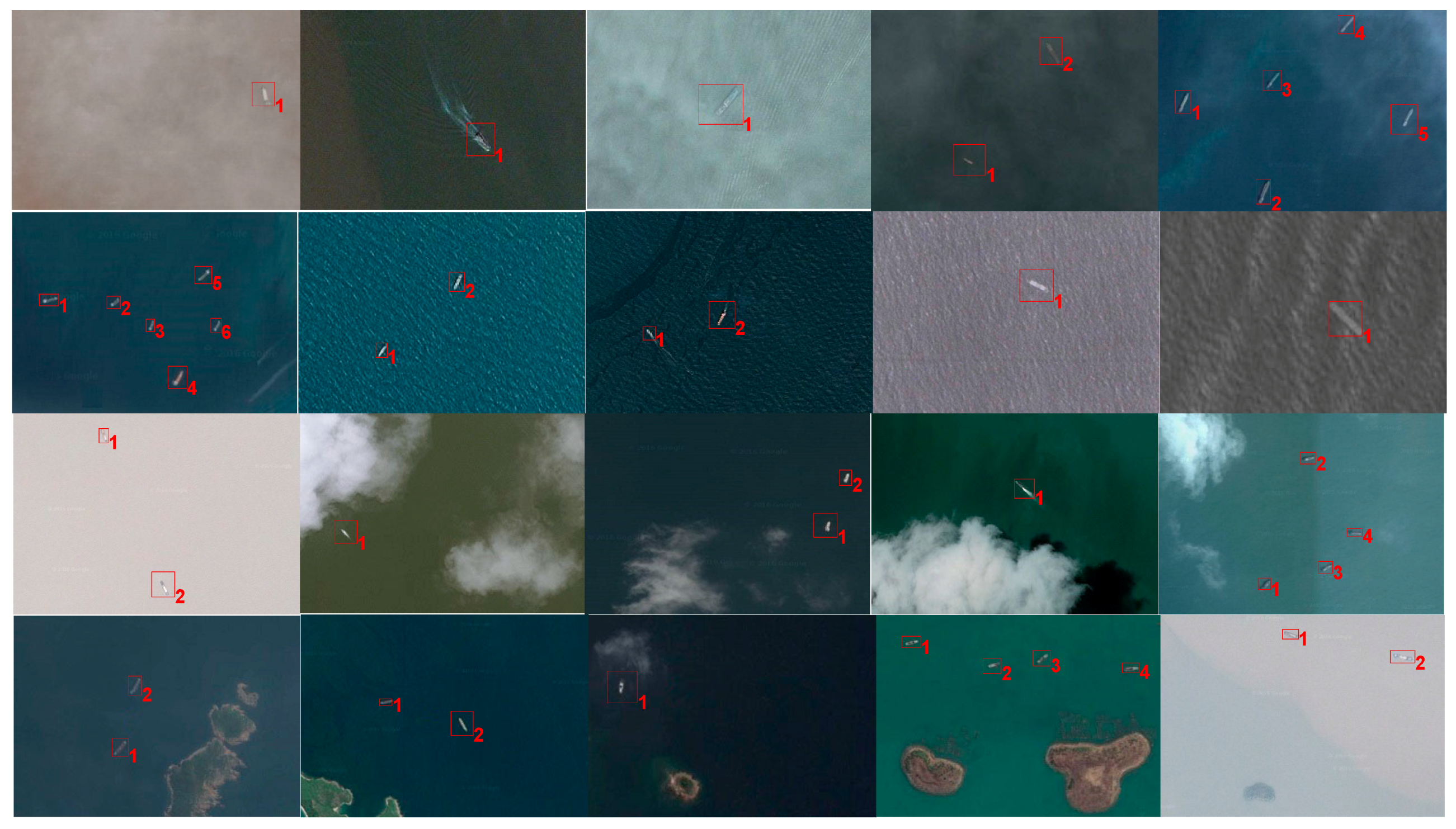
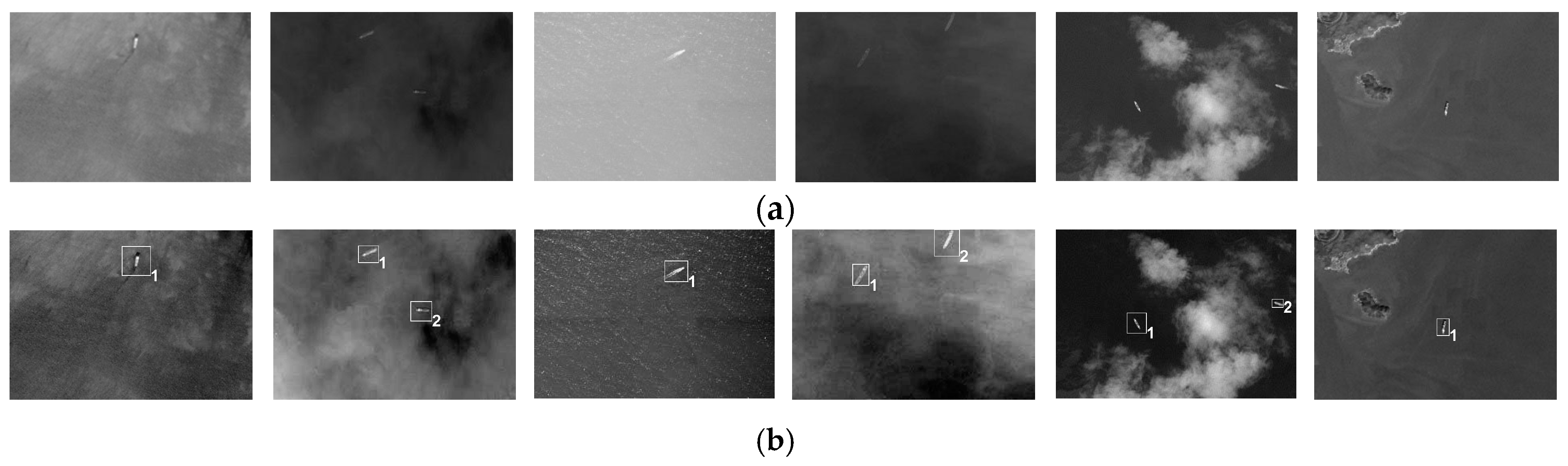
4.2. Discrimination Results

To evaluate the total performance of our method after discrimination, we test it in terms of the accuracy ratio (Cr), missing ratio (Mr), and false alarm ratio (Far), defined as follows:

$$\mathrm{C}r=\frac{Ntt}{Nt}$$

(20)

$$\mathrm{M}r=\frac{Nt-Ntt}{Nt}$$

(21)

$$\mathrm{F}ar=\frac{Nfa}{Ntt+Nfa}$$

(22)

where Nt is the total number of real ships. Ntt is the number of correctly detected ships, and Nfa is the number of false alarms. The detection results are given in

Table 3. Comparison of the results of different methods.

Methods	Nt	Ntt	Nfa	Cr	Far	Mr
				%	%	%
Method [17]	301	239	75	79.402	23.885	20.598
Method [18]	301	256	94	85.049	26.857	14.951
Method [19]	301	254	63	84.385	19.874	15.615
OMWOD	301	288	34	95.681	10.559	4.319
OMWD	301	282	15	93.688	5.050	6.312
OMWODG	301	280	46	93.023	14.11	6.977
OMWDG	301	271	21	90.033	7.192	9.967

. Three unsupervised methods proposed in [17,18,19] are selected for comparison with our method. Our method without discrimination (OMWOD) and our method with discrimination (OMWD) are also compared to test the performance of the gradient feature descriptor. The gray images are tested in addition to the color images and the methods for comparisons are abbreviated as follows: our method without discrimination (OMWODG) and our method with discrimination (OMWDG).

Among the first five methods as listed in Table 3, it is easy to conclude that OMWD can achieve better performance. Most ships are well detected, and the false alarm rate is the lowest. Method [17] suffers from interference introduced in the process of obtaining the ship target. Despite the use of wavelet transform for interference removal, the detection in complex sea backgrounds is still unsatisfying. Method [19] can highlight abnormal signals of ship targets by analyzing the gray level distribution histogram of the sea surface and identify targets based on the compactness and aspect ratio. Compared with method [17], method [19] has superior performance. However, the identification approach used in method [19] is simple and rough. The detection performance is affected greatly in the case of textured sea. For mild sea surfaces, method [18] achieves higher Cr than methods [17,19], while it obtains a poor Cr for complex sea surfaces. This occurs since method [18] lacks final ship identification, whereby the number of false alarms detected would greatly increase. Compared with the three methods above, thin cloud and fog can be suppressed effectively when OMWOD is used exclusively. However, Far is still slightly higher when islands or heavy clouds are present. After the target identification, as a benefit from the characteristics of the gradient feature, the false alarms are greatly eliminated and most real ships are well identified. The Far of OMWD obviously decreased. When the last two methods are tested on gray images, the total detection performance of OMWODG and OMWDG slightly dropped compared with the test results on color images. The reason lies in the representation ability of the original Lab features being better than that of the synthetic three-channel color features, which may cause more false alarms. It is noted that the Cr values of OMWD and OMWDG are slightly lower than those of OMWOD and OMWODG. The reason for this would be that the shape of the ship target may be irregular and incomplete after fine segmentation, which may cause errors in identifying the target and result in some real ships being missed. However, the Far values of OMWD and OMWDG decreased greatly. Through this comprehensive analysis and comparison, we conclude that the total detection performances are improved in OMWD and OMWDG.

In addition, for a ship chip with size 60 × 51, the average running times of coarse segmentation, fine segmentation, Radon transform and gradient feature are 0.062, 0.011, 0.149 and 0.158 s, respectively. In Figure 14, a set of detection examples are displayed, where, most false alarms are removed, whereas the real ship targets are extracted after the discrimination. The regions containing real ships are marked with red boxes.

Some detection results for gray images are shown in Figure 15. The first row contains gray images. The second row contains their corresponding synthetic RGB images and their detection results. The ships are detected and marked with white boxes. It is noted that the number and the locations of ships are determined accurately.

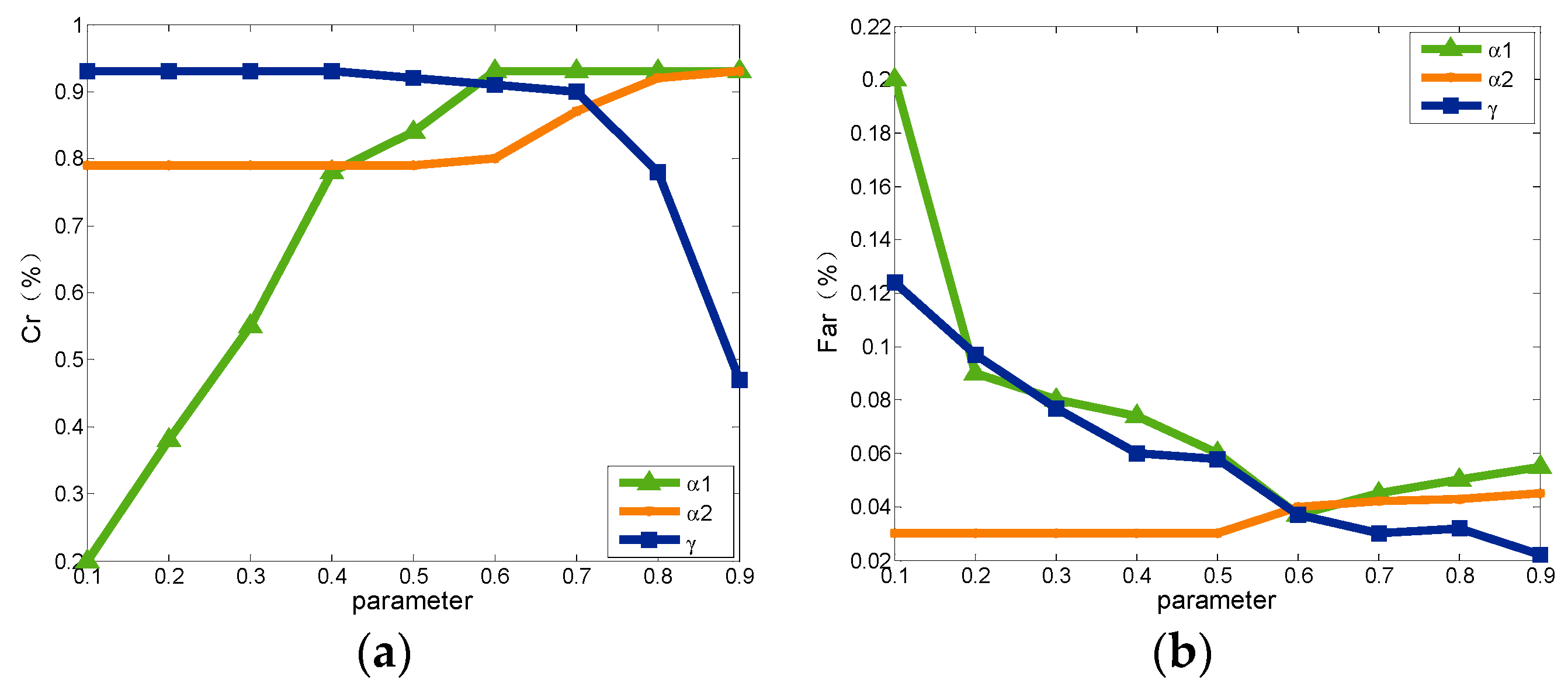
4.3. Selection of Relaxation Parameters

To select appropriate relaxation parameters α1, α2 and γ, the following tests are designed and illustrated. We vary one parameter each time and fix the other two to the aforementioned empirical values. For each set of parameter values, we compute Cr and Far. When α1 is small, the determined condition is strict, and the number of ships correctly discriminated is low. The corresponding Cr is small. As a result of the high number of false alarms, Far is high. With the increase in α1, the criterion is relaxed. Cr increases, and Far decreases. When α1 is very large, the number of false alarms is high, and Far increases. γ reflects magnitude deviation between h1 and h5. If γ changes are smaller, the determined constraint is more relaxed; otherwise, the condition is stricter. The Cr value increases with the increase in γ, while Far decreases. α2 reflects the details of the conditions and has little effect on the experimental result. Its value is affected by parameter γ. These three parameters are set to the empirical values, which better balance the two indicators Cr and Far. The relationship curves are shown in Figure 16. Based on the analysis above, the parameters are set to the following values after the test: α1 = 0.6, α2 = 0.7 and γ = 0.65.

5. Conclusions

In this paper, a new hierarchical framework is proposed for detecting and extracting ships from optical remote sensing images, which includes saliency model improvement, fusion modification with a self-adaptive threshold and target discrimination. To highlight ship targets against a complex sea background, we improved the HFT model and PQFT model in terms of the color, frequency domain transform and amplitude information. To generate clearer contour and more uniform salient target regions, a combination of the saliency models is constructed which fuses the merits of the two models through a self-adaptive threshold based on Entropy information. False alarms are effectively suppressed by using our combined saliency map (CSM) model, whereas most real ship targets are well preserved. Furthermore, to eliminate heavy clouds, islands, and possible false alarms, a novel descriptor based on gradient features is introduced to characterize the ship target. As the outcome, our method achieves robustness against scenes with clouds, islands and sea clutter and is effective in the presence of ship size variation and ship wakes. Furthermore, it is effective not only for color images but also gray images. Quality evaluations, both subjective and objective, of the detection performance are executed. Compared with state-of-the-art methods, our method reaches relatively high detection accuracy. In addition, it ensures a fairly low false alarm rate. Through optimization, the extraction of ship targets on large sea area can be completed quickly. Combined with the altitude information of Unmanned Airborne Vehicle (UAV) or satellite platforms, our method can further calculate the positions or headings of ships. Moreover, our method also lays the foundation for the classification and recognition of ship targets. There is certain significance in civil and military applications.

However, segmentation is difficult in cases with very low-contrast and blurry sea backgrounds. The accuracy of segmentation of the ship hulls affects the identification performance in the discrimination stage. Thus, our main objective will be to improve the performance of segmentation and to thereby ensure high accuracy in target extraction. In addition, the deep neural network (DNN) presented by Tang [54] has become increasingly attractive, and we plan to seek possible use of it on multimodal object detection and recognition. Owing to the difficulty of constructing the DNN and the database of various ship targets, this will be left for future research.

References

1. Mirghasemi, S.; Yazdi, H.S.; Lotfizad, M. A target-based on color space for sea target detection. Appl. Intell. 2012, 36, 960–978. [Google Scholar] [CrossRef]
2. Brusch, S.; Lehner, S.; Fritz, T.; Soccorsi, M.; Soloviev, A.; Schie, B.V. Ship surveillance with TerraSAR-X. IEEE Trans. Geosci. Remote Sens. 2011, 49, 1092–1101. [Google Scholar] [CrossRef]
3. Wei, J.J.; Zhang, J.X.; Huang, G.M.; Zhao, Z. On the use of cross-correlation between volume scattering and helix scattering from polarimetric SAR data for the improvement of ship detection. Remote Sens. 2016, 8, 74. [Google Scholar] [CrossRef]
4. Wang, W.G.; Ji, Y.; Liu, X.X. A novel fusion-based ship detection method from Pol-SAR images. Sensors 2015, 15, 25072–25089. [Google Scholar] [CrossRef] [PubMed]
5. Fan, F.Y.; Luo, F.; Li, M.; Hu, C.; Chen, S.L. Fractal properties of autoregressive spectrum and its application on weak target detection in sea clutter background. IET Radar Sonar Navig. 2015, 9, 1070–1077. [Google Scholar] [CrossRef]
6. Tello, M.; López-Martínez, C.; Mallorqui, J.J. A novel algorithm for ship detection in SAR imagery based on the wavelet transform. IEEE Trans. Geosci. Remote Sens. Lett. 2005, 2, 201–205. [Google Scholar] [CrossRef]
7. Gómez-Enri, J.; Scozzari, A.; Soldovieri, F.; Coca, J.; Vignudelli, S. Detection and characterization of ship targets using CryoSat-2 altimeter waveforms. Remote Sens. 2016, 8, 193. [Google Scholar] [CrossRef]
8. Scozzari, A.; Gómez-Enri, J.; Vignudelli, S.; Soldovieri, F. Understanding target-like signals in coastal altimetry: Experimentation of a tomographic imaging technique. Geophys. Res. Lett. 2012. [Google Scholar] [CrossRef]
9. Bai, X.Z.; Liu, M.M.; Wang, T.; Chen, Z.G.; Wang, P.; Zhang, Y. Feature based on fuzzy inference system for segmentation of low-contrast infrared ship images. Appl. Soft Comput. 2016, 46, 128–142. [Google Scholar] [CrossRef]
10. Tao, W.B.; Jin, H.; Liu, J. Unified mean shift segmentation and graph region merging algorithm for infrared ship target segmentation. Opt. Eng. 2007. [Google Scholar] [CrossRef]
11. Wu, J.W.; Mao, S.Y.; Wang, X.P.; Zhang, T.X. Ship target detection and tracking in cluttered infrared imagery. Opt. Eng. 2011. [Google Scholar] [CrossRef]
12. Liu, Z.Y.; Bai, X.Z.; Sun, C.M.; Zhou, F.G.; Li, Y.J. Infrared ship target segmentation through integration of multiple feature maps. Image Vis. Comput. 2016, 48, 14–25. [Google Scholar] [CrossRef]
13. Graziano, M.D.; D’Errico, M.; Rufino, G. Wake component detection in X-band SAR images for ship heading and velocity estimation. Remote Sens. 2016, 8, 498. [Google Scholar] [CrossRef]
14. Heiselberg, H. A direct and fast methodology for ship recognition in Sentinel-2 multispectral imagery. Remote Sens. 2016, 8, 1033. [Google Scholar] [CrossRef]
15. Jeong, S.; Ban, W.S.; Choi, S.; Lee, D.H.; Lee, M. Surface ship-wake detection using active sonar and one-class support vector machine. IEEE J. Ocean. Eng. 2012, 37, 456–466. [Google Scholar] [CrossRef]
16. Burgess, D.W. Automatic ship detection in optical satellite multispectral imagery. Photogramm. Eng. Remote Sens. 1993, 59, 229–237. [Google Scholar]
17. Corbane, C.; Najman, L.; Pecoul, E.; Demagistri, L.; Petit, M. A complete processing chain for ship detection using optical satellite imagery. Int. J. Remote Sens. 2010, 31, 5837–5854. [Google Scholar] [CrossRef]
18. Proia, N.; Pagé, V. Characterization of a Bayesian ship detection method in optical satellite images. IEEE Trans. Geosci. Remote Sens. 2010, 7, 226–230. [Google Scholar] [CrossRef]
19. Yang, G.; Li, B.; Ji, S.F.; Gao, F.; Xu, Q.Z. Ship detection from optical satellite images based on sea surface analysis. IEEE Trans. Geosci. Remote Sens. 2014, 11, 641–645. [Google Scholar] [CrossRef]
20. Xu, Q.Z.; Li, B.; He, Z.F.; Ma, C. Multiscale contour extraction using level set method in optical satellite images. IEEE Trans. Geosci. Remote Sens. Lett. 2011, 8, 854–858. [Google Scholar] [CrossRef]
21. Corbane, C.; Marre, F.; Petit, M. Using SPOT-5 data in panchromatic mode for operational detection of small ships in tropical area. Sensors 2008, 8, 2959–2973. [Google Scholar] [CrossRef] [PubMed]
22. Zhu, C.R.; Zhou, H.; Wang, R.S.; Guo, J. A novel hierarchical method of ship detection from spaceborne optical image based on shape and texture features. IEEE Trans. Geosci. Remote Sens. 2010, 48, 3446–3456. [Google Scholar] [CrossRef]
23. Xia, Y.; Wan, S.H.; Yue, L.H. A novel algorithm for ship detection based on dynamic fusion model of multi-feature and support vector machine. In Proceedings of the 6th International Conference on Image and Graph (ICIG 2011), Hefei, China, 12–15 August 2011.
24. Kumar, S.S.; Selvi, M.U. Sea object detection using colour and texture classification. Int. J. Comp. Appl. Eng. Sci. 2011, 1, 59–63. [Google Scholar]
25. Shi, Z.W.; Yu, X.R.; Jiang, Z.G.; Li, B. Ship detection in high-resolution optical imagery based on anomaly detector and local shape feature. IEEE Trans. Geosci. Remote Sens. 2014, 52, 4511–4523. [Google Scholar]
26. Duan, H.B.; Gan, L. Elitist chemical reaction optimization for contour-based target recognition in aerial images. IEEE Trans. Geosci. Remote Sens. 2015, 53, 2845–2859. [Google Scholar] [CrossRef]
27. Sun, H.; Sun, X.; Wang, H.Q.; Li, Y.; Li, X.J. Automatic target detection in high-resolution panchromatic satellite imagery based on supervised image segmentation. IEEE Trans. Geosci. Remote Sens. Lett. 2012, 9, 109–113. [Google Scholar] [CrossRef]
28. Cheng, G.; Han, J.W.; Zhou, P.C.; Guo, L. Multi-class geospatial object detection and geosgraphic image classification based on collection of part detectors. ISPRS J. Photogramm. Remote Sens. 2014, 98, 119–132. [Google Scholar] [CrossRef]
29. Cheng, G.; Han, J.W.; Guo, L.; Qian, X.L.; Zhou, P.C.; Yao, X.W.; Hu, X.T. Object detection in remote sensing imagery using a discriminatively trained mixture model. ISPRS J. Photogramm. Remote Sens. 2013, 85, 32–43. [Google Scholar] [CrossRef]
30. Cheng, G.; Han, J.W. A survey on object detection in optical remote sensing images. ISPRS J. Photogramm. Remote Sens. 2016, 117, 11–28. [Google Scholar] [CrossRef]
31. Han, J.W.; Zhou, P.C.; Zhang, D.W.; Cheng, G.; Guo, L.; Liu, Z.B.; Bu, S.H.; Wu, J. Efficient, simultaneous detection of multi-class geospatial targets based on visual saliency modeling and discriminative learning of sparse coding. ISPRS J. Photogramm. Remote Sens. 2014, 89, 37–48. [Google Scholar] [CrossRef]
32. Yokoya, N.; Iwasaki, A. Object detection based on sparse representation and Hough voting foroptical remote sensing imagery. IEEE J. Sel. Top. Appl. Obs. Remote Sens. 2015, 8, 2053–2062. [Google Scholar] [CrossRef]
33. Wang, X.; Shen, S.Q.; Ning, C.; Huang, F.C.; Gao, H.M. Multi-class remote sensing object recognition based on discriminative sparse representation. Appl. Opt. 2016, 55, 1381–1394. [Google Scholar] [CrossRef] [PubMed]
34. Bi, F.K.; Zhu, B.C.; Gao, L.N.; Bian, M. A visual search inspired computational model for ship detection in optical satellite images. IEEE Trans. Geosci. Remote Sens. Lett. 2012, 9, 749–753. [Google Scholar]
35. Zhu, J.; Qiu, Y.; Zhang, R.; Huang, J.; Zhang, W. Top-down saliency detection via contextual pooling. J. Sign. Process. Syst. 2014, 74, 33–46. [Google Scholar] [CrossRef]
36. Itti, L.; Koch, C.; Niebur, E. A model of saliency-based visual attention for rapid scene analysis. IEEE Trans. Patt. Anal. Mach. Intell. 1998, 20, 1254–1259. [Google Scholar] [CrossRef]
37. Bruce, N.D.; Tsotsos, J.K. Saliency based on information maximization. Adv. Neural Inf. Process Syst. 2006, 18, 155–162. [Google Scholar]
38. Harel, J.; Koch, C.; Perona, P. Graph-based visual saliency. Adv. Neural Inf. Process Syst. 2006, 19, 545–552. [Google Scholar]
39. Stas, G.; Lihi, Z.M.; Ayellet, T. Context-aware saliency detection. IEEE Trans. Patt. Anal. Mach. Intell. 2012, 34, 1915–1926. [Google Scholar]
40. Zhai, Y.; Shah, M. Visual attention detection in video sequences using spatiotemporal cues. In Proceedings of the 14th ACM international conference on Multimedia, Santa Barbara, CA, USA, 23–27 October 2006.
41. Cheng, M.M.; Zhang, G.X.; Mitra, N.J.; Huang, X.L.; Hu, S.M. Global contrast based salient region detection. IEEE Trans. Patt. Anal. Mach. Intell. 2011, 37, 409–416. [Google Scholar]
42. Achanta, R.; Hemami, S.; Estrada, F.; Süsstrunk, S. Frequency-tuned Salient Region Detection. IEEE Conf. Comput. Vision Patt. Recogn. 2009. [Google Scholar] [CrossRef]
43. Hou, X.D.; Zhang, L. Saliency detection: A spectral residual approach. IEEE Conf. Comput. Vision Patt. Recogn. Minneapolis 2007. [Google Scholar] [CrossRef]
44. Guo, C.L.; Ma, Q.; Zhang, L.M. Spatio-temporal saliency detection using phase spectrum of quaternion Fourier transform. In Proceedings of the 2008 IEEE Conference on Computer Vision and Pattern Recognition, Anchorage, AL, USA, 23–28 June 2008.
45. Ding, Z.H.; Yu, Y.; Wang, B.; Zhang, L.M. An approach for visual attention based on biquaternion and its application for ship detection in multispectral imagery. Neurocomputing 2012, 76, 9–17. [Google Scholar] [CrossRef]
46. Li, J.; Levine, M.D.; An, X.J.; Xu, X.; He, H.G. Visual saliency based on scale-space analysis in the frequency domain. IEEE Trans. Patt. Anal. Mach. Intell. 2012, 35, 1–16. [Google Scholar] [CrossRef] [PubMed]
47. Lin, W.S.; Lee, B.S.; Lau, C.T.; Lin, C.W. Bottom-up saliency detection model based on human visual sensitivity and amplitude spectrum. IEEE Trans. Multimed. 2012, 14, 187–198. [Google Scholar]
48. Haweel, R.T.; El-Kilani, W.S.; Ramadan, H.H. Fast approximate DCT with GPU implementation for image compression. J. Vis. Commun. Image R. 2016, 40, 357–365. [Google Scholar] [CrossRef]
49. Otsu, N. A threshold selection method from gray-level histograms. IEEE Trans. Sys. Man. Cyber. 1979, 9, 62–66. [Google Scholar] [CrossRef]
50. Qi, S.X.; Ma, J.; Lin, J.; Li, Y.S.; Tian, J.W. Unsupervised ship detection based on saliency and S-HOG descriptor from optical satellite images. IEEE Trans. Geosci. Remote Sens. Lett. 2015, 12, 1451–1455. [Google Scholar]
51. Xu, C.; Zhang, D.P.; Zhang, Z.N.; Feng, Z.Y. BgCut: automatic ship detection from UAV images. Sci. World J. 2014, 171978, 1–11. [Google Scholar] [CrossRef] [PubMed]
52. Margarit, G.; Tabasco, A. Ship classification in single-pol SAR images based on fuzzy logic. IEEE Trans. Geosci. Remote Sens. 2011, 49, 3129–3138. [Google Scholar] [CrossRef]
53. Song, S.L.; Xu, B.; Yang, J. SAR target recognition via supervised discriminative dictionary learning and sparse representation of the SAR-HOG feature. Remote Sens. 2016, 8, 683. [Google Scholar] [CrossRef]
54. Tang, J.X.; Deng, C.W.; Huang, G.B.; Zhao, B.J. Compressed-domain ship detection on spaceborne optical image using deep neural network and extreme learning machine. IEEE Trans. Geosci. Remote Sens. 2015, 53, 1174–1185. [Google Scholar] [CrossRef]
Figure 1. Diagram of the proposed ship detection scheme.
Remotesensing 09 00280 g001
Figure 2. Saliency estimation of ship target in the first stage.
Remotesensing 09 00280 g002
Figure 3. Image represented by quaternions.
Remotesensing 09 00280 g003
Figure 4. Comparisons between the original and the improved models. (a) Input images. (b) Original model: (from left to right): Hypercomplex Frequency Domain Transform (HFT), HFT, Phase Quaternion Fourier Transform (PQFT), PQFT. (c) Improved model: (from left to right): HFT, HFT, PQFT, PQFT.
Remotesensing 09 00280 g004
Figure 5. Visual comparisons of saliency maps.
Remotesensing 09 00280 g005
Figure 6. The transformation process.
Remotesensing 09 00280 g006
Figure 7. Ship target region extraction and marking.
Remotesensing 09 00280 g007
Figure 8. Some fine segmentation results: (a) ship chips; (b) island chips; (c) cloud chips; (d) other chips.
Remotesensing 09 00280 g008
Figure 9. Rotation and alignment: (from left to right) target chips after fine segmentation, description of θ and θb, Radon transform, results of the transform.
Remotesensing 09 00280 g009
Figure 10. Histogram statistics of the three blocks for eight bins: (from top to down) big ship, small ship, ship with wake, cloud and island.
Remotesensing 09 00280 g010
Figure 11. Visual comparison of saliency maps: (a) input image; (b) CSM; (c) ITTI (devised by Itti et al.); (d) Attention based on Information Maximization (AIM); (e) Graph-Based Visual Saliency (GBVS); (f) Goferman; (g) Linear contrast (LC); (h) Histogram Contrast (HC); (i) Frequency-Tuned Saliency (FT); (j) Spectral Residual (SR); (k) PQFT; (l) ground-truth.
Remotesensing 09 00280 g011
Figure 12. Visual comparison of saliency maps: (a) input image; (b) CSM; (c) ITTI; (d) AIM; (e) GBVS; (f) Goferman; (g) LC; (h) HC; (i) FT; (j) SR; (k) PQFT; (l) ground-truth.
Remotesensing 09 00280 g012
Figure 13. Performance comparison: (a) Precision curves; (b) Recall curves; (c) RP curves.
Remotesensing 09 00280 g013
Figure 14. Detection results after discrimination.
Remotesensing 09 00280 g014
Figure 15. Detection results after discrimination: (a) gray images; (b) synthetic images.
Remotesensing 09 00280 g015
Figure 16. Cr and Far curves for different relaxation parameters: (a) Cr curves; (b) Far curves.
Remotesensing 09 00280 g016