A Combined Random Forest and OBIA Classification Scheme for Mapping Smallholder Agriculture at Different Nomenclature Levels Using Multisource Data (Simulated Sentinel-2 Time Series, VHRS and DEM)

Abstract

Sentinel-2 images are expected to improve global crop monitoring even in challenging tropical small agricultural systems that are characterized by high intra- and inter-field spatial variability and where satellite observations are disturbed by the presence of clouds. To overcome these constraints, we analyzed and optimized the performance of a combined Random Forest (RF) classifier/object-based approach and applied it to multisource satellite data to produce land use maps of a smallholder agricultural zone in Madagascar at five different nomenclature levels. The RF classifier was first optimized by reducing the number of input variables. Experiments were then carried out to (i) test cropland masking prior to the classification of more detailed nomenclature levels, (ii) analyze the importance of each data source (a high spatial resolution (HSR) time series, a very high spatial resolution (VHSR) coverage and a digital elevation model (DEM)) and data type (spectral, textural or other), and (iii) quantify their contributions to classification accuracy levels. The results show that RF classifier optimization allowed for a reduction in the number of variables by 1.5- to 6-fold (depending on the classification level) and thus a reduction in the data processing time. Classification results were improved via the hierarchical approach at all classification levels, achieving an overall accuracy of 91.7% and 64.4% for the cropland and crop subclass levels, respectively. Spectral variables derived from an HSR time series were shown to be the most discriminating, with a better score for spectral indices over the reflectances. VHSR data were only found to be essential when implementing the segmentation of the area into objects and not for the spectral or textural features they can provide during classification.

1. Introduction

Over the next decades, climate change combined with demographic and environmental pressures are expected to have significant effects on livelihoods and food systems, particularly in developing countries where less adaptable, small rainfed agricultural systems are dominant [1]. Nevertheless, such forms of agriculture account for about 50% of rural populations and contribute to roughly 90% of staple food production in developing countries [2]. A sustainable improvement of food security for these farmers and populations requires better monitoring of agricultural systems and of their production at regional and global scales. However, satellite observations of these systems are subject to several constraints such as small field sizes, landscape fragmentation, vast within plot and cultivation practices heterogeneity, cloudy conditions, synchronized agro-system and ecosystem phenologies related to rainfall, etc.

Many attempts have been made to use remote sensing to objectively characterize and monitor agricultural systems at different scales. Remote sensing approaches have been developed to identify cropping systems and practices, such as crop type and cropping intensity, across large spatial and temporal scales [3,4,5,6]. Given their ability to observe cultivated areas on a uniform timescale and cover large areas, time series composed of low spatial resolution (LSR) satellite images that record phenological changes in crop reflectance characteristics have been identified as a particularly appropriate source of information for the estimation of such data [7]. However, existing satellite sources may not be appropriate for mapping cropping practices of smallholder farms, in which fields are typically smaller than the spatial resolution of readily available LSR satellite data, such as MODIS (Moderate Resolution Imaging Spectroradiometer, 250 m resolution) and even medium spatial resolution (MSR) Landsat data (30 m resolution). Using the Pareto Boundary method [8], one study analyzed the optimal accuracy of cropland maps that could theoretically be reached for a broad range of West African agricultural systems [9]. The authors quantified the expected accuracy of different spatial resolutions (from 500 m to 10 m) and showed that a resolution of 10 m allows one to produce very accurate cropland maps, even in smallholder agriculture regions.

After the launch of the second Sentinel-2B satellite in March 2017, the Sentinel-2 mission proposed by the European Space Agency will provide significant improvements from existing Landsat-type sensors with an unprecedented combination of spectral (13 bands), spatial (from 10 to 60 m) and temporal (five day) resolutions over a swath of 290 km (see [10] for more information on the mission). The mission may spur major advances in the mapping of agricultural systems, particularly when methods involve the use of Landsat 8 to increase acquisition frequency levels, which may be needed in countries characterized by frequent cloud coverage. However, such high spatial resolution time series with multiple bands and possible derivations constitute a large volume of data that remains a significant challenge for the automated mapping of agricultural land [11]. An emerging machine learning technique based on the use of ensemble methods (e.g., neural network ensembles, random forests, bagging and boosting) is currently receiving increasing interest [12]. Ensemble classifiers are based on the theory that a set of classifiers gives a more robust outcome than an individual classifier [12]. The ensemble learning technique referred to as Random Forests (RF) [13] is increasingly being applied in land-cover classification using multispectral and hyperspectral satellite sensor imagery [14,15,16,17,18,19,20]. The approach presents many advantages in its application to remote sensing: it is non-parametric, it can manage a large volume of data and variables (even those that are highly correlated), it can measure degrees of variable importance, etc. [12].

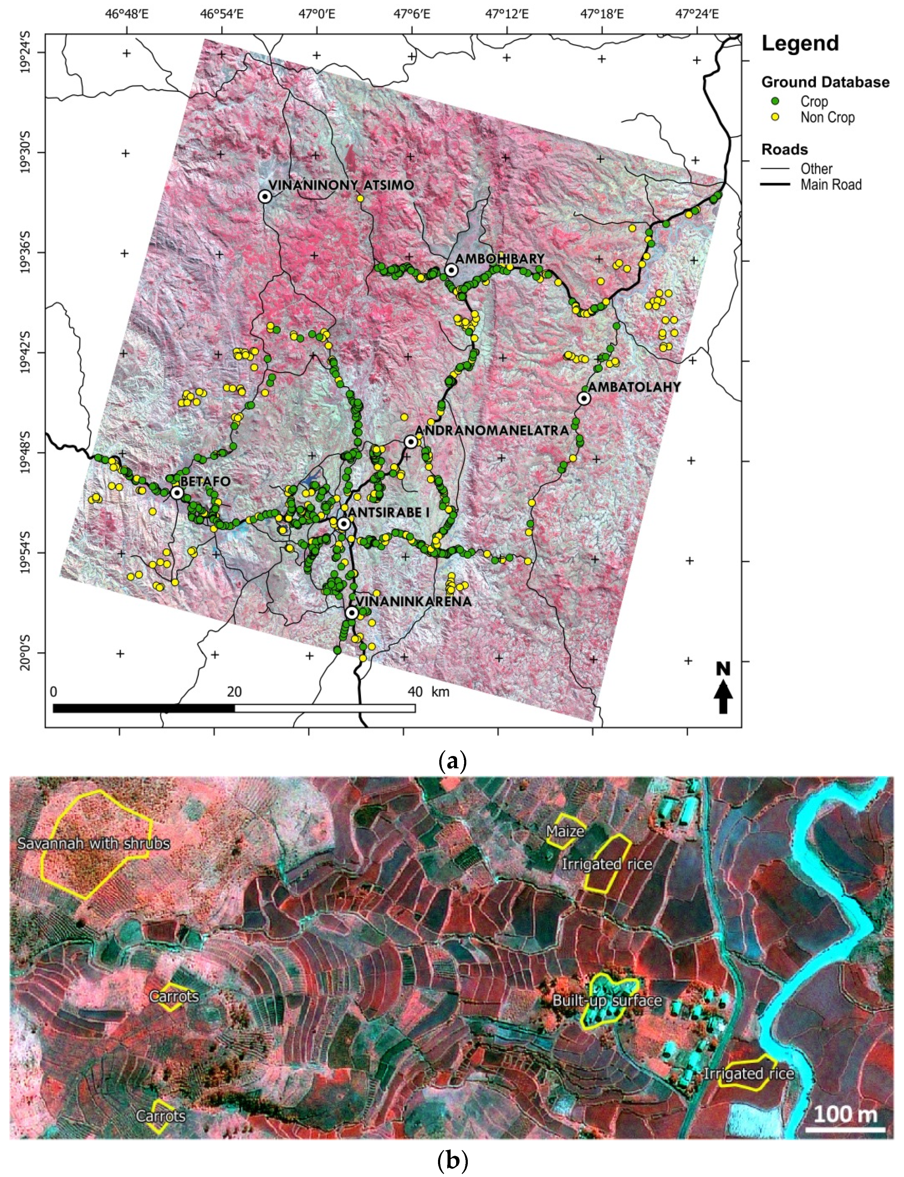
A preparatory work of the Sentinel-2 mission based on such a technique was carried out for the crop type classification of 12 contrasting agricultural sites of the JECAM network (Joint Experiment for Crop Assessment and Monitoring, www.jecam.org), including the Antsirabe site in Madagascar [21,22]. The project was based on a Random Forest analysis of a set of reflectances and spectral indices (Normalized Difference Vegetation Index (NDVI), Normalized Difference Water Index (NDWI) and brightness) extracted at the pixel level, mainly from HRS SPOT4 times series (from the SPOT4 Take5 experiment [23] simulating Sentinel-2). This study highlights the difficulties associated with mapping smallholder agriculture. For sites of intensive farming (France, China, Argentina, Ukraine, etc.), the overall accuracy of classifications of main crop types were always higher than 80%, whereas for sites characterized by smallholder agriculture (JECAM sites in Burkina Faso and Madagascar), the overall accuracies were found to be approximately 50%.

For such complex landscapes, methods could benefit from the addition of very high spatial resolution (VHSR) imagery [24] or from any other satellite-derived environmental information, such as elevation data [20]. Very high spatial resolution images allow one to retrieve field boundaries using segmentation processes [25], thus paving the way for Objects Based Image Analysis (OBIA) [26]. Because per-pixel methods can be affected by mixed pixels, spectral similarities between different crops, and crop pattern variability [27], the OBIA approach already showed many advantages over per-pixel methods, including over agricultural areas [28]. The level of detail provided by VHSR images can also be mobilized in OBIA approaches to calculate textural indices that provide information on the spatial organization of pixels (within a field or between fields, depending on the calculation window size) that is complementary to spectral information [27,29]. Concerning the classification algorithm to be used in an object-based approach for agricultural mapping, a recent study showed the relevance and stability of the RF approach over other supervised classifiers [30].

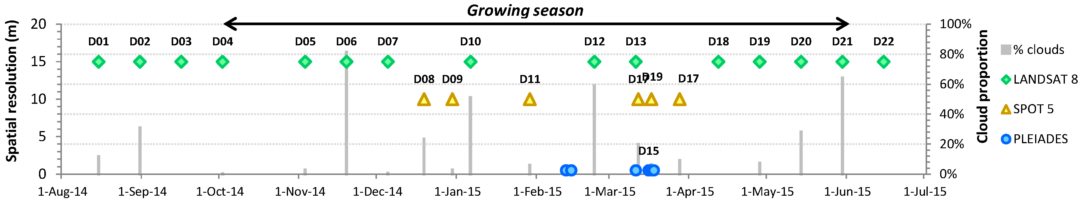
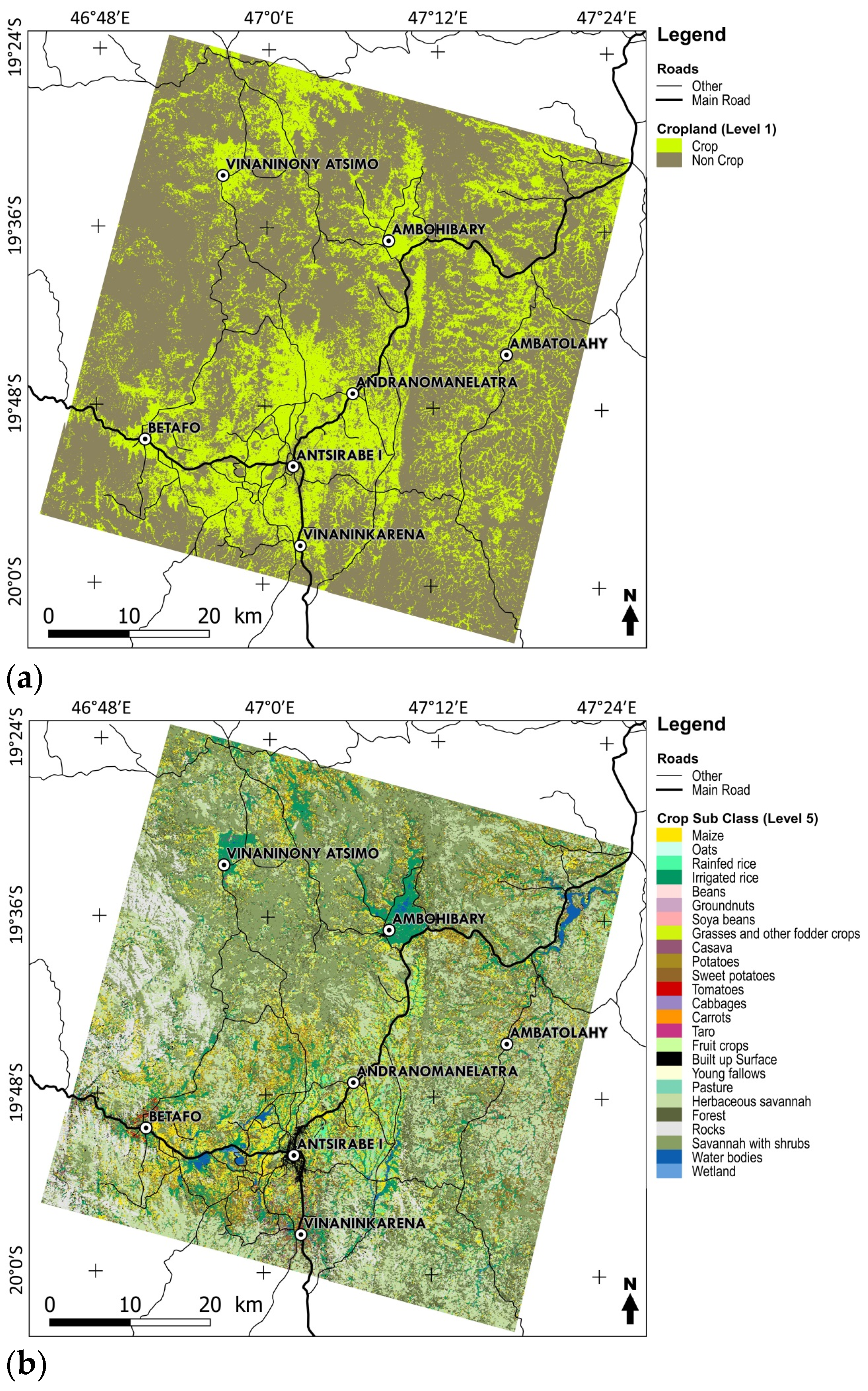
To effectively address the challenges associated with mapping tropical smallholder agricultural systems at a regional scale, the present study aimed at testing the potential of coupling Sentinel-2 data with VHSR and ancillary data (including a Digital Elevation Model—DEM) to map land use, with a focus on agricultural land in the central highlands of Madagascar. The simulation of Sentinel-2 images was based on existing 2014–2015 SPOT 5 and Landsat 8 satellite time series associated with VHSR PLEIADES image coverage. A mixed Random Forest and OBIA classification scheme was developed to combine the HRS time series, VHSR data and ancillary (DEM) data and to achieve a land-use classification at different levels (cropland, land cover, crop group, crop type, and crop subclass). After optimizing the classification approach by reducing the number of features used, we conducted experiments to (i) test cropland masking prior to the classification of more detailed nomenclature levels, (ii) analyze the importance of each data source (HSR, VHRS and DEM) and type (spectral, textural or other), and (iii) quantify their contribution to the classification accuracy. Finally, recommendations are given on ways to perform multisource classifications for mapping smallholder agriculture at different nomenclature levels from cropland to crop subclasses.

2. Materials and Methods

2.1. Study Area and Field Measurements

Madagascar is an island country located in the Indian Ocean off the coast of southeastern Africa. Our 60 km × 60 km study zone belongs to the JECAM network (Joint Experiment for Crop Assessment and Monitoring, http://www.jecam.org/). It is located near Antsirabe, the capital of the Vakinankaratra region, in the central highlands at an average altitude of 1700 m. This region has the second highest population density in the country and is characterized by its mountainous terrain of terraced, rice-growing valleys positioned between grassy hills and rocky outcrops. Therefore, despite its small size, this study area is characterized by heterogeneous landscapes. The local growing season occurs every year between October and June. Local crops are diversified (see nomenclature in

Table 1. Number of polygons per class in the learning database for each level of the JECAM (Joint Experiment for Crop Assessment and Monitoring) nomenclature (grey: cropped, light grey: non-cropped).

Level 1 Cropland		Level 2 Land Cover		Level 3 Crop Group		Level 4 Crop Class		Level 5 Crop Subclass
Crop	1415	Annual crop	1310	Cereals	484	Maize	191	Maize	191
						Oats	23	Oats	23
						Rice	270	Rainfed rice	112
								Irrigated rice	158
				Leguminous	78	Beans	68	Beans	68
						Peas	10	Peas	10
				Oilseed crops	133	Groundnuts	53	Groundnuts	53
						Soya beans	80	Soya beans	80
				Other crops	117	Other crops	19	Other crops	19
						Grasses and other fodder crops	98	Grasses and other fodder crops	98
				Root or tuber crops	287	Casava	62	Casava	62
						Potatoes	97	Potatoes	97
						Sweet potatoes	128	Sweet potatoes	128
				Vegetables and melons	211	Fruit-bearing vegetables	53	Tomatoes	53
						Leafy or stem vegetables	41	Cabbages	34
								Other leafy or stem vegetables	7
						Root bulb or tuberous vegetables	117	Carrots	59
								Onions (incl. Shallots)	10
								Taro	48
		Ligneous crop	105	Fruit crops	105	Fruit crops	105	Fruit crops	105
Non Crop	899	Built-up surface	79	Built-up Surface	79	Built-up Surface	79	Built-up Surface	79
		Fallows	68	Old fallows	16	Old fallows	16	Old fallows	16
				Young fallows	52	Young fallows	52	Young fallows	52
		Natural spaces	677	Bare soils	16	Bare soils	16	Bare soils	16
				Grassland	225	Pasture	49	Pasture	49
						Herbaceous savannah	176	Herbaceous savannah	176
				Forest	151	Forest	151	Forest	151
				Rocks	84	Rocks	84	Rocks	84
				Shrub land	201	Savannah with shrubs	201	Savannah with shrubs	201
		Water bodies	48	Water bodies	48	Water bodies	48	Water bodies	48
		Wetland	27	Wetland	27	Wetland	27	Wetland	27

), although maize and rice predominate. The area is also known for fruit production. The mean size of an agricultural field in the area is very small (about 0.05 ha), but contiguous fields of the same crop type occasionally give rise to larger crop patches. Rice is mainly grown in irrigated basins but has over the past ten years mingled with other rainfed crops on slopes (called tanetys). This characterizes the agricultural landscape as having: (i) a rather homogeneous irrigated domain consisting of contiguous rice fields that are quite large (relative to the mean field size of the area); and (ii) a highly fragmented rainfed area consisting of a patchwork of very small fields of different crops that are occasionally associated with a second crop and are often surrounded by natural vegetation with a phenology similar to that of the crops grown. Therefore, rainfed areas are very difficult to characterize with satellite imagery.

Fields surveys were conducted in the study zone during the growing peak (end of February and March) of the 2014–2015 cropping season to characterize major cropping systems. GPS waypoints were registered in the study area following an opportunistic sampling approach. The waypoints were chosen according to their accessibility (due to heavy rains some parts of the area could not be reached), the size of the field (at least 20 m wide) and representativeness of existing cropping systems. Data gathered during the field surveys concerned land uses and were recorded at different levels of detail (cropland, land cover, crop group, crop class, and crop subclass) according to JECAM nomenclature (see Table 1). For mixed-crop fields, the main crop was recorded. GPS waypoints were also registered for different types of non-cropped classes (natural vegetation, urban areas, water bodies, etc.) to obtain data on the non-crop class. In addition, 199 points were added to the field database for the non-crop class via photo interpretation of very high resolution PLEIADES imagery, generating a total of 1219 usable points (860 cropped and 359 non-cropped). The boundaries of the fields (cropped classes)/objects (non-cropped classes) were then digitized over very high resolution PLEIADES imagery (0.5 m × 0.5 m pixel size) to obtain a ground polygon database (Figure 1b). A map of GPS waypoints acquired over the 2014–2015 growing season is presented in Figure 1b.

2.2. Earth Observation Data Acquisition and Preprocessing

The satellite data used consisted of a time series of high spatial resolution images (6 SPOT 5 images and 15 Landsat 8 OLI/TIRS) acquired from August 2014 to June 2015 and a very high spatial resolution coverage (PLEIADES) was acquired around the peak of the growing season (March 2015). Due to frequent cloudy conditions, 6 acquisition dates were needed to cover the entire study zone with VHSR PLEIADES imagery (acquired in 20 km × 20 km tiles). 16th March 2015 (D15 for date fifteen) was considered as the central date for the VHSR coverage. Figure 2 presents a chronogram of the 22 satellite acquisitions and the cloud proportion for each date.

PLEIADES images were delivered at the Ortho level (orthorectified in UTM WGS84 Zone 38S) by CNES (Centre National d’Études Spatiales - French Space Agency). They served as a reference for the orthorectification of SPOT 5 images acquired from the SEAS-OI receiving station (Survey of the Environment Assisted by Satellite in the Indian Ocean) on Reunion Island and delivered at level 1A. Landsat 8 images were downloaded from the USGS (United States Geological Survey) Earth Explorer tool at level 1T (Terrain Corrected) of the same projection. All image values were also converted to Top Of Atmosphere (TOA) reflectance.

Landsat 8 images were pansharpened using the Gram–Schmidt pansharpening module [31] of the ENVI 5.0^® software (Harris Geospatial Solutions, Toulouse, France) to obtain a 15 m spatial resolution and were then resampled at 10 m to fit a SPOT 5 10 m spatial resolution. PLEIADES images were also pansharpened, but using the Orfeo ToolBox (OTB, CNES, Toulouse, France) Bundle to perfect sensor tool [32] in order to obtain multispectral information at a 0.5 m spatial resolution. For Landsat 8 images, clouds were masked using fmask (cloud and shadow mask) provided through the Landsat CDR Products and were completed manually. For all other images, clouds were masked manually.

A SPOT Digital Elevation Model (SPOT DEM) was also acquired with absolute horizontal and vertical accuracies of less than 15 m and 10 m, respectively.

2.3. Classification Approach

The classification approach involved three main steps: (i) the segmentation of the whole study zone into objects, (ii) feature extraction to build a learning database, and (iii) using the learning database to train RF and obtaining an optimized classifier for each nomenclature level.

Based on this approach, various experiments were carried out:

-

a hierarchical approach was used (first, crop and non-crop domains at level 1 are isolated and land use is classified by correspondence to each domain for the following nomenclature levels) as opposed to a classical approach (the whole learning database is used at each level);

-

analysis of the importance of the variables according to their source (HRS time series, VHSR image, and ancillary) and their types (reflectances, spectral indices, textures, and ancillary);

-

analysis of the contribution of the different data sources and types to the classification accuracy.

The 3 steps of the classification approach and experiments are detailed in the following section.

2.3.1. Segmentation

Our approach involved the use of OBIA, meaning that basic processing units were objects generated through a segmentation algorithm. We used the algorithm proposed by [33] and implemented it through the Trimble eCognition Developer^® 9 platform (Trimble, Munich, Germany). This multiresolution segmentation algorithm generates objects according to a scale parameter (influencing object sizes) using the weights of each spectral band of images being segmented, thematic layers (which lead to additional splitting of image objects according the thematic layer used), and a homogeneity criterion (shape and compactness) [34].

The segmentation process was applied to the four spectral bands of pansharpened 0.5 m PLEIADES images by using a weight of 1 for each band. A scale parameter of 90 was chosen and for the homogeneity criterion, the shape was fixed at 0.1 and the compactness was set at 0.5. These parameters were determined empirically by testing various segmentation settings and by analyzing the segmentation results over different parts of the study zone to determine the boundaries of cultivated fields or homogenous groups of fields within the agricultural area. Thematic layers corresponding to the ground polygon database, and to cloud masks of each time series date, were also used to constrain the segmentation. The process was tiled (into 52 tiles) for a processing facility.

Using cloud masks as an input in the segmentation process and dividing the study zone into 52 tiles resulted in the splitting of a significant number of polygons of the ground database. This resulted in a final population of 2314 polygons in the ground database (1415 crop and 899 non-crop). Table 1 presents the population of polygons per class type for each level of the JECAM nomenclature.

2.3.2. Building a Learning Database

Several variables were calculated from the time series of 22 images (6 SPOT 5, 15 Landsat 8 and 1 PLEIADES) and the DEM and were associated with polygons corresponding to the ground samples. These variables are described in

Table 2. Description of the variables extracted to build the learning database according to their type (reflectances, spectral indices, textures, and ancillary) and source (high spatial resolution imagery (HSR), very high spatial resolution imagery (VHSR), and ancillary).

Variable Source/Type	HSR	VHSR	Ancillary
Reflectances	Mean and standard deviation in green, red, near infrared (NIR) and short wave infrared (SWIR) bands	Mean and standard deviation in blue, green, red, NIR and panchromatic bands
Spectral indices	Mean and standard deviation of NDVI * [35], Brightness index **, NDWI *** [36], MNDWI **** [37]	Mean and standard deviation of NDVI * and Brightness index **
Textural indices		Mean and standard deviation of correlation, contrast, dissimilarity, entropy and variance Haralick indices [38] calculated at five windows sizes (5 × 5, 9 × 9, 17 × 17, 21 × 21, and 35 × 35)
Ancillary			mean and standard deviation of altitude and slope, object size

* Normalized Difference Vegetation Index. ** square root of the sum of squared values in green, red, near infrared (NIR) and short wave infrared (SWIR) bands. *** Normalized Difference Water Index. **** Modified Normalized Difference Water Index.

. They concerned 4 types of variables: reflectances (178 variables), spectral indices (108 variables), textural indices (50 variables) and ancillary variables (5 variables). The textural indices were calculated from the near infrared (NIR) band of the pansharpened PLEIADES. We made the assumption that textures calculated from this band will highlight pixel organizations related to the soil-vegetation discontinuity that are more contrasted in the NIR.

This generated a total of 341 variables: 273 derived from HSR time series, 63 derived from VSHR data, and 5 derived from ancillary variables. The 2314 ground polygons associated with the 341 descriptive satellite variables are hereafter referred to as the learning database.

2.3.3. Building the Optimized Random Forest Classifiers

• Random Forest description and training

RF is an ensemble learning technique that generates a multitude of random decision trees that are then aggregated to compute a classification [13]. In land cover classification studies, the RF classifier has been found to be stable and relatively efficient, to involve few user-defined parameters and to yield overall accuracy levels that are either comparable to or better than other classifiers such as maximum likelihood and conventional decision trees [17], AdaBoost decision trees and neural networks [14], and support vector machines [18]. RF uses a bagging-based approach (random sampling with replacement) to build a forest of classification trees. Each classification tree (500 trees in a typical forest) is constructed from a randomly sampled set consisting of approximately 63% (one third) of the full dataset [39]. Observations of the original dataset that are not found in a bootstrap sample are referred to as out of bag observations (OOB). The OOB of error is calculated using a one-third portion of the data that was randomly excluded from the construction of each of the 500 classification trees and corresponds to the rate of misclassified samples. Consequently, the classification accuracy is estimated internally and does not require an independent validation set [13]. All ground samples can thus be used for RF training, which can be important in study areas where ground data can be difficult to gather.

Of results generated via the RF approach, the mean decrease in accuracy (MDA) for a variable allows one to assess the importance (the degree to which a variable is discriminant) of each variable used for classification. The MDA caused by a variable is determined at the out of bag error calculation phase. The more the accuracy of the RF decreases due to the exclusion (or permutation) of a single variable, the more important that variable is. Consequently, higher values of MDA indicate variables that are more important to the classification [39].

RF was trained at each nomenclature level using the entire learning database (see Table 1) to obtain classifiers at different nomenclature levels. To do so, the randomForest package [40] available through the R software 3.2.5 [41] was used. The minimum population required for the learning database of a given class was set to 20. Below this value, classes were eliminated. Values missing due to the presence of clouds at a given date were filled in using the na.roughfix function of the randomForest package, which imputes missing values with the median of the available records of a given variable.

• Optimization (feature selection)

The RF process was optimized by reducing the number of variables used to maximize the variable volume/overall accuracy ratio. This optimization phase was based on an analysis of the influence of the number of important variables (ranked from the more to the less important with the MDA measure) used on the resulting overall classification accuracy. The optimization process was performed using a cross-validated (5-fold) recursive feature elimination (the rfe function) available through the R Caret package [42]. Optimization was carried out with a dual objective: to improve the accuracy of each classifier by identifying variables most useful to the RF algorithm and reducing noise, and to reduce the number of variables extracted for classifier use over the whole study area to shorten processing periods.

• Accuracy evaluation

The accuracy evaluation was performed through the internal RF validation procedure that makes use of all the sample polygons in the database. The performance of the resulting optimized classifiers was estimated from confusion matrices provided through the RF results via the calculation of two measures: the overall accuracy, which corresponds to the total number of correctly classified objects divided by the total number of test objects, and the Cohen’s Kappa, which reflects the difference between actual agreement and agreement expected by chance [43,44].

For a specific class, accuracy was summarized using the f1-score, which was calculated as the harmonic mean of producer and user accuracies. Producer and user accuracies are linked to omission error (rate of objects incorrectly omitted) and commission error (rate of objects incorrectly included), respectively.

As the same training set was used to produce the classifiers with both approaches (classical and hierarchical), a McNemar’s test [45] was also performed to evaluate if the difference in accuracy between the two approaches was statistically significant. The test is done from a contingency table presenting the number of samples that are well classified by both approaches, misclassified by both approaches, and misclassified by one of the approaches. It is based on a qui-square statistics (χ²) and computed as follows:

$${\mathsf{\chi }}^2=\frac{{\left(n_{ab}-n_{ba}\right)}^2}{n_{ab}+n_{ba}},$$

(1)

where $n_{ab}$ denotes the number of cases that are wrongly classified by classifier A but correctly classified by classifier B, and $n_{ba}$ denotes the number of cases that are correctly classified by classifier A but wrongly classified by classifier B.

2.3.4. Experiments

Various experiments were performed either to improve classification accuracy and computation time (first experiment) or to outline recommendations on the dataset to be used for land use classifications of heterogeneous agricultural areas (two experiments).

• Classical vs. Hierarchical approach

RF was applied through two approaches: (i) a classical approach that involved using the entire learning database to build RF classifiers at each nomenclature level (from level 1, cropland, to level 5, crop subclass) and (ii) a hierarchical approach that involved separating the data into cropland and non-cropland at level 1 of the nomenclature and then building RF classifiers to discriminate crop classes and non-crop classes within cropland and non-cropland respectively for the following nomenclature levels.

• Analysis of variable importance

Thanks to the MDA measure, satellite variables can be ranked by the extent to which they are informative for the classification. In this part of the study, the 30 most important variables used to classify each level of the nomenclature were analyzed according to the following: (i) their sources, i.e., HSR, VHSR, and ancillary and (ii) their type, i.e., reflectances, spectral indices, textures, and ancillary. The proportion (%) of each source or type of variable present among the 30 most important variables can then be summarized for each nomenclature level.

• Contributions of the different variables to classification accuracy

An experiment was also carried out to analyze the contributions of each source and category of data to the accuracy of the classifications. For each nomenclature level, an optimized RF classification was performed from different datasets as presented in

Table 3. Definitions of the experimental datasets used to analyze contributions of the different sources (high spatial resolution imagery (HSR), very high spatial resolution imagery (VHSR), and ancillary) and types (reflectances, spectral indices, textures, and ancillary) of data on the accuracy of the classifications.

Dataset	HSR	VHSR	Ancillary
All data	Reflectances, Spectral Indices	Reflectances, Spectral Indices, Textures	Ancillary
Dataset 1	Reflectances, Spectral Indices	Reflectances, Spectral Indices	Ancillary
Dataset 2	Reflectances, Spectral Indices		Ancillary
Dataset 3	Reflectances, Spectral Indices
Dataset 4	Reflectances
Dataset 5	Spectral Indices
Dataset 6		Reflectances, Spectral Indices, Textures	Ancillary
Dataset 7		Reflectances, Spectral Indices, Textures

. For each of the 8 datasets, the overall accuracy and Cohen’s Kappa for each level were recorded to determine their impacts on the accuracy.

3. Results

3.1. Optimization

Many variables of our dataset are correlated, redundant or not informative, and their use in the classification does not improve overall accuracy. This is illustrated in Figure 3, which shows that for level 1 (cropland), the overall accuracy level achieved depends on the number of variables used in the classification (variables were previously ranked by order of importance using the MDA measure). Similar accuracy profiles were obtained for each level of the nomenclature. Figure 4 presents the optimal number of variables needed to reach the best overall accuracy level for each domain (crop/non-crop) at each nomenclature level when using a hierarchical approach. Overall, the results show that the optimal number of variables increases with the nomenclature level and degree of complexity. This optimization phase allowed for dividing the number of variables to be extracted for each object by 1.5- to 6-fold depending on the classification level.

3.2. Classical vs. Hierarchical Classification Approaches

At level 1 (cropland), “crop” and “non-crop” classes were classified with an overall accuracy of 91.7% (Cohen’s Kappa 0.82) (

Table 4. The overall accuracy and Cohen’s Kappa obtained via the hierarchical approach for each level of the JECAM nomenclature. Colors along the green to red color gradient denote the accuracy of results from good to poor, respectively.

	Cropland (Level 1)	Land Cover (Level 2)		Crop Group (Level 3)		Crop Class (Level 4)		Crop Subclass (Level 5)
		Crop	Non Crop	Crop	Non Crop	Crop	Non Crop	Crop	Non Crop
Overall Accuracy	91.7%	96.6%	90.7%	70.2%	83.2%	64.1%	81.3%	64.4%	80.2%
Kappa	0.82	0.69	0.75	0.61	0.79	0.59	0.78	0.61	0.76

). An f1-score of 0.93 was observed for the “crop” class, representing a high classification accuracy for this specific class corresponding to the cultivated domain (

Table 5. Class f1-scores obtained via the hierarchical approach. Differences in class f1-scores between the hierarchical and classical approaches at different nomenclature levels are shown in brackets. Positive values are shown in green (the hierarchical approach is superior to the classical approach) and negative values are shown in red (the classical approach is superior to the hierarchical approach).

Level 1 Cropland		Level 2 Land Cover		Level 3 Crop Group		Level 4 Crop Class		Level 5Crop Subclass
Crop	0.93	Annual crop	0.98 (0.067)	Cereals	0.79 (0.065)	Maize	0.63 (0.010)	Maize	0.61 (0.006)
						Oats	0.79 (0.104)	Oats	0.67 (0.123)
						Rice	0.78 (0.054)	Rainfed rice	0.65 (0.040)
								Irrigated rice	0.82 (0.015)
				Leguminous	0.40 (0.067)	Beans	0.56 (−0.008)	Beans	0.54 (−0.027)
						Peas		Peas
				Oilseed crops	0.61 (0.015)	Groundnuts	0.51 (−0.046)	Groundnuts	0.55 (0.023)
						Soya beans	0.67 (−0.026)	Soya beans	0.69 (0.025)
				Other crops	0.69 (0.036)	Other crops		Other crops
						Grasses and other fodder crops	0.76 (0.027)	Grasses and other fodder crops	0.73 (0.048)
				Root or tuber crops	0.66 (0.061)	Casava	0.48 (−0.030)	Casava	0.49 (−0.009)
						Potatoes	0.57 (0.030)	Potatoes	0.57 (0.015)
						Sweet potatoes	0.52 (−0.033)	Sweet potatoes	0.49 (0.029)
				Vegetables and melons	0.57 (−0.001)	Fruit-bearing vegetables	0.58 (−0.017)	Tomatoes	0.64 (−0.009)
						Leafy or stem vegetables	0.44 (−0.024)	Cabbages	0.51 (−0.111)
								Other leafy or stem vegetables
						Root bulb or tuberous vegetables	0.44 (−0.016)	Carrots	0.39 (−0.018)
								Onions (incl. Shallots)
								Taro	0.26 (−0.017)
		Ligneous crop	0.71 (0.065)	Fruit crops	0.82 (0.051)	Fruit crops	0.78 (0.019)	Fruit crops	0.74 (0.057)
Non Crop	0.89	Built-up surface	0.83 (0.031)	Built-up Surface	0.91 (0.004)	Built-up Surface	0.88 (0.044)	Built-up Surface	0.86 (0.037)
		Fallows	0.48 (0.146)	Old fallows		Old fallows		Old fallows
				Young fallows	0.54 (0.147)	Young fallows	0.63 (0.086)	Young fallows	0.53 (0.038)
		Natural spaces	0.94 (0.063)	Bare soils		Bare soils		Bare soils
				Grassland	0.85 (0.042)	Pasture	0.61 (−0.019)	Pasture	0.64 (−0.048)
						Herbaceous savannah	0.82 (0.043)	Herbaceous savannah	0.76 (0.048)
				Forest	0.77 (0.073)	Forest	0.77 (0.076)	Forest	0.70 (0.054)
				Rocks	0.87 (−0.005)	Rocks	0.87 (0.016)	Rocks	0.85 (0.025)
				Shrub land	0.84 (0.033)	Savannah with shrubs	0.84 (0.049)	Savannah with shrubs	0.80 (0.026)
		Water bodies	0.92 (0.037)	Water bodies	0.91 (0.030)	Water bodies	0.92 (0.042)	Water bodies	0.87 (0.030)
		Wetland	0.81 (0.142)	Wetland	0.82 (0.133)	Wetland	0.79 (0.077)	Wetland	0.70 (0.094)

).

For levels 2, 3, 4 and 5, class accuracy levels (f1-score) were calculated using both the classical and hierarchical approaches and were compared using absolute f1-score differences between the two approaches (Table 5). When crop and non-crop classes are considered, the hierarchical approach gives better results than the classical approach, generating f1-score improvements of 100%, 87%, 61% and 70% for levels 2, 3, 4 and 5, respectively. When only crop classes are considered, improvements are less significant (100%, 86%, 43%, and 63%, respectively) but are sufficient to conclude that separating first crop domain from non-crop domain before performing classifications can improve the accuracy of the different classes, regardless of the nomenclature level. The results of the McNemar’s test (

Table 6. Results of the McNemar’s test performed at each nomenclature level between the classical and hierarchical approaches.

Level	${\mathit{n}}_{\mathit{a}\mathit{a}}$	${\mathit{n}}_{\mathit{a}\mathit{b}}$	${\mathit{n}}_{\mathit{b}\mathit{a}}$	${\mathit{n}}_{\mathit{b}\mathit{b}}$	Total	$\mathit{\chi }²$	p-Value
Level 2 (Land Cover)	123	157	9	2025	2314	132.0	<0.001
Level 3 (Crop Group)	498	173	69	1542	2282	44.7	<0.001
Level 4 (Crop Class)	580	134	80	1459	2253	13.6	<0.001
Level 5 (Crop Subclass)	593	119	66	1458	2236	15.2	<0.001

$n_{aa}$ number of samples with wrong classification in both classical and hierarchical approaches; $n_{ab}$ number of samples that are wrongly classified by classical approach but correctly classified by the hierarchical approach; $n_{ba}$ number of samples that are correctly classified by classical approach but wrongly classified by hierarchical approach; $n_{bb}$ number of samples with correct classification in both classical and hierarchical approaches.

), performed for levels 2, 3, 4 and 5 show a significant improvement of the hierarchical approach over the classical one, regardless of the nomenclature level (p-values < 0.001).

The following analyses thus only focus on results obtained using the hierarchical approach. Table 4 presents the classification accuracy of the different nomenclature levels derived from the hierarchical approach. It shows that classes belonging to the non-crop domain were well classified regardless of the nomenclature level involved (overall accuracy > 80%, Cohen’s Kappa > 0.75). For classes belonging to the crop domain, classification accuracy levels decreased from level 3 (crop group) to level 5 (crop subclass) with overall accuracies of 70.2% and 64.4%, respectively. Class f1-scores presented in Table 5 for each level of the nomenclature highlight the strong classification accuracy of classes belonging to the non-crop domain (except for “Young Fallows” and “Pasture” at level 5, crop subclass). Concerning classes belonging to the crop domain, the results are more mixed. For level 2 (land cover), “annual crops” are very well classified with an f1-score of 0.98. For level 3 (crop group), “cereals” (the major crop group of the study area) and “fruit crops” show high f1-scores of 0.79 and 0.82, respectively. At the more detailed levels (crop class and subclass), only a few classes can be deemed well classified. Among them, some dominant crops of the region are present such as “rice” and “fruit crops” (the f1-scores were 0.78 for both classes at level 4, crop class). When rice crops are split into rainfed and irrigated rice at level 5 (crop subclass), “irrigated rice” (the main cropping system of the region) had a good f1-score of 0.82.

Figure 5 presents maps obtained via the hierarchical approach at levels 1 (cropland) and 5 (crop subclass). The cropland map (Figure 5a) allows for the identification of the main production basin (bounded by the triangular area “Ambohibary–Vinaninkarena–Betafo”) and of the hydrological network, especially in the eastern part of the area, due to the systematic use of lowlands for irrigated agriculture. The crop subclass map (Figure 5b) shows that irrigated rice occupies all basins and watercourses, and that a given crop can dominate in some areas (e.g., maize between Antsirabe and Betafo and rainfed rice between Antsirabe and Ambohibary).

3.3. Analysis of Variable Importance

An analysis of the proportions of different data sources (HSR time series, VHRS coverage, and ancillary data) and types (texture, reflectance, index, and ancillary data) among the 30 most important variables for each nomenclature level is presented in Figure 6. Concerning the data source, Figure 6a shows that variables derived from the HSR time series were predominant regardless of classification level, except when discriminating between classes within the crop domain (i.e., discriminating “ligneous crop” from “annual crop”) at level 2 (land cover). For this specific domain and level, VHSR-derived variables represented nearly 80% of the variables.

Concerning data types, Figure 6b shows that indices and reflectances were largely represented (except for classes belonging to the crop domain at level 2, land cover). Textures were predominant for discriminating between crop classes (“ligneous crop” and “annual crop”) at level 2 (land cover), but they were not useful for classifying cropland (level 1), non-crop classes at level 2 (land cover) or crop classes at level 3 (crop group). Despite their small volume (only five variables over 341), ancillary variables (mainly slope and altitude) were always present among the 30 most important variables, regardless of the level of classification.

3.4. Contributions of the Different Variables to the Classification Accuracy

Various datasets (Table 3) were tested to define the contributions of different sources and types of variables to the classification accuracy for the different levels of the nomenclature via the hierarchical approach. The results shown in

Table 7. Classification accuracy (Cohen’s Kappa) obtained from the eight datasets at each level of the nomenclature (see Table 3 for a description of the datasets). Colors along the green to red color gradient denote the accuracy of results from good to poor, respectively.

Kappa		All	Dataset 1	Dataset 2	Dataset 3	Dataset 4	Dataset 5	Dataset 6	Dataset 7
Cropland (Level 1)		0.82	0.81	0.82	0.80	0.79	0.79	0.69	0.62
Land Cover (Level 2)	Crop	0.69	0.65	0.62	0.63	0.53	0.61	0.66	0.58
	Non Crop	0.75	0.76	0.73	0.72	0.69	0.73	0.69	0.64
Crop Group (Level 3)	Crop	0.61	0.62	0.61	0.61	0.58	0.60	0.39	0.32
	Non Crop	0.79	0.78	0.77	0.77	0.75	0.75	0.69	0.58
Crop Class (Level 4)	Crop	0.59	0.64	0.62	0.61	0.59	0.62	0.40	0.36
	Non Crop	0.78	0.77	0.78	0.77	0.76	0.76	0.67	0.57
Crop Subclass (Level 5)	Crop	0.61	0.64	0.63	0.62	0.59	0.63	0.43	0.36
	Non Crop	0.76	0.79	0.78	0.75	0.75	0.77	0.68	0.56

illustrate that VHSR data used alone or in combination with ancillary data (datasets 7 and 6, respectively) did not generate satisfactorily accurate results (Cohen’s Kappa values were between 0.3 and 0.7). In the same way, the use of VHSR and ancillary data in conjunction with HSR time series (datasets 1, 2 and 3) did not significantly improve the overall classification accuracy. When only using variables derived from HSR time series, accuracy results show a slight advantage of spectral indices (dataset 5) over reflectances (dataset 4).

4. Discussion

4.1. Relevance of the Approach

Faced with the challenge of mapping smallholder agriculture and given the opportunities created through the recent Sentinel-2 mission, we have developed a classification workflow based on multisource data. We tested ways to couple a Sentinel-2 time series (allowing for crop development monitoring and identification) with VHSR images (providing access to field delineation and texture analysis) and other auxiliary data (DEM, enabling the constraint of classifications through land cover drivers) to map land use at different nomenclature levels with a focus on agriculture classes (from cropland to crop subclasses). The method developed involves the use of Random Forest, which has already proven to be efficient over a broad range of agricultural landscapes [20], applied to a vast set of satellite variables extracted at the object level over an agricultural site in the Madagascar highlands.

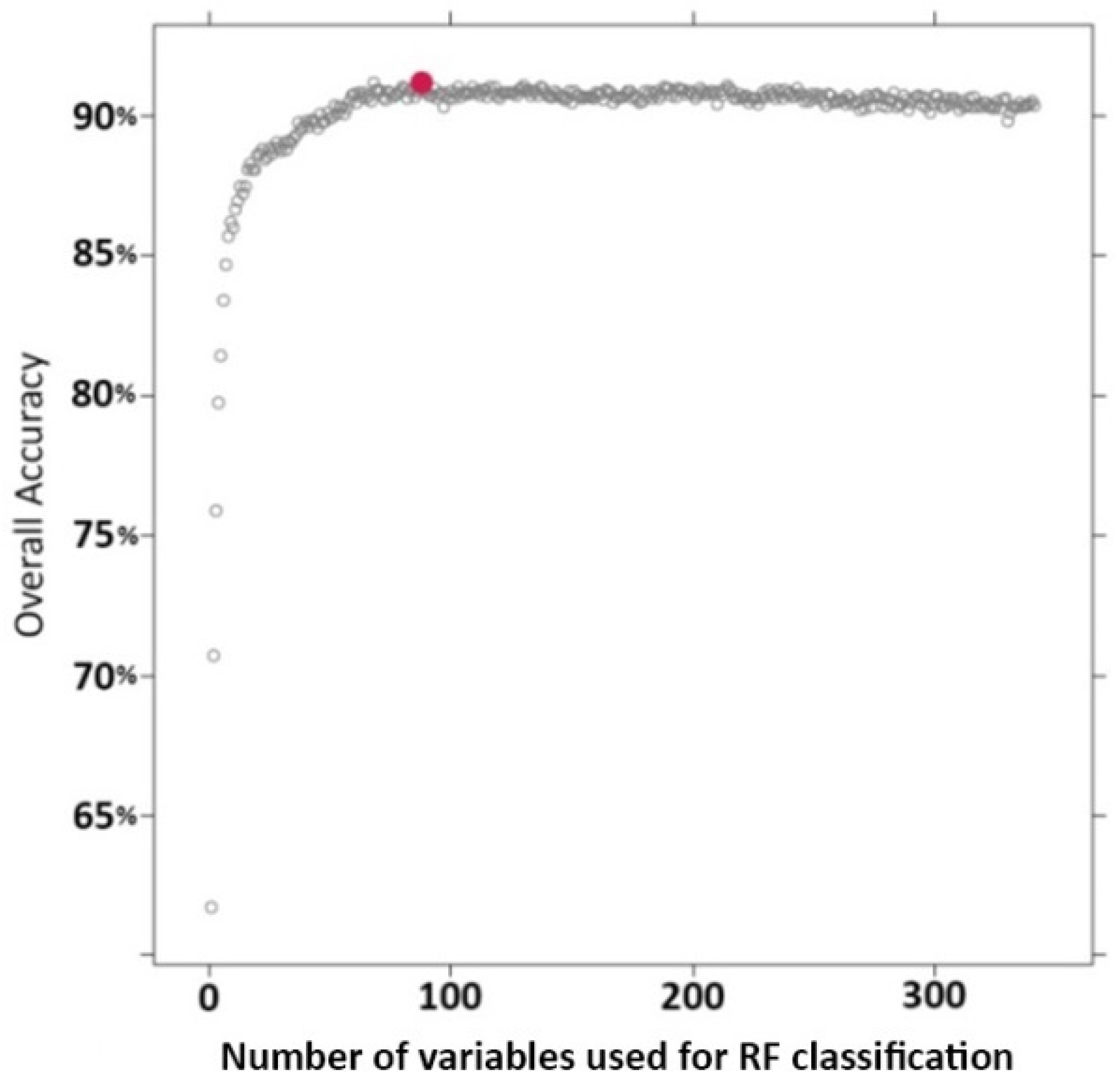
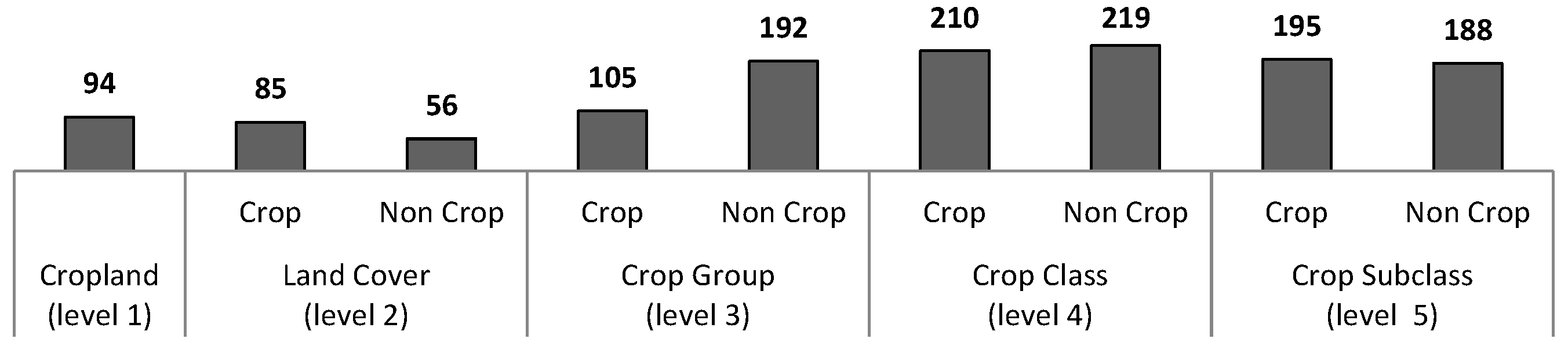
We first optimized the classifier by reducing the number of features to be extracted for an implementation facility. The results of the optimization phase show that the number of features to be extracted before applying the optimized classifiers to an entire study zone could be significantly reduced from 1.5- to 6-fold, depending on the nomenclature level, with no significant effects on classification accuracy. This could lead to significant gains in computation time for generating object features given that, for the 60 km × 60 km site, the segmentation process for the whole area produced more than 6 million objects for which features must be extracted.

With this classification scheme, the first level of the nomenclature (cropland) was classified very well (OA of 91.7%). The “crop” class was better classified than the “non-crop” class (f1-scores of 0.93 and 0.89, respectively) due to the relative homogeneity of the “crop” class (only composed of crops) compared to the heterogeneity of the “non-crop” class (composed of forests, water bodies, built-up surfaces, etc.).

The hierarchical approach (first isolating “crop” and “non-crop” domains at level 1, then performing classifications within each domain at following nomenclature levels) improved significantly the accuracy of the classifications for the majority of classes from levels 2 (land cover) to 5 (crop subclass) when compared to the classical approach. However, as expected, rainfed crops were difficult to classify even for major crops such as “maize” and “rainfed rice” (f1-scores of 0.61 and 0.65 at level 5, respectively). This can be attributed to the very small size (often lower than the size of one or two 10 m pixels) of cropped objects within the rainfed area, precluding a pure crop signal at the Sentinel-2 spatial resolution. The configuration of the rainfed cultivated domain composed of a patchwork of small agricultural fields and natural vegetation patches and the frequent practice of mixed cropping also complicated the correct classification of rainfed crops. The presence of mixed pixels in the HRS time series did not affect the classification of cropland (level 1 of the nomenclature) for which accuracy was good, as expected by the study of [9] which showed that a 10 m spatial resolution was adapted for cropland classification, even in the typical fragmented landscapes of smallholder agricultural areas. However, it seemed to be a major source of error in the classification of more detailed levels (crop group, crop type, crop subclass). The same limits can be observed on more intensive agriculture, for crop type classification of large and regular shaped fields with LSR sensors [46], as the likelihood of finding mixed pixels is a function of the spatial resolution of the image, the thematic detail to be mapped, and the size and spatial pattern of land cover patches [47].

By contrast, the classification scheme was shown to be accurate at classifying crops within the irrigated domain, as only irrigated rice occupied this area, resulting in larger patches of the same crop with a specific spectral response due to the presence of a surface water layer. Consequently, “irrigated rice” was classified with a high f1-score of 0.82, allowing for classification of this key crop in terms of food security, with a high level of confidence. All of these results should, however, be interpreted with in mind the fact that the training set represented only 0.038% of the total number of objects in the study area (more the 6 million), whereas studies like [48] recommend a training set of 0.25% of the whole study area, meaning more than 15,000 training samples in our case. Such maps could be validated according to the method provided by [49] for area-based and location-based validation of the classified images using OBIA, in order to spatially identify where there is error or uncertainty.

In terms of performance, it is very difficult to compare our results with those of previous studies or even with those of studies performed in the same area or with equivalent agricultural systems since satellite time series (with key dates of data acquisition), ground truth data, and/or nomenclature are rarely the same. For instance, [22] performed classifications of major crop types of the same site in Madagascar based only on HSR time series (mainly from SPOT4 Take5 experiments), and an RF classifier applied at the pixel level to a reduced set of variables (reflectances and three spectral indices) within a cropland mask. While the authors achieved a classification accuracy of 50.2% for the discrimination of four main crops, we achieved a value of 64.1% at an equivalent nomenclature level for the discrimination of 14 crop classes. As noted above, simple comparisons should be made only with caution.

4.2. Recommendations and Outlooks for the Operational Mapping of Smallholder Agricultural Systems

In our approach, features were extracted from satellite images to build the learning database based on the following assumptions: (i) crops’ spectral and temporal behaviors can be captured through a set of attributes extracted from time series of multispectral images; (ii) the boundaries of structuring objects in a landscape and inside object heterogeneity (texture) can be extracted from VHSR data; and (iii) ancillary environmental data such as the topography extracted from a DEM can be used to discriminate between different land use types in constrained environments (e.g., water available for irrigation in lowlands).

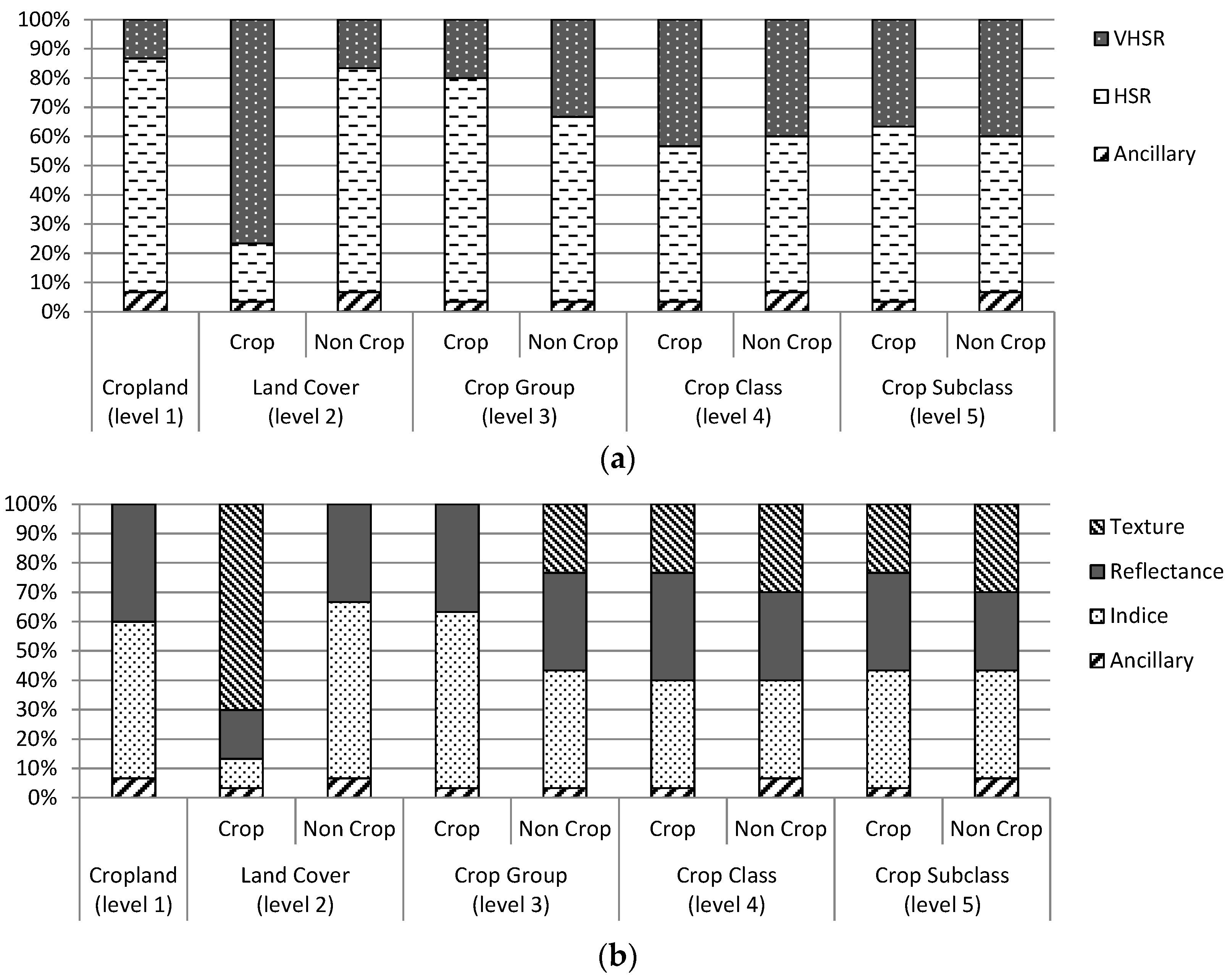
The analysis of the sources of important variables, which were ranked using the MDA measure, showed that the variables derived from the HSR time series were much more informative than the variables derived from VHSR or ancillary data (with the exception of the “ligneous crop”/“annual crop” discrimination, which clearly benefits from the VHSR textural indices). When focusing on types of variables, spectral indices were shown to be the more relevant variables, followed closely by reflectances. This was confirmed through our analysis of the contributions of the different variables to classification accuracy, which showed that eliminating VHSR spectral, textural or ancillary data did not significantly impact the classification results and that spectral indices extracted from the HSR time series were the most discriminant. These results were obtained from an unbalanced small training set, and some studies warn of discrepancies that can be observed in variable importance for such sampling designs [50]. Despite this fact, our results are consistent with the conclusions of [27], who used OBIA and decision trees for crop identification with ASTER (Advanced Spaceborne Thermal Emission and Reflection Radiometer) data and showed that textural indices are secondary variables. In conclusion, in this approach, VHSR data are critical for segmentation but are not necessary for classification. In light of this, considerable gains in computation time can be achieved by eliminating VHSR texture calculation and feature extraction tasks.

In this experiment, we also analyzed the performances of our classification approach at different levels of nomenclature, from cropland (two classes) to crop subclass (25 classes). Not surprisingly, the more complex the nomenclature was, the less performing was the approach, especially for classes belonging to cropland. This allowed for identifying the land uses that could be classified with an acceptable accuracy (≥75%) at each nomenclature level. Inside cropland, important crop groups (cereals, fruit crops) and types (rice, fodder crops) were well classified with a class accuracy level above 75%, while for other minor crops, such as leguminous, vegetable, root and tuber crops, accuracy levels between 50% and 60% were achieved. For rice, the dominant crop in the area, our classification approach allowed us to separate rainfed areas from irrigated areas with 82% accuracy (for irrigated rice).

Our results also showed that even when the spatial resolution of a time series is too coarse to obtain a pure signal, temporal information is essential for characterization and discrimination of land uses in such complex small-scale agricultural areas. Improvements in classification accuracy could also be achieved by accounting for the chronology of the time series in Random Forest through the calculation of new variables linked to the phenology, as proposed in [51,52] for the MODIS time series, even though [51] found that phenological variables are less important than reflectances or spectral indices.

Finally, we are aware that the quality of classifications can fluctuate depending on the number and period of clear image acquisition dates. However, the upcoming availability of Sentinel-2 data with a five-day acquisition frequency is expected to improve the probability of obtaining clear images in such tropical and cloudy environments.

5. Conclusions

This paper presents an in-depth study on the use of multisource data for classifying tropical smallholder agriculture at different nomenclature levels using a combined OBIA–Random Forest classification scheme. Our results show that, even for smallholder agricultural systems, maps separating cropland from non-cropland can be produced from a high spatial resolution time series and a very high spatial resolution image with an overall accuracy level above 90% and can be made available for agricultural public policy makers. This type of information is particularly essential for countries that are frequently affected by food crises and where information on acreage and locations of cultivated areas are sorely lacking.

Concerning the characterization of the land use inside the cropland, the major crop group (cereals) and crop type (rice) of the study area were classified well with a class accuracy level close to 80%. For rice, the dominant crop in the area, our classification approach allowed us to separate rainfed areas from irrigated areas with 82% accuracy (for irrigated rice). This information is particularly useful for food security monitoring, as irrigated systems are more productive than rainfed ones, and their relative proportions impact food supply forecasting.

Regarding the availability of data for applying this approach to larger areas, Sentinel-2 time series are now provided on a 10-day basis and will soon be available every five days for the whole country at no charge. This gain in acquisition frequency is particularly important in tropical cloudy areas and is expected to help improving crop classification accuracy thanks to a better description of crop growth. Very high spatial resolution images that are essential in this approach for segmentation of the area into objects remain costly to acquire annually at a regional scale. However, recent initiatives promoting nanosatellites (e.g., Planet^®) announce the availability of very high spatial resolution images, with high revisit frequency at reasonable cost.

References

1. Thornton, P. Mapping Poverty and Livestock in the Developing World; International Livestock Research Institute (aka ILCA and ILRAD): Nairobi, Kenya, 2002; Volume 1. [Google Scholar]
2. Morton, J.F. The impact of climate change on smallholder and subsistence agriculture. Proc. Natl. Acad. Sci. USA 2007, 104, 19680–19685. [Google Scholar] [CrossRef] [PubMed]
3. Biradar, C.M.; Xiao, X. Quantifying the area and spatial distribution of double-and triple-cropping croplands in India with multi-temporal modis imagery in 2005. Int. J. Remote Sens. 2011, 32, 367–386. [Google Scholar] [CrossRef]
4. Ozdogan, M. The spatial distribution of crop types from MODIS data: Temporal unmixing using independent component analysis. Remote Sens. Environ. 2010, 114, 1190–1204. [Google Scholar] [CrossRef]
5. Qiu, J.; Tang, H.; Frolking, S.; Boles, S.; Li, C.; Xiao, X.; Liu, J.; Zhuang, Y.; Qin, X. Mapping single-, double-, and triple-crop agriculture in china at 0.5° × 0.5° by combining country-scale census data with a remote sensing derived land cover map. Geocarto Int. 2003, 18, 3–13. [Google Scholar] [CrossRef]
6. Xiao, X.; Boles, S.; Liu, J.; Zhuang, D.; Frolking, S.; Li, C.; Salas, W.; Moore, B. Mapping paddy rice agriculture in southern China using multi-temporal MODIS images. Remote Sens. Environ. 2005, 95, 480–492. [Google Scholar] [CrossRef]
7. Zhang, X.; Friedl, M.; Schaaf, C. Sensitivity of vegetation phenology detection to the temporal resolution of satellite data. Int. J. Remote Sens. 2009, 30, 2061–2074. [Google Scholar] [CrossRef]
8. Boschetti, L.; Flasse, S.P.; Brivio, P.A. Analysis of the conflict between omission and commission in low spatial resolution dichotomic thematic products: The pareto boundary. Remote Sens. Environ. 2004, 91, 280–292. [Google Scholar] [CrossRef]
9. Leroux, L.; Jolivot, A.; Bégué, A.; Lo Seen, D.; Zoungrana, B. How reliable is the MODIS land cover product for crop mapping sub-saharan agricultural landscapes? Remote Sens. 2014, 6, 8541–8564. [Google Scholar] [CrossRef] [Green Version]
10. Drusch, M.; Del Bello, U.; Carlier, S.; Colin, O.; Fernandez, V.; Gascon, F.; Hoersch, B.; Isola, C.; Laberinti, P.; Martimort, P. Sentinel-2: ESA’s optical high-resolution mission for GMES operational services. Remote Sens. Environ. 2012, 120, 25–36. [Google Scholar] [CrossRef]
11. Zhou, F.; Zhang, A.; Townley-Smith, L. A data mining approach for evaluation of optimal time-series of MODIS data for land cover mapping at a regional level. ISPRS J. Photogramm. Remote Sens. 2013, 84, 114–129. [Google Scholar] [CrossRef]
12. Rodriguez-Galiano, V.F.; Ghimire, B.; Rogan, J.; Chica-Olmo, M.; Rigol-Sanchez, J.P. An assessment of the effectiveness of a random forest classifier for land-cover classification. ISPRS J. Photogramm. Remote Sens. 2012, 67, 93–104. [Google Scholar] [CrossRef]
13. Breiman, L. Random forests. Mach. Learn. 2001, 45, 5–32. [Google Scholar] [CrossRef]
14. Chan, J.C.-W.; Paelinckx, D. Evaluation of random forest and adaboost tree-based ensemble classification and spectral band selection for ecotope mapping using airborne hyperspectral imagery. Remote Sens. Environ. 2008, 112, 2999–3011. [Google Scholar] [CrossRef]
15. Debats, S.R.; Luob, D.; Estes, L.D.; Fuchs, T.J.; Caylor, K. A generalized computer vision approach to mapping crop fields in heterogeneous agricultural landscapes. Remote Sens. Environ. 2016, 179, 210–221. [Google Scholar] [CrossRef]
16. Ghimire, B.; Rogan, J.; Miller, J. Contextual land-cover classification: Incorporating spatial dependence in land-cover classification models using random forests and the Getis statistic. Remote Sens. Lett. 2010, 1, 45–54. [Google Scholar] [CrossRef]
17. Lawrence, R.L.; Wood, S.D.; Sheley, R.L. Mapping invasive plants using hyperspectral imagery and breiman cutler classifications (randomforest). Remote Sens. Environ. 2006, 100, 356–362. [Google Scholar] [CrossRef]
18. Pal, M. Random forest classifier for remote sensing classification. Int. J. Remote Sens. 2005, 26, 217–222. [Google Scholar] [CrossRef]
19. Pringle, M.J.; Denham, R.J.; Devadas, R. Identification of cropping activity in central and southern queensland, australia, with the aid of MODIS MOD13Q1 imagery. Int. J. Appl. Earth Obs. Geoinf. 2012, 19, 276–285. [Google Scholar] [CrossRef]
20. Sesnie, S.E.; Gessler, P.E.; Finegan, B.; Thessler, S. Integrating Landsat TM and SRTM-DEM derived variables with decision trees for habitat classification and change detection in complex neotropical environments. Remote Sens. Environ. 2008, 112, 2145–2159. [Google Scholar] [CrossRef]
21. Bontemps, S.; Arias, M.; Cara, C.; Dedieu, G.; Guzzonato, E.; Hagolle, O.; Inglada, J.; Matton, N.; Morin, D.; Popescu, R.; et al. Building a sentinel-2 like data set specifically dedicated to agriculture monitoring over 12 sites globally distributed. Remote Sens. 2015, 7, 16062–16090. [Google Scholar] [CrossRef]
22. Inglada, J.; Arias, M.; Tardy, B.; Hagolle, O.; Valero, S.; Morin, D.; Dedieu, G.; Sepulcre, G.; Bontemps, S.; Defourny, P.; et al. Assessment of an operational system for crop type map production using high temporal and spatial resolution satellite optical imagery. Remote Sens. 2015, 7, 12356–12379. [Google Scholar] [CrossRef]
23. Theia Land Data Centre. Available online: https://www.theia-land.fr/en/products/spot4-take5 (accessed on 18 September 2015).
24. Vaudour, E.; Noirot-Cosson, P.; Membrive, O. Early-season mapping of crops and cultural operations using very high spatial resolution pléiades images. Int. J. Appl. Earth Obs. Geoinf. 2015, 42, 128–141. [Google Scholar] [CrossRef]
25. Chehata, N.; Ghariani, K.; Le Bris, A.; Lagacherie, P. Délimitation des parcelles agricoles par classification d’images pléiades. Rev. Fr. Photogramm. Teledetec. 2015, 209, 165–171. [Google Scholar]
26. Blaschke, T.; Hay, G.J.; Kelly, M.; Lang, S.; Hofmann, P.; Addink, E.; Feitosa, R.Q.; van der Meer, F.; van der Werff, H.; van Coillie, F. Geographic object-based image analysis–towards a new paradigm. ISPRS J. Photogramm. Remote Sens. 2014, 87, 180–191. [Google Scholar] [CrossRef] [PubMed]
27. Peña-Barragán, J.M.; Ngugi, M.K.; Plant, R.E.; Six, J. Object-based crop identification using multiple vegetation indices, textural features and crop phenology. Remote Sens. Environ. 2011, 115, 1301–1316. [Google Scholar] [CrossRef]
28. Castillejo-González, I.L.; López-Granados, F.; García-Ferrer, A.; Peña-Barragán, J.M.; Jurado-Expósito, M.; de la Orden, M.S.; González-Audicana, M. Object-and pixel-based analysis for mapping crops and their agro-environmental associated measures using quickbird imagery. Comput. Electron. Agric. 2009, 68, 207–215. [Google Scholar] [CrossRef]
29. Ursani, A.A.; Kpalma, K.; Lelong, C.; Ronsin, J. Fusion of textural and spectral information for tree crop and other agricultural cover mapping with very-high resolution satellite images. IEEE J. Sel. Top. Appl. Earth Obs. Remote Sens. 2012, 5, 225–235. [Google Scholar] [CrossRef]
30. Li, M.; Ma, L.; Blaschke, T.; Cheng, L.; Tiede, D. A systematic comparison of different object-based classification techniques using high spatial resolution imagery in agricultural environments. Int. J. Appl. Earth Obs. Geoinf. 2016, 49, 87–98. [Google Scholar] [CrossRef]
31. Laben, C.A.; Brower, B.V. Process for Enhancing the Spatial Resolution of Multispectral Imagery Using Pan-Sharpening. U.S. Patent No. 6,011,875, 4 January 2000. [Google Scholar]
32. OTB-Team. Orfeo Toolbox. Available online: Http://www.Orfeo-toolbox.Org/ (accessed on 18 September 2015).
33. Baatz, M.; Schäpe, A. Multiresolution segmentation: An optimization approach for high quality multi-scale image segmentation. Angew. Geogr. Informationsverarbeitung XII 2000, 58, 12–23. [Google Scholar]
34. Trimble. Ecognition Developer 9.0 Reference Book; Trimble Germany: Munich, Germany, 2014. [Google Scholar]
35. Rouse, J.W., Jr.; Haas, R.; Schell, J.; Deering, D. Monitoring vegetation systems in the great plains with ERTS. NASA Spec. Publ. 1974, 351, 309. [Google Scholar]
36. Gao, B.C. Ndwi—A normalized difference water index for remote sensing of vegetation liquid water from space. Remote Sens. Environ. 1996, 58, 257–266. [Google Scholar] [CrossRef]
37. Xu, H. Modification of normalised difference water index (NDWI) to enhance open water features in remotely sensed imagery. Int. J. Remote Sens. 2006, 27, 3025–3033. [Google Scholar] [CrossRef]
38. Haralick, R.M.; Shanmugam, K. Textural features for image classification. IEEE Trans. Syst. Man Cybern. 1973, SMC-3, 610–621. [Google Scholar] [CrossRef]
39. Cutler, D.R.; Edwards, T.C.; Beard, K.H.; Cutler, A.; Hess, K.T.; Gibson, J.; Lawler, J.J. Random forests for classification in ecology. Ecology 2007, 88, 2783–2792. [Google Scholar] [CrossRef] [PubMed]
40. Liaw, A.; Wiener, M. Classification and regression by randomforest. R News 2002, 2, 18–22. [Google Scholar]
41. R Development Core Team. R: A Language and Environment for Statistical Computing; R Foundation for Statistical Computing, R Foundation for Statistical Computing: Vienna, Austria; Available online: http://www.R-project.org (accessed on 15 November 2016).
42. Max Kuhn. Contributions from Jed Wing, S.W., Andre Williams, Chris Keefer and Allan Engelhardt, Caret: Classification and Regression Training, R Package Version 5.15-044. Available online: http://cran.R-project.Org/package=caret (accessed on 15 November 2016).
43. Cohen, J. A coefficient of agreement for nominal scales. Educ. Psychol. Meas. 1960, 20, 37–46. [Google Scholar] [CrossRef]
44. Rosenfield, G.H.; Fitzpatrick-Lins, K. A coefficient of agreement as a measure of thematic classification accuracy. Photogramm. Eng. Remote Sens. 1986, 52, 223–227. [Google Scholar]
45. McNemar, Q. Note on the sampling error of the difference between correlated proportions or percentages. Psychometrika 1947, 12, 153–157. [Google Scholar] [CrossRef]
46. Löw, F.; Duveiller, G. Defining the spatial resolution requirements for crop identification using optical remote sensing. Remote Sens. 2014, 6, 9034–9063. [Google Scholar] [CrossRef]
47. Moody, A.; Woodcock, C.E. Scale-dependent errors in the estimation of land-cover proportions. Implications for global land-cover datasets. Photogramm. Eng. Remote Sens. 1994, 60, 585–596. [Google Scholar]
48. Colditz, R.R. An evaluation of different training sample allocation schemes for discrete and continuous land cover classification using decision tree-based algorithms. Remote Sens. 2015, 7, 9655–9681. [Google Scholar] [CrossRef]
49. Whiteside, T.G.; Maier, S.W.; Boggs, G.S. Area-based and location-based validation of classified image objects. Int. J. Appl. Earth Obs. Geoinf. 2014, 28, 117–130. [Google Scholar] [CrossRef]
50. Janitza, S.; Strobl, C.; Boulesteix, A.-L. An auc-based permutation variable importance measure for random forests. BMC Bioinform. 2013, 14, 119. [Google Scholar] [CrossRef] [PubMed] [Green Version]
51. Hao, P.; Zhan, Y.; Wang, L.; Niu, Z.; Shakir, M. Feature selection of time series MODIS data for early crop classification using random forest: A case study in kansas, USA. Remote Sens. 2015, 7, 5347–5369. [Google Scholar] [CrossRef]
52. Senf, C.; Hostert, P.; van der Linden, S. Using MODIS time series and random forests classification for mapping land use in south-east Asia. In Proceedings of the 2012 IEEE International Geoscience and Remote Sensing Symposium (IGARSS), Munich, Germany, 22–27 July 2012; pp. 6733–6736.
Figure 1. (a) location of collected waypoints in the study area (background image: Landsat 8 acquired on 15 June 2015) and (b) ground polygon samples (background image: PLEIADES acquired on 14 February 2015).
Remotesensing 09 00259 g001
Figure 2. Chronogram of the 2014–2015 satellite acquisitions. The cloud percentage represents the proportion of clouds over polygons of the ground database for each acquisition date. For the PLEIADES coverage, 16th March 2015 (D15 for date 15 of the time series) was chosen to represent the median acquisition date of the different tiles.
Remotesensing 09 00259 g002
Figure 3. Evolution of cross-validated (5-fold) overall accuracy according to the number of variables used for classification at level 1 (cropland). The variables were previously ranked by order of importance based on the MDA measure.
Remotesensing 09 00259 g003
Figure 4. Optimal number of variables needed to reach the best level of overall accuracy for each domain (crop/non-crop) and each nomenclature level via a hierarchical approach.
Remotesensing 09 00259 g004
Figure 5. Maps obtained at level 1, cropland (a), and level 5, crop subclass (b), via the hierarchical classification approach.
Remotesensing 09 00259 g005
Figure 6. Proportions of different sources— high spatial resolution imagery (HSR), very high spatial resolution imagery (VHSR), and ancillary—(a) and types—reflectances, spectral indices, textures, and ancillary—(b) of variables among the 30 most important variables (ranked by MDA measure) for each level of the JECAM (Joint Experiment for Crop Assessment and Monitoring) nomenclature.
Remotesensing 09 00259 g006