Estimation of Pine Forest Height and Underlying DEM Using Multi-Baseline P-Band PolInSAR Data

Abstract

On the basis of the Gaussian vertical backscatter (GVB) model, this paper proposes a new method for extracting pine forest height and forest underlying digital elevation model (FUDEM) from multi-baseline (MB) P-band polarimetric-interferometric radar (PolInSAR) data. Considering the linear ground-to-volume relationship, the GVB is linked to the interferometric coherences of different polarizations. Subsequently, an inversion algorithm, weighted complex least squares adjustment (WCLSA), is formulated, including the mathematical model, the stochastic model and the parameter estimation method. The WCLSA method can take full advantage of the redundant observations, adjust the contributions of different observations and avoid null ground-to-volume ratio (GVR) assumption. The simulated experiment demonstrates that the WCLSA method is feasible to estimate the pure ground and volume scattering contributions. Finally, the WCLSA method is applied to E-SAR P-band data acquired over Krycklan Catchment covered with mixed pine forest. It is shown that the FUDEM highly agrees with those derived by LiDAR, with a root mean square error (RMSE) of 3.45 m, improved by 23.0% in comparison to the three-stage method. The difference between the extracted forest height and LiDAR forest height is assessed with a RMSE of 1.45 m, improved by 37.5% and 26.0%, respectively, for model and inversion aspects in comparison to three-stage inversion based on random volume over ground (RVoG) model.

1. Introduction

Polarimetric-interferometric radar (PolInSAR) provides a promising remote sensing technique for estimating forest height and ground phase by its sensitivity to the forest vertical structure [1,2,3,4]. The complex interferometric coherence has been related to the vertical distribution of the forest scatterers [2,3,4]. Consequently, PolInSAR presents the capacity to measure ground and volume scattering contributions, which leads to the possibility of extracting the forest underlying digital elevation model (FUDEM) and forest height [1,2,3,4,5,6,7,8]. Both of them are critical to the digital forest management.

Generally, the inversions of FUDEM and forest height are performed with the random volume over ground (RVoG) model, with the assumption that the vegetation layer is a vertical homogeneous volume with a constant extinction [4]. This assumption is adapted to the forest height inversion at high frequencies (e.g., X-, C- and L-band) since the main scatterers are leaves and twigs [8,9,10]. However, at low frequencies (e.g., P-band), the radar wave interacts with the large-scale forest structural elements (e.g., branches and trunks) in the whole forest height extent [11]. In this situation, the forest vertical heterogeneity should be considered and integrated in the forest scattering models. To cope with this problem, Garestier et al. [11,12] proposed the Gaussian vertical backscatter (GVB) model, which can depict the forest vertical heterogeneity by describing the predominant contribution of volume scattering located in a finite height.

The GVB model is very complicated since it captures complex natural features of the forest, which results in the impossibility to invert the forest parameters from single baseline (SB) PolInSAR without using external data like forest underlying terrain and forest height or the vertical structure information of the forest [11,12]. However, these external data are very difficult to collect in practice. In addition, in order to obtain the pure volume scattering contribution, it should assume that there is at least one polarization channel without ground scattering contribution (null GVR assumption) as demonstrated in the three-stage method [13]. However, this is impossible at P band because the volume and ground scattering contributions are always mixed in all the polarization channels due to the large penetration depth [14,15]. Previous works [16,17,18,19,20] have demonstrated that the multi-baseline (MB) increases observation space, which allows estimating forest height and ground phase from the forest scattering model directly without external data or priori information. However, the MB PolInSAR inversion framework usually presents a high complexity due to the nonlinear nature of the scattering model. Hence, intelligent optimizations or multi-step methods are usually adopted to ease the inversion. However, these methods on one hand have difficulties in taking full advantage of the redundant observations which can enhance the robustness of the estimation, and on the other hand are incapable to adjust the contributions of the interferometric coherence values perturbed by different levels of noise to the solutions.

The aim of this work is to cope with such limitations and extract accurate forest height and FUDEM from MB PolInSAR data. The GVB model is adopted since it can account for forest vertical heterogeneity at P band. Next, a mathematical model on the basis of GVB is developed in order to combine all available observations of the MB PolInSAR and accurately separate the pure ground and volume scattering contributions from the total PolInSAR signal. Then, a stochastic model based on the Cramer–Rao bound [1,21] on variance of coherence is proposed, aiming at describing the contributions of the interferometric coherence values to the solutions. In addition, an inversion algorithm, weighted complex least squares adjustment, integrating the above mentioned mathematical function and stochastic model, is proposed in order to suppress the errors in the observations and improve the accuracy of the solutions. Finally, the FUDEM and forest height can be respectively extracted with the estimated pure ground and volume scattering contributions.

This paper is structured as follows. The principle of the GVB model is introduced and discussed in Section 2. Section 3 presents the weighted complex least squares adjustment (WCLSA) methodology for the GVB inversion, including the mathematical model, the stochastic model, the parameter estimation and an extraction of the FUDEM and forest height. The retrievals of the FUDEM and forest height are presented in Section 4. Finally, the conclusions are drawn in Section 5.

2. Description of Forest Vertical Structure with GVB

2.1. GVB Model

The GVB describes the forest area as a two-layer model, the vegetation layer and the ground layer [11,12]. The Gaussian function is employed to depict the vertical heterogeneity of the vegetation layer given the fact that for most forest types the matter density is much higher at the lower part than the top of the canopy [11,22]. In detail, the forest vertical structure function can be entirely defined by three parameters: forest height h_v and two Gaussian function parameters $\delta$ and $\chi$. Then, the interferometric coherence of volume layer can be expressed as [11]

$${\gamma }_v\left(h_v,\delta ,\chi \right)=\frac{{\displaystyle {\int }_0^{h_v}{e}^{-\frac{{\left(z-\delta \right)}^2}{2{\chi }^2}+j{k}_{z}z}dz}}{{\displaystyle {\int }_0^{h_v}{e}^{-\frac{{\left(z-\delta \right)}^2}{2{\chi }^2}}dz}}$$

(1)

where $\delta$ is the elevation of the strongest backscatter power. $\chi$ represents the corresponding standard deviation (std). j is the imagery unit. z is the variable of integration which ranges from 0 to h_v. k_z is the vertical wavenumber and can be expressed as [1]

$$k_z=\frac{4\pi }{\lambda \sin \theta }\Delta \theta$$

(2)

where $\theta$ is the incidence angle and $\Delta \theta$ denotes the incidence angle difference between master and slave images. Combined with the Gaussian error function erf, the integrals of Equation (1) can be expressed as

$${\gamma }_v\left(h_v,\delta ,\chi \right)=e^{-\frac{{\chi }^2{k}_z^2}{2}+j\delta k_z}\frac{erf\left(\frac{1}{\sqrt{2}}\left(j\chi k_z+\frac{\delta }{\chi }\right)\right)-erf\left(\frac{1}{\sqrt{2}}\left(j\chi k_z+\frac{\delta -h_v}{\chi }\right)\right)}{erf\left(\frac{h_v-\delta }{\sqrt{2}\chi }\right)+erf\left(\frac{\delta }{\sqrt{2}\chi }\right)}$$

(3)

Next, the volume layer is coupled with the ground layer and the GVB can be expressed as [11]

$$\gamma (\omega )=e^{i{\phi }_0}\frac{{\gamma }_v\left(h_v,\delta ,\chi \right)+\mu (\omega )}{1+\mu (\omega )}$$

(4)

where $\gamma (\omega )$ is the complex interferometric coherence. $\omega$ is the polarization state vector. ${\phi }_0$ denotes the ground phase which can be used to estimate the FUDEM. $\mu$ is the polarization-dependent GVR.

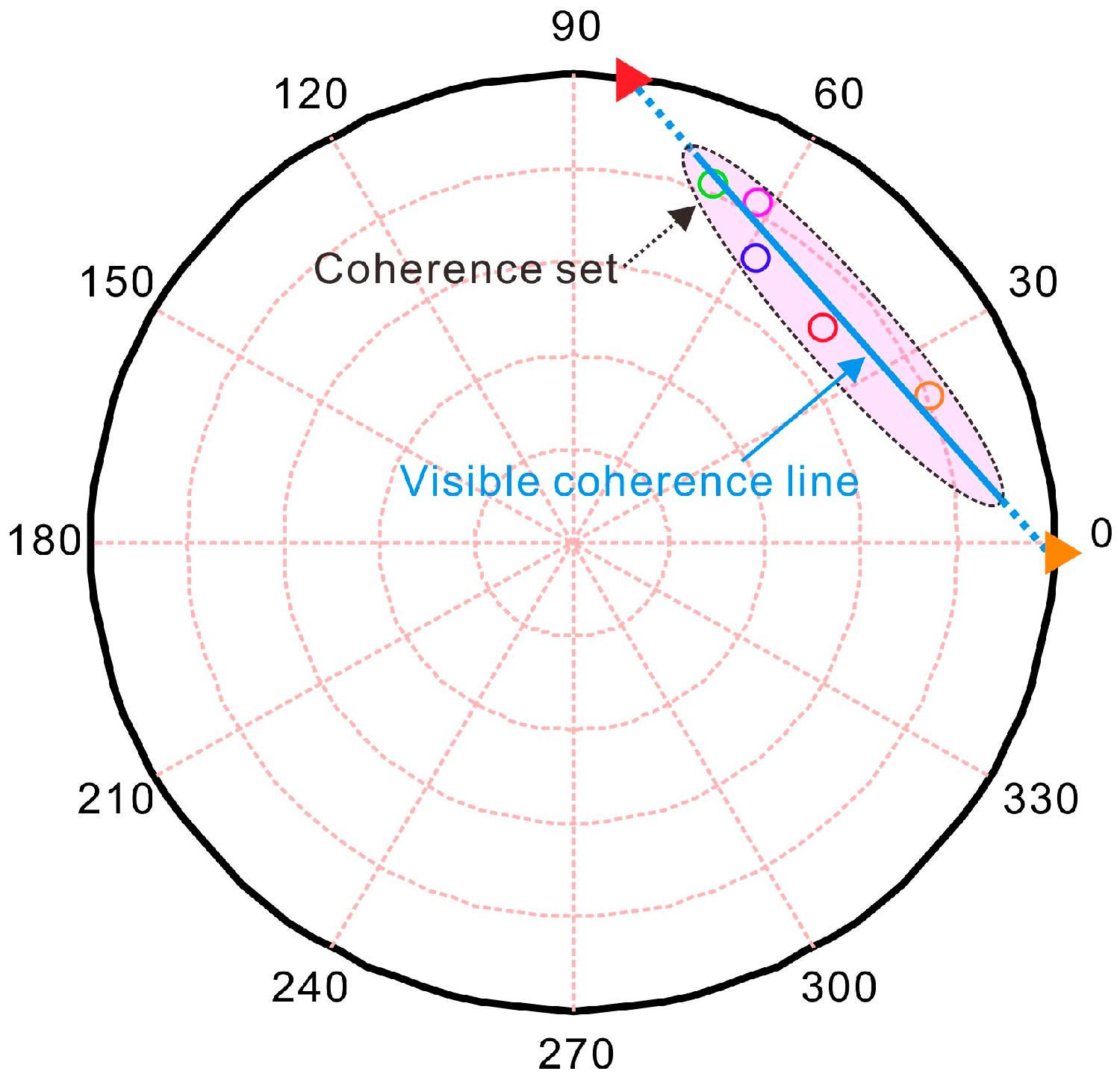
2.2. Coherence Locus of GVB

At P band, precious works have shown that the volume scattering contribution is polarization-dependent since the orientation effect has been observed over forests [14,15,23]. As a result, this cannot meet the RVoG assumption and may induce biases of ground phase estimated by the three-stage inversion procedure [23]. Nonetheless, the biases may be small and acceptable forest height results have been successfully extracted using the RVoG assumption at P band over the tropical and pine forests [24,25,26,27]. Hence, in this paper, the volume scattering contribution is still assumed to be polarization-independent for the GVB model. In this way, the GVB is clearly linear with respect to the GVR. Thus, coherences associated with different polarizations are located on a line in the complex plane. However, they are not located on a line in practice due to the influence of noise as displayed in Figure 1. Therefore, a line fitting technique can be used to reconstruct the coherence line from the noisy coherences [13]. Then the ground phase can be identified from the intersections between the coherence line and the complex unit circle in terms of rank order of the coherence values [13].

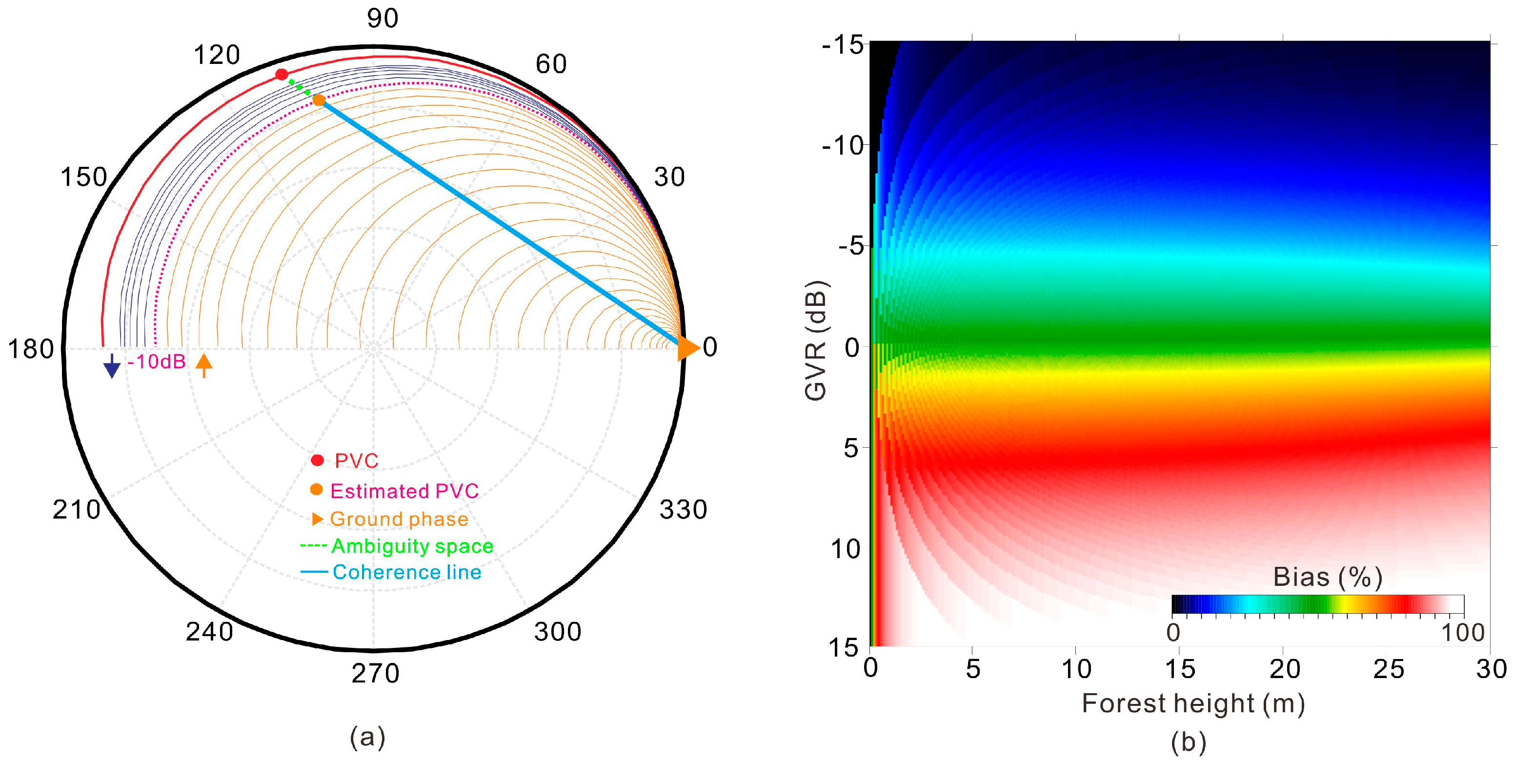
2.3. Discussion of Null GVR Assumption

In order to measure the pure volume scattering contribution from SB PolInSAR data, a null GVR is always done [11]. Thus, Equation (4) can be converted into

$$\gamma (\omega )=e^{i{\phi }_0}{\gamma }_v\left(h_v,\delta ,\chi \right)$$

(5)

The assumption of null GVR gives rise to a ambiguity space when we calculate the pure volume coherence (PVC), especially for low frequency PolInSAR data or high frequency PolInSAR data over a sparse forest region, because volume and ground scattering contributions are mixed in all the polarization channels.

To illustrate the sensitivity of forest height to the GVR in the complex plane, a simulated experiment is conducted with Equation (4). Forest heights ranging from 0 to 30 m are combined with $\delta$ of h_v/4 and $\chi$ of h_v/12. k_z is set 0.209. The simulated interferometric coherences under the null GVR condition are presented in the complex plane as the red line shown in Figure 2a. After that, the GVR goes from −15 to 15 dB and the corresponding interferometric coherences are superposed on the common complex plane as shown in the figure. The blue lines represent interferometric coherences associated with the GVR that is smaller than −10 dB (the pink line) and the yellow lines represent interferometric coherences corresponding to the GVR that is larger than −10 dB. We can see the corresponding coherence sets shrink to the ground phase point gradually as the GVR increases, and larger ambiguity space (the green dashed line) appears if the null GVR assumption is still done. The shrinking of the coherence sets leads to the fluctuation of the PVC magnitude, but only decrease of the PVC phase. Figure 2b is a quantitative analysis about the bias of the forest height under the assumption of null GVR. Assuming $\delta$ and $\chi$ are known, the height is calculated with Equation (5). Simulation results show that there is a 10% underestimation of the forest height when the GVR is less than −10 dB. We also can observe that the bias significantly increases with the GVR. For example, the bias can be up to about 50% when the GVR is up to 0 dB. Furthermore, the inversion of forest height almost fails if the GVR is larger than 0 dB. Therefore, for estimating a height accuracy of 10%, the GVR of one polarization should be smaller than −10 dB.

3. Parameter Inversion Based on Weighted Complex Least Squares

In this section, we introduce a novel inversion framework for the GVB on the basis of the WCLSA in the MB PolInSAR configuration, in order to design a robust methodology to estimate the pure ground and volume scattering contributions without external data and null GVR assumption. Then, the FUDEM and forest height can be extracted with the obtained pure ground and volume scattering contributions.

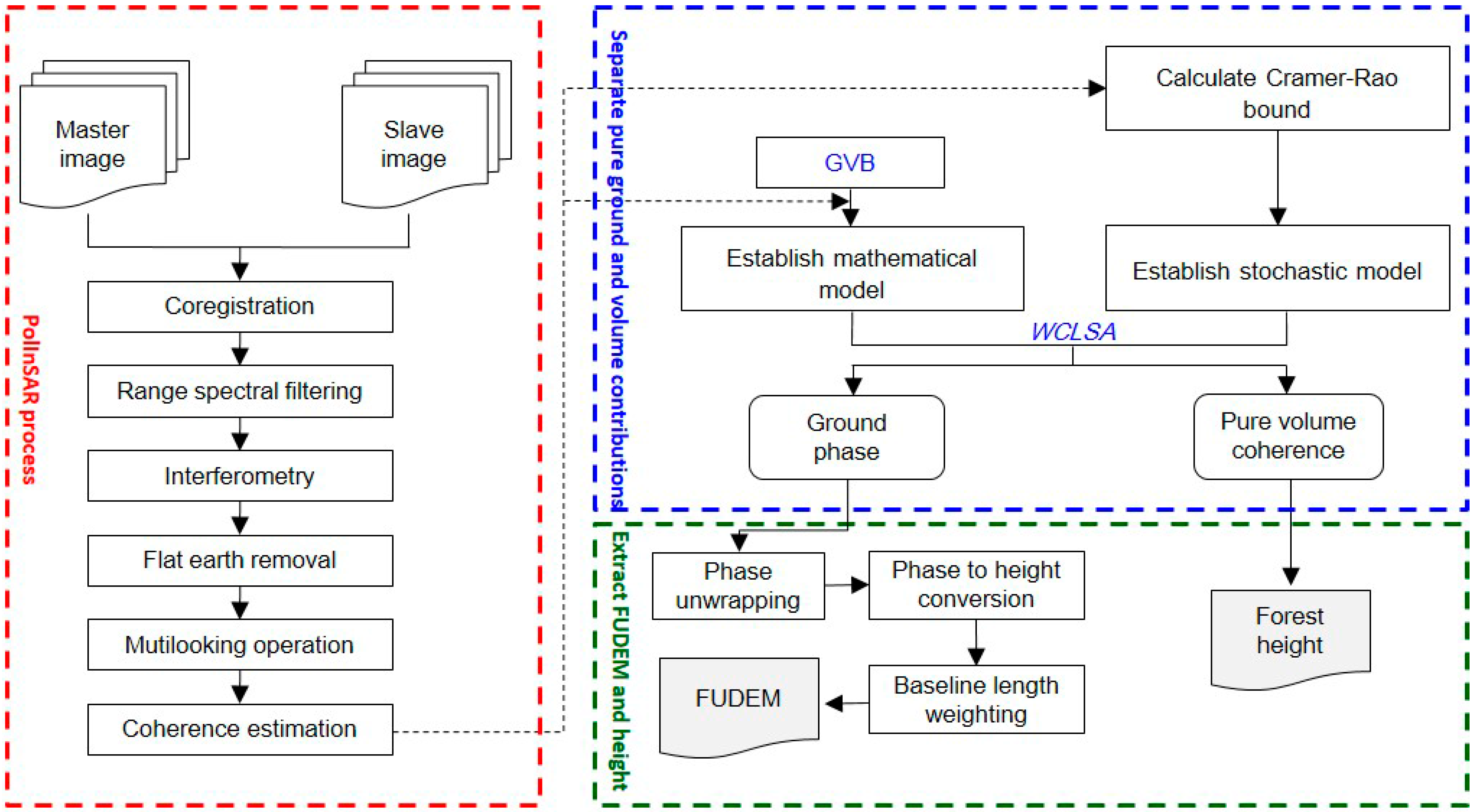
3.1. Estimations of Pure Ground and Volume Scattering Contributions with WCLSA

3.1.1. Mathematical Formulation

When considering a data-set constituted by m baselines PolInSAR data. We synthesize n interferometric coherence values by varying the polarization $\omega$ [1,5]. Thus, each coherence can be expressed as

$$\gamma ({\omega }_j^k)=f({\phi }_0^k,h_v,\delta ,\chi ,{\mu }_j^k,k_z^k)$$

(6)

where k = 1, 2, 3, $\cdots$, m and j = 1, 2, 3, $\cdots$, n. f represents the scattering model as given in Equation (4). Since the level of the temporal decorrelation is usually unknown, it is not possible to express all the ground phase with a ground height and vertical wavenumber $k_z^k$ [16,18]. Therefore, the ground phase ${\phi }_0^k$ is estimated separately for every baseline in this paper. The GVR ${\mu }_j^k$ is assumed to be constant between interferometric pairs in the same polarization. This is suitable for all interferometric pairs performed at common band, with similar incidence angles and under similar weather condition [18]. Moreover, considering the high complexity of Equation (3), ${\gamma }_v$ is parameterized by $a+bi$. Starting that every baseline has a distinct pure volume coherence ${\gamma }_v\left(a^k,b^k\right)$ caused by distinct $k_z^k$. Then, Equation (6) can be rewritten as

$$\gamma ({\omega }_j^k)=f({\phi }_0^k,{\gamma }_v^k,{\mu }_j,k_z^k)$$

(7)

Thus, before extracting the forest height and FUDEM, first we can separate the pure ground and volume contributions by estimating ${\phi }_0^k$ and ${\gamma }_v^k$. Note that, in this scheme, there are three forest parameters $\left(h_v,\delta ,\chi \right)$, which can only be inverted if at least two different PVCs are provided. In other words, we must provide at least two different interferometric pairs to invert the forest parameters.

As to the choice of n polarizations, in order to ensure that NRO ≥ 0, at least two polarizations (n ≥ 2) must be provided to obviate the rank defect of Equation (7). Furthermore, we suggest that the selected n polarizations should have distinct GVRs. The reason is that polarizations with distinct GVRs are helpful to form a well-conditioned inversion of Equation (7). For this purpose, optimum states [1] can be selected to produce a sample set in a coherence region since they tend to find the boundary revealing the shape of a coherence region [28]. As a result, compared to Pauli and linear polarizations [1], a longer visible coherence line can be observed by optimum states, which enables the estimation to be robust against the effect of coherence noise. Moreover, although increasing the number of polarizations cannot provide more redundant observations to estimate the forest parameters $\left(h_v,\delta ,\chi \right)$, it can reduce the effect of gross error in some observation on the estimations and allow us to enhance the reliability of ground phase and PVC.

3.1.2. Stochastic Model

Because the ground is strongly polarization-dependent, different polarimetric interferograms may be perturbed by different levels of noise [1,2]. Moreover, different interferometric pairs are also perturbed by different levels of noise caused by the wind-induced temporal decorrelation [29,30,31].

In order to model the contributions of observation errors to the estimations, empirical errors of the observations [4] and the COMENT method [16] have been used to estimate the covariance matrix of the observations. In this paper, the Cramer–Rao bound [1,21] is used to calculate variances of the observations and a diagonal covariance matrix can be formulated with assuming the observation errors are uncorrelated. The Cramer–Rao bound on variance of coherence magnitude can be approximately related to the coherence as [1,21]

$${\sigma }_{\left|\gamma (w)\right|}\approx \frac{1-{\left|\gamma (w)\right|}^2}{\sqrt{2N}}$$

(8)

where N is the number of independent samples used to estimate the coherence. Next, we adjust the contributions of the different interferometric coherences through ${\sigma }_{\left|\gamma (w)\right|}$. The higher the interferometric coherence, the smaller the variance, and the larger the weight. The corresponding expression is

$$p(w)=\frac{\min ({\sigma }_{\gamma (w)}^2)}{{\sigma }_{\gamma (w)}^2}$$

(9)

where $p(w)$ is the weight associated with the interferometric coherence of $\omega$.

3.1.3. Parameter Estimation

The complex least squares [32] can preserve many of the original attributes of the interferometric coherences, while reducing the disturbance of the observation errors. This approach has been widely used in model-based PolInSAR and SAR tomography inversion procedures [2,4,33,34,35]. Based on the complex least squares, the inversion algorithm for Equation (7) can be formulated as

$${\displaystyle \sum _{j=1}^m{\displaystyle \sum _{k=1}^n{\left(\gamma ({\omega }_j^k)-\widehat{\gamma }({\omega }_j^k)\right)}^H{p}_j^k\left(\gamma ({\omega }_j^k)-\widehat{\gamma }({\omega }_j^k)\right)}}=Q$$

(10)

where $\widehat{\gamma }({\omega }_j^k)$ is the observation measured by PolInSAR. ^H represents the complex conjugate transpose. $p_j^k$ represents the weight of observation $\widehat{\gamma }({\omega }_j^k)$ and can be estimated by Equation (9). For estimation scenario like Equation (10), non-linear least squares has been widely adopted to enumerate the unknown parameters [2,17,18]. In fact, such problem can also be regarded as a surveying adjustment problem, which has been widely discussed in geodesy and various theories and methods have been developed to study the relationship between observation errors and unknown parameters [36]. However, the existing adjustment methods are mainly designed for real number. Therefore, in this paper, we will introduce how to solve Equation (10) with an adjustment method.

For non-linear inversion of Equation (10), one widely used approach is the linearized strategy based on the Taylor series which is adopted to expand the nonlinear function as an approximate linear function [36]. Although this expansion is valid for complex function, we should keep in mind that ${\gamma }_v$ in Equation (7) is a complex and we should make a discussion about the stringent mathematical condition imposed on the complex differentiation [32]. In order to overcome this limitation, an alternative way to avoid complex derivative is the complex ${\gamma }_v$ can be regarded as being composed of two real parameters a and b. In such way, f can be reconstructed with two real functions to express the real and imagery parts. Lastly, Equation (7) can be rewritten as

$$\{\begin{array}{c}{v_{\mathrm{Re}}}_j^k=\frac{\partial \mathrm{Re}(f)}{\partial {\phi }^k}d{\phi }^k+\frac{\partial \mathrm{Re}(f)}{\partial a^k}d{a}^k+\frac{\partial \mathrm{Re}(f)}{\partial b^k}d{b}^k+\frac{\partial \mathrm{Re}(f)}{\partial u({\omega }_j)}du({\omega }_j)+{l_{\mathrm{Re}}}_j^k\\ {v_{\mathrm{Im}}}_j^k=\frac{\partial \mathrm{Im}(f)}{\partial {\phi }^k}d{\phi }^k+\frac{\partial \mathrm{Im}(f)}{\partial a^k}d{a}^k+\frac{\partial \mathrm{Im}(f)}{\partial b^k}d{b}^k+\frac{\partial \mathrm{Im}(f)}{\partial u({\omega }_j)}du({\omega }_j)+{l_{\mathrm{Im}}}_j^k\end{array}$$

(11)

where $\partial$ represents the derivative operation and $d{\phi }^k$, $d{a}^k$, $d{b}^k$, and $du({\omega }_j)$ are the corrections of the approximations of unknown parameters. ${l_{\mathrm{Re}}}_j^k$ and ${l_{\mathrm{Im}}}_j^k$ are the differences of the real and imaginary parts between observations and model predicted values. Matrix notation is used to express Equation (11) as follows

$$\left[\begin{array}{c}{V}_{\mathrm{Re}}\\ V_{\mathrm{Im}}\end{array}\right]=\left[\begin{array}{c}{B}_{\mathrm{Re}}\\ B_{\mathrm{Im}}\end{array}\right]X-\left[\begin{array}{c}{L}_{\mathrm{Re}}\\ L_{\mathrm{Im}}\end{array}\right] s.t. {\left[\begin{array}{c}{V}_{\mathrm{Re}}\\ V_{\mathrm{Im}}\end{array}\right]}^T\left[\begin{array}{cc}P& \\ & P\end{array}\right]\left[\begin{array}{c}{V}_{\mathrm{Re}}\\ V_{\mathrm{Im}}\end{array}\right]=\min$$

(12)

Actually, from Equation (12), we can conclude that Equation (10) is equal to a combined adjustment of complex real and imaginary parts. In addition, the weight $p_j^k$ in Equation (10) accounts for the noise contribution of a complex coherence, which is equal to set the common weight for the real and imaginary parts in Equation (12). In such way, the complex least squares in Equation (10) is converted to a least squares of real case and we can extend the surveying adjustment method into such inversion. The WCLS solution can be obtained directly from Equation (12) [36]

$$X={\left(B^{T}WB\right)}^{-1}{B}^{T}WL with W=\left[\begin{array}{cc}P& \\ & P\end{array}\right]$$

(13)

However, we find matrix B in Equation (13) is sparse and ill-conditioned, which results in an unstable estimation of $X$. The Butterworth singular value decomposition (B-SVD) [37] is applied to estimate $X$ in order to overcome the above-mentioned limitation. By B-SVD, the $X$ can be estimated with

$$X=B_1^{+}{L}_1 with \{\begin{array}{c}{B}_1=D^{-1}B\\ L_1=D^{-1}L\end{array}$$

(14)

where $B_1^{+}$ is the Moore–Penrose inverse of $B_1$ and D is the Cholesky decomposition of W⁻¹. We recommend using iterative WCLS to calculate the unknown parameters because the start values are just initial guesses. To provide the start value as accurate as possible, a simple but well-defined approach described by Equations (8.47–8.50) in [1] is recommend to calculate the initial values. If we have other reliable constraint conditions about the domain of the unknown parameters, these can also be easily embedded into Equation (12a) to enhance the inversion procedure [36,38]. Thus, we complete the GVB model inversion procedure with the WCLSA method.

3.2. Extraction of Forest Height and Underlying DEM

The ground phases and PVCs can be estimated using Equation (13). In this section, we will introduce the extraction of FUDEM and forest height with the estimated ground phases and PVCs.

3.2.1. Forest Underlying DEM Reconstruction

m ground phases can be generated with Equation (13) from the m baselines PolInSAR data. After ground interferometric phase filtering [39], phase unwrapping [40], removing the residual flat-earth phase [41,42] and phase to height conversion [43,44,45,46], m ground phases can be used to generate m FUDEMs. In order to reduce the residual random errors in the original FUDEMs, a baseline length weighting [7,47] is utilized to fuse these FUDEMs.

3.2.2. Forest Height Inversion

Using the estimated pure volume coherence, the forest height inversion can be transformed to the following nonlinear complex least squares problem

$${\displaystyle \sum _{k=1}^m{\left|{\gamma }_v^k-{\widehat{\gamma }}_v^k\right|}^2=\min }$$

(15)

where ${\widehat{\gamma }}_v^k$ denotes the estimation of ${\gamma }_v^k$ which is described in Equation (3). Considering the high complexity of Equation (3), the Nelder–Mead simplex method [48], a derivative-free method, is used for this optimization problem. In order to avoid obtaining non-physical or local solutions from Equation (15), the corresponding starting values and constraints should be carefully considered. In this paper, for the starting values, the three-stage method is adopted to roughly calculate the forest height h_v0 with SB PoInSAR data. The other two starting values of Gaussian parameters (${\delta }_0$ and ${\chi }_0$) can be respectively calculated with two empirical models designed for pine forest as presented in [11]. Then, the constraint of forest height is set by $0.5h_{v0}\le h_{v0}\le 1.5h_0$ since the forest height derived by the three-stage method is usually higher than the half of the forest and lower than the top of the forest. Finally, the constraints of the two Gaussian parameters can also be set according to the empirical models in [11] and the constraint of forest height. As a result, for each pixel of the PolInSAR image, starting values and constraints can be set adaptively.

Finally, we summarize the overall process of the WCLSA method into a three-step flowchart shown in Figure 3. The first step is the PolInSAR process [1] as shown in the red box, including coregistration, range spectral filtering, interferometry, flat earth removal and coherence estimation. Then, we construct the parameter retrieval framework to estimate the pure ground and volume contributions as presented in the blue box. Finally, the extraction of FUDEM and height is estimated through the process listed in the green box.

3.3. Simulated Experiment

3.3.1. Simulated Data

To evaluate the performance of the WCLSA method in estimating the ground and volume scattering contributions, a simulated experiment is conducted in the following scenario. Seven forest heights ranging from 5 to 35 m in combination with an elevation of the strongest backscatter power $\delta =h_v/4$ and a standard deviation $\chi =h_v/12$ are set for simulating the forest scenario. A GVR spectrum with 0.2, 0.4, 0.6, 0.8 and 1 is used to depict the polarization diversity. A k_z spectrum with 0.05, 0.075 and 0.10 is applied to simulate a three-baseline PolInSAR configuration. Using the scattering model in Equation (4), we calculate the expected interferometric coherences for the seven different forest heights. Then the three groups of interferometric coherences are, respectively, perturbed with a magnitude standard derivation (std) of 5%, 10% and 15%, and a phase std is calculated with the Cramer–Rao bound using 121 independent statistics looks [2]. Thus, an inversion framework characterized by 14 unknowns and 16 residual observations is completed.

Five hundred times of simulation experiments have been carried out with a random number generator. For comparison, we also adopt the three-stage method to independently estimate the ground phase and PVC for every baseline [13]. The coherence characterized by GVR of 0.2 is regarded as the volume dominated coherence and utilized to estimate the PVC by the three-stage method. Then, the FUDEM and forest height have been estimated following the process demonstrated in the green box of Figure 3.

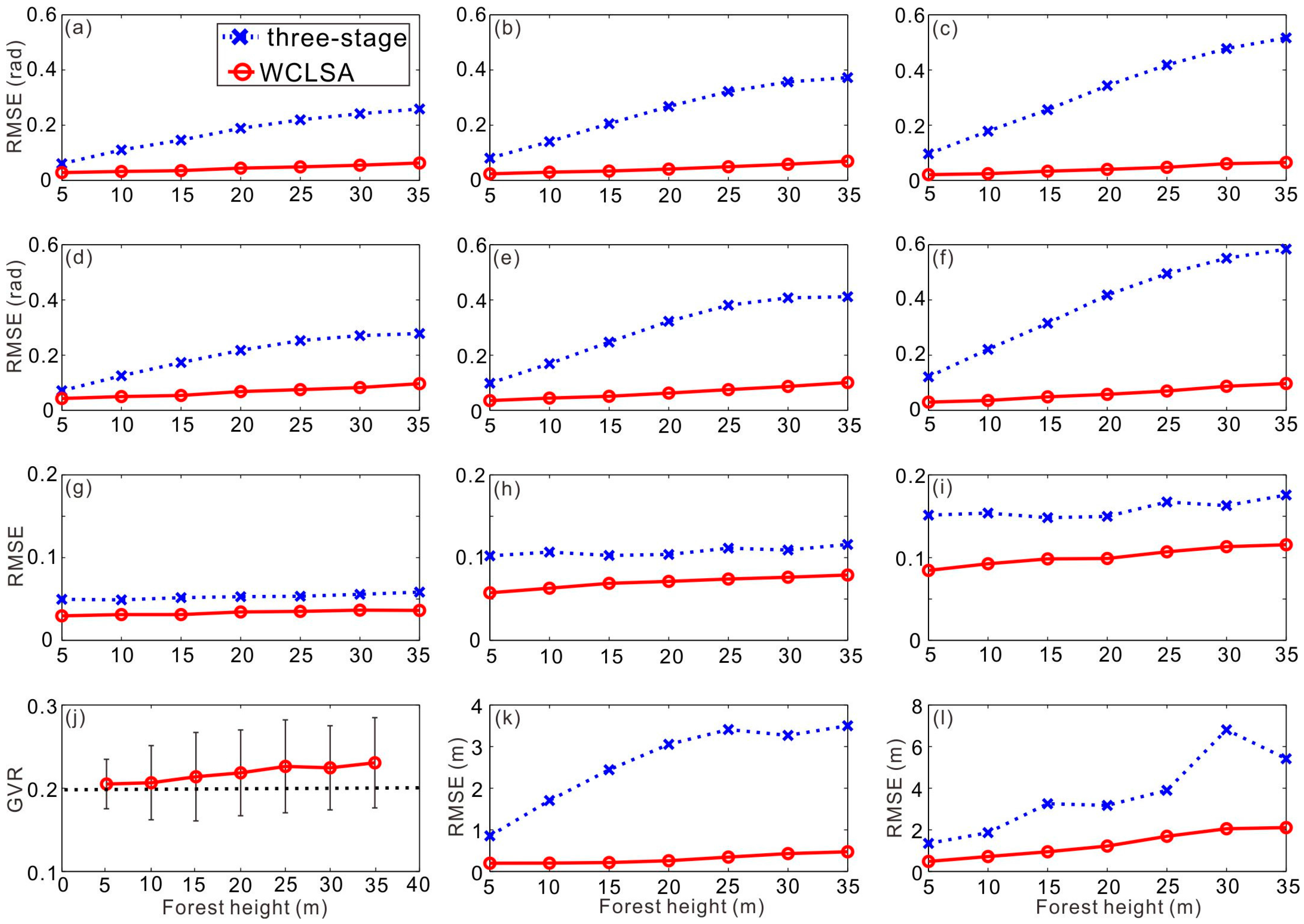
3.3.2. Results and Analysis

Figure 4 shows the root mean square errors (RMSEs) of the ground phases (Figure 4a–c), the PVC phases (Figure 4d–f) and the PVC amplitudes (Figure 4g–i). It can be observed that the WCLSA solutions have significant improvements on RMSEs in the ground phase and PVC aspects. This demonstrates that the WCLSA is superior to the three-stage method in estimating the pure ground and volume contributions. Furthermore, it can be noted that in Figure 4a–i the RMSEs of the three-stage solutions increase with the stds of the coherence magnitudes. However, the amplifications are smaller for the WCLSA solutions, which indicates that the proposed stochastic model is very helpful to scale the contributions of different coherences contaminated by different level noises. Moreover, when using the three-stage method to estimate PVC, the GVR should be assumed to be 0, which is unnecessary for the WCLSA. The GVR estimates and their RMSEs (error bars) of this simulated experiment are displayed in Figure 4j. The estimates range from 0.20 to 0.23, which is a prerequisite to secure the accuracy of the PVC estimation. Finally, following the process presented in the green box of Figure 3, the FUDEMs and forest heights are estimated. The RMSEs of FUDEMs and forest heights are displayed in Figure 4k,l, respectively. Obviously, a considerable improvement has been acquired by the WCLSA, attributing to its distinguishing capacity of estimating the ground and volume scattering contributions. Quantitatively, the RMSE of FUDEM and forest height are improved by 87% and 64%, respectively.

4. Validation with E-SAR P-Band SAR Data

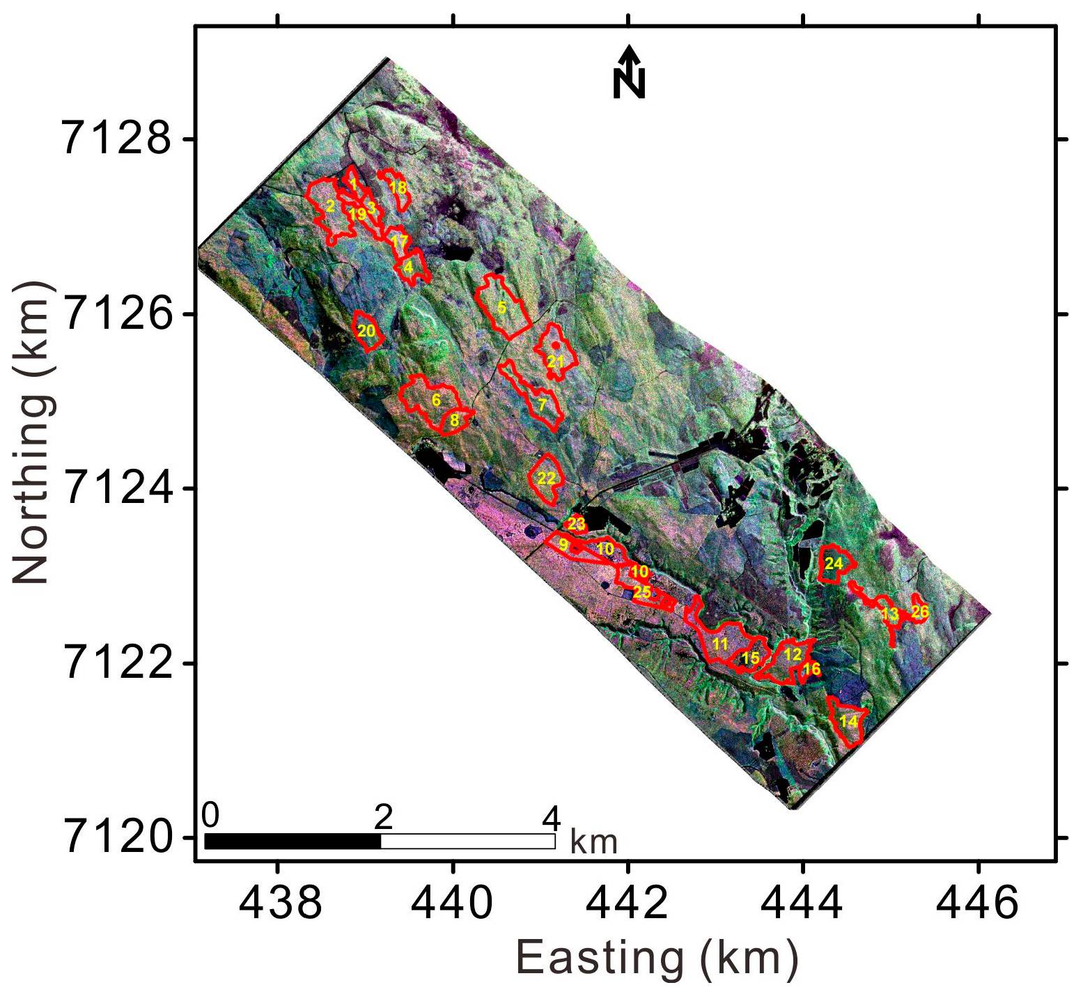
4.1. Study Area and Experimental Data

The proposed WCLSA method is also applied to the airborne P-band SAR data acquired by the German Aerospace Center (DLR)’s E-SAR sensor. The data acquisition took place in the frame of the BioSAR2008 campaign. The test site, the Krycklan Catchment, located in Northern Sweden, is mainly covered by mixed boreal forests. The topography elevation ranges from about 150 to 380 m above the sea level. In the look direction (South West), the terrain slope ranges from −10 to 10 degrees. Positive slopes are tilted towards the radar and negative slopes are titled away from the radar. The fully polarimetric SAR data set was acquired in the repeat-pass configuration. The corresponding Pauli RGB composition image is shown in Figure 5. The ground truth data of 26 forest stands (outlined in red in Figure 5) are available, including tree species, stems, average age, and biomass. In this paper, four tracks as shown in

Table 1. Parameters of airborne interferometric pairs.

Track	Temporal Baseline (min)	Baseline (m)	kz Range
1	master		master
2	32	16	0.012–0.073
3	53	24	0.024–0.135
4	70	32	0.051–0.181

are selected for constituting three baselines: 1–2, 1–3, and 1–4. In addition, as a part of the BioSAR2008 campaign, light detection and ranging (LiDAR) measurements were performed by the Swedish Defense Research Agency (FOI). The derived FUDEM and forest height will be regarded as the reference in the following sections.

4.2. Results

Following the steps presented in the red box of Figure 3, the PolInSAR process is carried out respectively to the three baselines as introduced in Table 1. As multiplicative factors of the ground and volume scattering contributions, temporal decorrelation cannot be eliminated by WCLSA since the complex least squares adjustment can only reduce the random error. In order to reduce the effect of temporal decorrelation on the interferometric coherence and to provide observations as accurate as possible, Phase diversity (PD) [49] and magnitude diversity [2] optimization methods are adopted to estimate the canopy-dominated and ground-dominated coherences. However, if the temporal decorrelation can be well modeled or compensated with a priori knowledge, the Pauli and linear polarizations can also be selected. Thus, for every baseline, five polarimetric vectors can be used to calculate the complex interferometric coherences. Then, the inversion framework can be organized by constructing 30 equations, composed of 14 unknown parameters and NRO of 16 for each resolution cell.

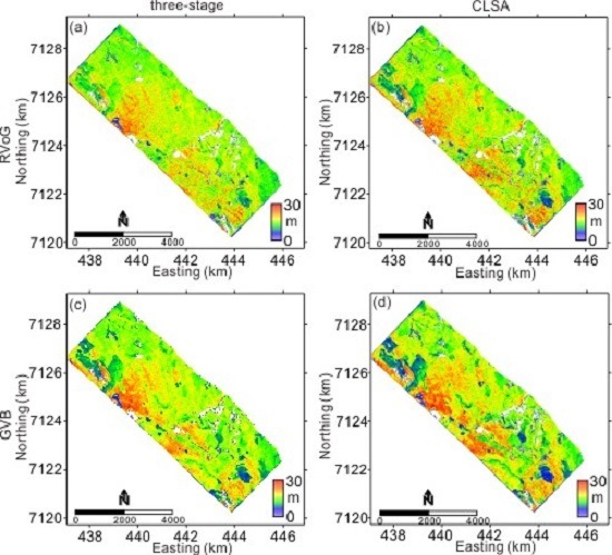
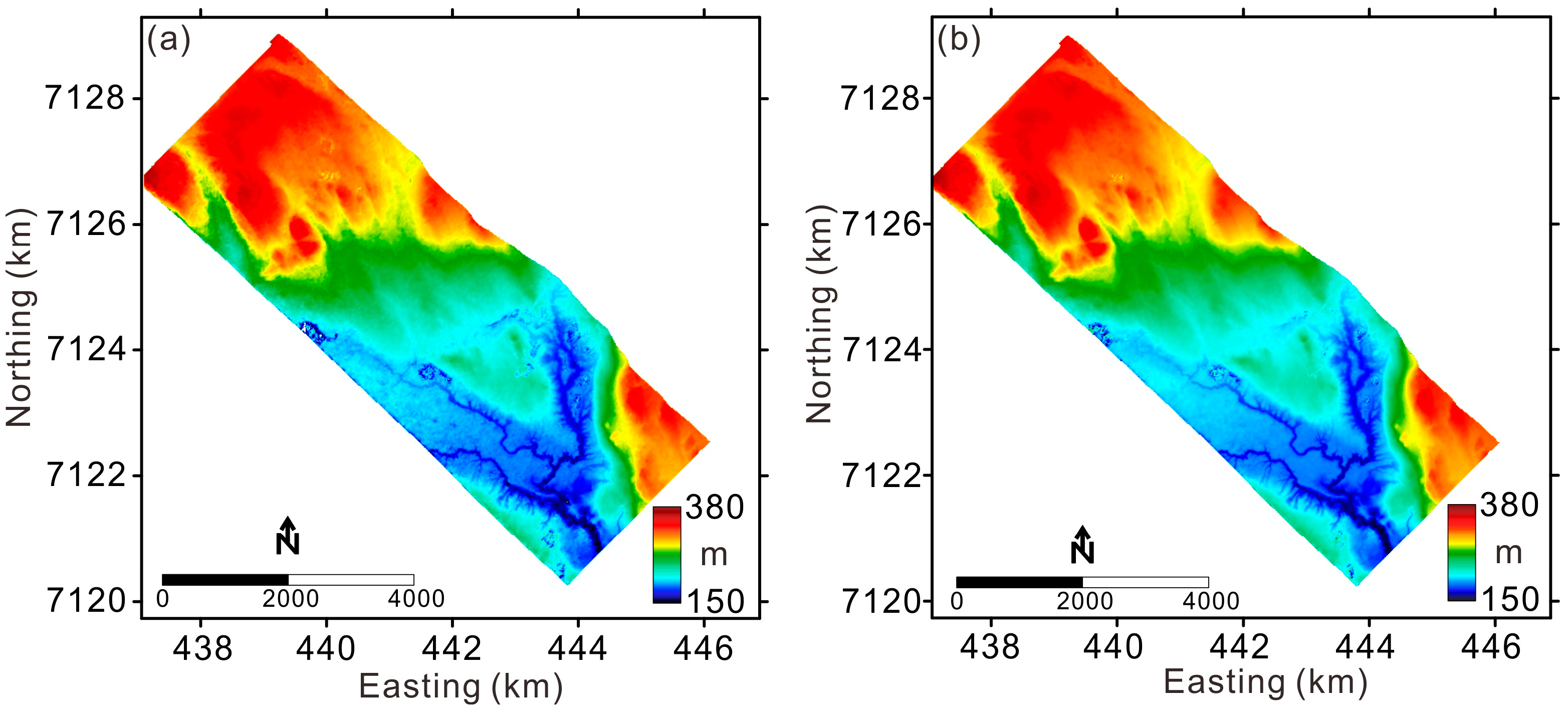
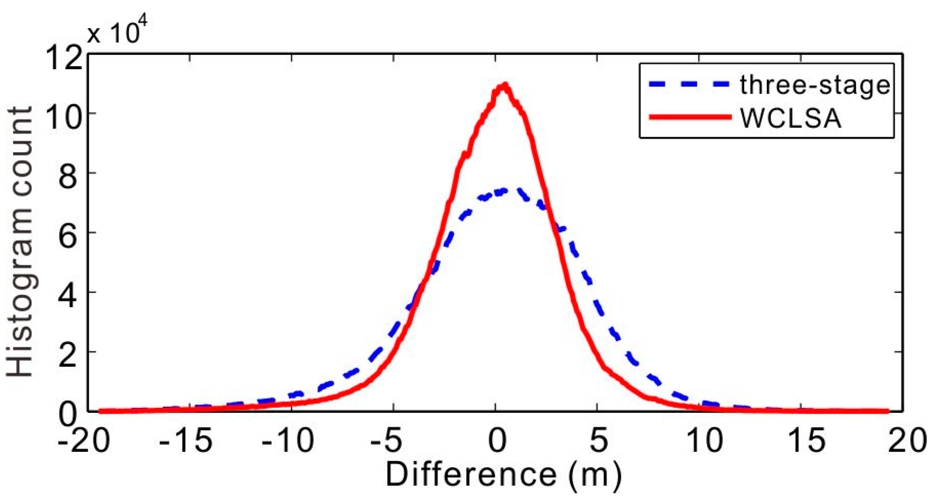
4.2.1. FUDEM Estimations

In this paper, the ground-dominated coherences estimated by the magnitude diversity approach [2] are used in phase filtering and phase unwrapping for each baseline. After phase unwrapping and residual flat-earth removal [41,42], the processed ground phases derived by the three-stage and WCLSA method are individually applied to estimate the FUDEMs. For this dataset, a two-order Rational Polynomial Coefficient model [46] is selected for a phase to height conversion. One hundred ground control points uniformly covering the range of image are extracted from the LiDAR FUDEM for calculating the RPC model. Therefore, every ground control point grid is composed of 300 × 300 pixels. Lastly, the FUDEMs are extracted as shown in Figure 6. In order to validate them, the LiDAR FUDEM is selected as the reference. The histograms of the differences between the two FUDEMs and LiDAR FUDEM are displayed in Figure 7. Compared with the LiDAR FUDEM, the two estimated FUDEMs show visible errors varying in the range of ±20 m. It can be observed that the difference relative to the three-stage FUDEM is larger than those of the WCLSA FUDEM. The RMSE for the three-stage FUDEM is 4.48 m. For the WCLSA FUDEM, it is 3.45 m, which improves the respective results by 23.0% compared with the three-stage inversion.

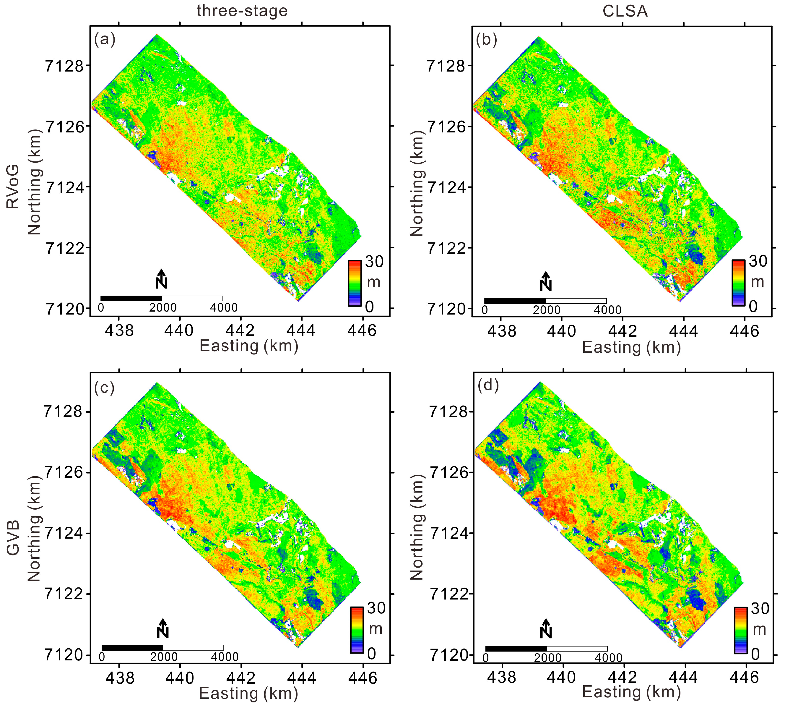
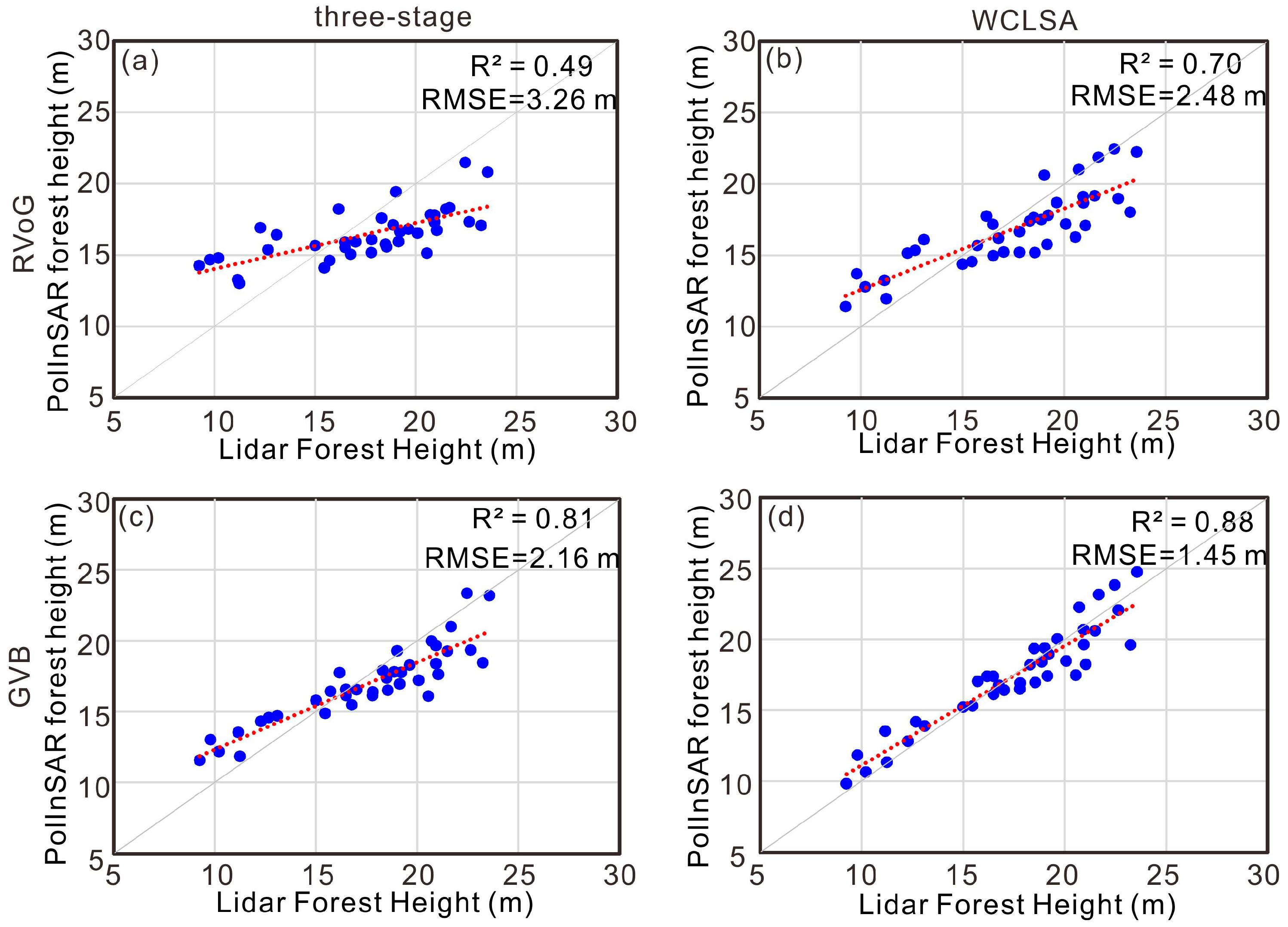
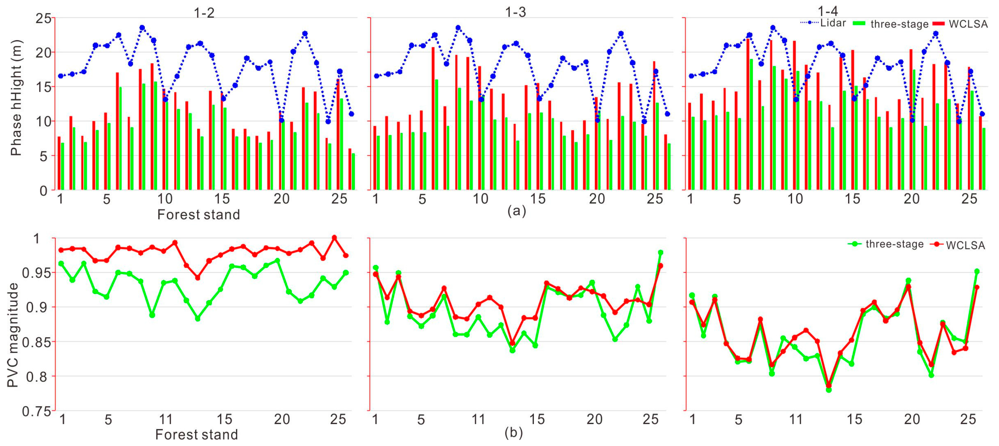
4.2.2. Forest Height Estimations

According to Equation (15), we estimate the forest height derived by the three-stage and WCLSA method with the RVoG model (Figure 8a,b) and the GVB model (Figure 8c,d). All results follow a similar spatial trend, but significant differences appear in the lowest forests. Thirty-eight forest stands (including the 26 above), characterized by nearly uniform tree heights, are selected from the LiDAR forest height. We only take the estimated forest height average for every stand. The corresponding validated stand-level plots are displayed in Figure 9. The RMSE and correlation coefficient R² are adopted to validate their performance in deriving forest height. In the RVoG-based case, the validated plots of the three-stage and WCLSA method are characterized by correlation coefficient R² values of 0.49 and 0.70, whose RMSEs are 3.26 and 2.47 m, respectively. For the GVB-based inversion, the correlation coefficient R² values are 0.81 and 0.88, whose RMSEs are 2.16 and 1.45 m, respectively. Obviously, the accuracy of GVB-based inversion is higher than that of the RVoG-based inversion. Therefore it is possible to state the following: the GVB-based forest inversion is more suitable to model the forest vertical structure in this test site. In the WCLSA inversion algorithm, the differences of PolInSAR forest heights and LiDAR forest heights have been reduced by 21.8% and 29.2%, respectively, for RVoG and GVB with an average improvement of 26.0% compared to the three-stage inversion framework. This result confirms that the WCLSA is superior to the three-stage method in case of forest height inversion.

5. Discussions

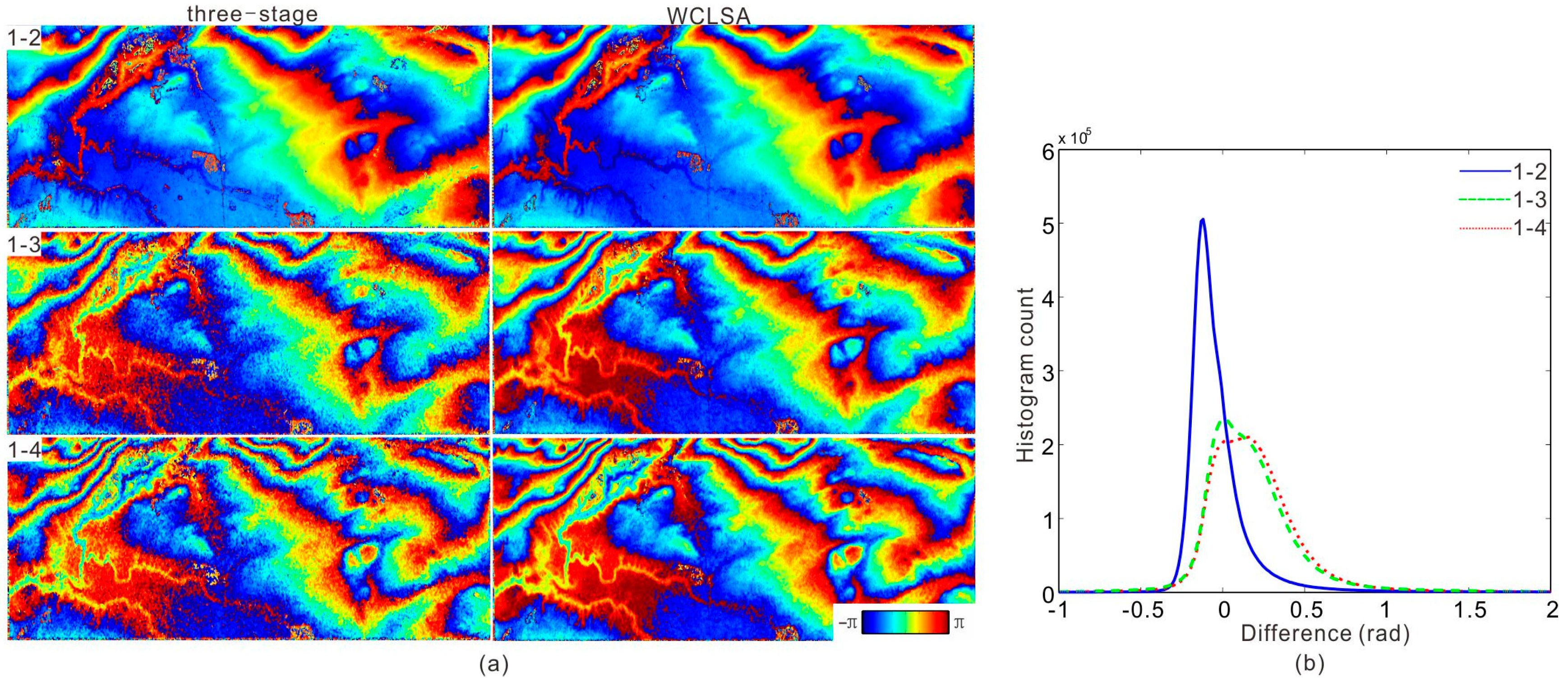
5.1. Difference of Ground Interferometric Phase

Figure 10a shows the maps of ground phases derived by the three-stage (left) and the WCLSA (right) respectively. Both of the two kinds of ground phases present similar phase patterns caused by topography. Visual comparison of ground phase maps shows that the WCLSA ground phases have clearer fringes. In order to visualize the difference, the histograms of the ground phases’ differences are shown in Figure 10b. Quantitatively, the global mean values for the three baselines are −0.02 rad (with one std = 0.30 rad), 0.30 rad (with one std = 0.34 rad) and 0.18 rad (with one std = 0.36 rad). It can be found that the difference increases with baseline and temporal baseline. The reason is that larger baselines and temporal baselines lead to more significant volume decorrelation and temporal decorrelation, respectively. Consequently, this induces lower coherence and noisier phase. As demonstrated in the simulated experiment, the nosier the observation is, the noisier the estimation is, and the WCLSA makes it possible to overcome this limitation.

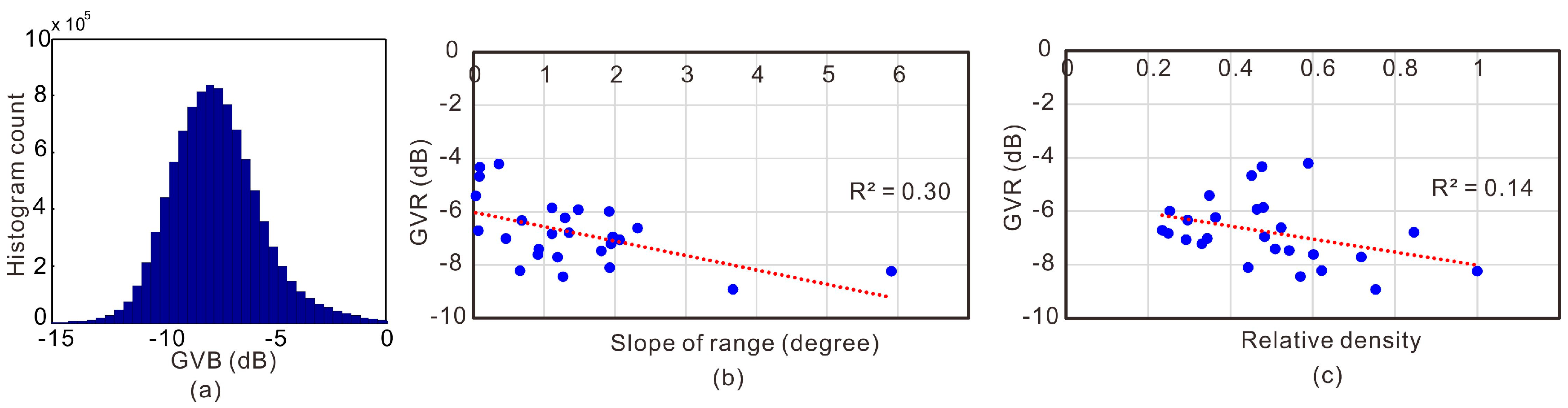
5.2. Interpretation of GVR Based on Terrain Slope and Forest Density

The GVR of PD_High polarization (volume dominated polarization) [49] reported in the histogram of Figure 11a ranges from −15 to 0 dB and is characterized by a global mean of −7.6 dB. For the selected 26 forest stands outlined in Figure 5, the maximal mean of GVRs is up to −4.5 dB, almost three times higher than the minimal mean of GVRs (−9 dB). Even though the coherence optimization methods have been adopted to estimate the ground and the volume scattering contribution, it is still hard to ensure that the GVR is less than −10 dB. On the other hand, it also implies that P band data present good visibility of the ground over boreal forests.

As discussed in RVoG assumption [1,2], the ground scattering contribution is mainly induced by the odd-bounce scattering and the double-bounce scattering. Both of the scattering mechanisms are significantly affected by the range terrain slope [50]. In particular, odd-bounce scattering intensity increases with positive range slope and decreases with negative range slope, while double-bounce scattering intensity decreases with range slope since the range slope distorts the geometry of the double-bounce scattering at the base of trees. However, in this experiment, we have not observed that GVR significantly increases with the positive range slope. Conversely, Figure 11b shows that the GVR decreases with the absolute range slope and the correlation coefficient R² is about 0.30. In particular, the correlation coefficient R² (0.27) is smaller than 0.30 when the range slope is smaller than 2.5 degree, which means that the ground scattering contribution is affected less by the range slope smaller than 2.5 degree for this test site. However, when the range slope is larger than 2.5 degree, the ground scattering contribution decreases significantly. It may suggest that the ground scattering contribution is mainly attributed to double-bounce scattering and the phase centers of odd-bounce scattering may not locate at the underlying ground. The method proposed in [51] may help identifying the phase centers of the forest scattering mechanisms and gasp an advanced understanding of the relationship between the GVR and the slope. In addition, azimuth slope also has influence on the forest scattering mechanisms [50], but no definitive conclusions about the relationships between GVR and azimuth slope could be drawn in this paper.

It can be seen in Figure 11c that the GVR decreases with the increasing forest density. Compared with dense forest, more important ground scattering (e.g., double-bounce scattering) occurs in the sparse forest since the electromagnetic wave undergoes a decrease of attenuation when it propagates into the forest layer. However, we note that the correlation coefficient R² between GVR and forest density is just 0.14, which illustrates that the GVR is not highly correlated with the forest density for this test site. It can be explained by the fact that the forest density used in this paper may not well reflect the number of trucks, which has a strong correlation with the attenuation of an electromagnetic wave [27,52]. This may be suitable for managed forests with similar ages where the number of trucks increases with the forest density. Moreover, for P band PolInSAR data, while the main scattering elements are large-scale trucks whose lengths change with the ages, the forest age is another important factor should be considered. Hence, more prior knowledge about forest structure is required which may help to convert forest density to trunk density is needed in order to find a better fitting relationship.

The two above findings are tentative and needed further research. However, these findings may important to grasp a better understanding of forest scattering mechanisms and refine the model-based inversion.

5.3. Effect of GVR Compensation on PVC

As mentioned in Section 2, the WCLSA method can estimate the PVC without a null GVR assumption. To visualize the effect of the GVR compensation, the PVC estimates of the 26 stands are selected for analysis. Figure 12 shows the average PVC phase height (Figure 12a) and PVC magnitude (Figure 12b) estimation of the 26 forest stands produced by the three-stage and WCLSA method. As a reference, the stand-level forest heights derived from LiDAR surveys are also provided (the blue dashed line) to evaluate the phase of PVC. The WCLSA PVC magnitudes occasionally increase or decrease compared with those of the three-stage method. However, it is impossible to access the PVC magnitudes since true reference values are unavailable in practice. In the phase aspect, for most stands in the three baselines, the WCLSA phase heights are higher and closer to the LiDAR forest heights, which denote that the WCLSA phase heights are closer to the LiDAR forest height except for the stands 10, 15 and 20. The reason may be that the GVR have been assumed to be constant within each interferometric pair, which may be insufficient for modeling the variation of the GVR. Thus, the non-modeled GVR error could influence the accuracy of the PVC.

5.4. Limitations of WCLSA

Three problems are still worth a discussing. Firstly, the constant GVR assumption may be insufficient for modeling the changes of the scattering mechanisms. The application of the WCLSA method proposed in this paper is recommended to fuse MB PolInSAR data collected with short temporal intervals. A more precise temporal GVR model is needed in the case of longer repeat-pass intervals. Secondly, the WCLSA method does not take into account the temporal decorrelation when forest parameters are estimated from repeat-pass PolInSAR data. Therefore, it is necessary to develop a temporal decorrelation model to remove the temporal decorrelation in the interferometric coherence. Finally, only the magnitude of the interferometric coherence has been adopted to commonly scale the corresponding reliability of the real and imaginary parts, which seems to be low sensitive to the distinction of the reliability of the real and imaginary parts associated with the interferometric coherence. More adaptive weighting strategy [36,38] is needed to scale the contributions of different polarizations.

6. Conclusions

We have proposed the WCLSA method based on the GVB model to invert the forest height and FUDEM using P band MB PolInSAR data. Different from the RVoG model, a Gaussian function has been adopted to depict the vertical distribution of the canopy elements in the GVB model, which is used for forest height inversion firstly. Moreover, the WCLSA method fusing the MB PolInSAR data and considering the contributions of the decorrelations to the solutions is derived for the GVB inversion. For our experiment with simulated data, we have shown that different from the three-stage method, the WCLSA method can reduce the dependence of the solutions on the decorrelations and improve the accuracy of the solutions significantly. This is also well validated with the airborne E-SAR P-band SAR data over mixed boreal forest. A FUDEM with a RMSE of 3.45 m is obtained. We have also found that the GVB is more suitable to model the scattering process of pine forest with an improvement of forest height accuracy on RMSE by 37.5%. In addition to the FUDEM and forest height, the ground phase, the ground to volume ratio and the pure volume coherence are also estimated and discussed. In order to better understand the scattering process, we should pay more attentions to the terrain slope and forest density. This will be studied in the future works.

References

1. Cloude, S.R. Polarisation: Applications in Remote Sensing; Oxford University Press: New York, NY, USA, 2009. [Google Scholar]
2. Papathanassiou, K.P.; Cloude, S.R. Single-baseline polarimetric SAR interferometry. IEEE Trans. Geosci. Remote Sens. 2001, 39, 2352–2363. [Google Scholar] [CrossRef]
3. Treuhaft, R.N.; Madsen, S.N.; Moghaddam, M.; van Zyl, J.J. Vegetation characteristics and underlying topography from interferometric data. Radio Sci. 1996, 31, 1449–1495. [Google Scholar] [CrossRef]
4. Treuhaft, R.N.; Siqueira, P.R. Vertical structure of vegetated land surfaces from interferometric and polarimetric data. Radio Sci. 2000, 35, 141–177. [Google Scholar] [CrossRef]
5. Cloude, S.R.; Papathanassiou, K.P. Polarimetric SAR interferometry. IEEE Trans. Geosci. Remote Sens. 1998, 36, 1551–1565. [Google Scholar] [CrossRef]
6. Lopez-Martinez, C.; Papathanassiou, K.P. Cancellation of scattering mechanisms in PolInSAR: Application to underlying topography estimation. IEEE Trans. Geosci. Remote Sens. 2013, 51, 953–965. [Google Scholar] [CrossRef]
7. Iribe, K.; Lopez-Martinez, C.; Papathanassiou, K.P.; Hajnsek, I. Estimation of ground topography in forested terrain by means of Pol-InSAR. In Proceedings of the 2008 IEEE International Geoscience and Remote Sensing Symposium, Boston, MA, USA, 6–11 July 2008.
8. Mercer, B.; Zhang, Q.; Schwaebisch, M.; Denbina, M.; Cloude, S.R. Forest height and ground topography at L-band from an experimental single-pass airborne Pol-InSAR system. In Proceeding of the PolInSAR Workshop, Frascati, Italy, 26–31 January 2009.
9. Kugler, F.; Schulze, D.; Hajnsek, I.; Pretzsch, H.; Papathanassiou, K.P. TanDEM-X Pol-InSAR performance for forest height estimation. IEEE Trans. Geosci. Remote Sens. 2014, 52, 6404–6422. [Google Scholar] [CrossRef]
10. Garestier, F.; Dubois-Fernandez, P.C.; Papathanassiou, K.P. Pine forest height inversion using single-pass X-band PolInSAR data. IEEE Trans. Geosci. Remote Sens. 2008, 46, 56–68. [Google Scholar] [CrossRef] [Green Version]
11. Garestier, F.; le Toan, T. Forest modeling for height inversion using single baseline InSAR/Pol-InSAR data. IEEE Trans. Geosci. Remote Sens. 2010, 48, 1528–1539. [Google Scholar] [CrossRef]
12. Garestier, F.; le Toan, T. Estimation of the backscatter vertical profile of a pine forest using single baseline P-band (Pol-) InSAR data. IEEE Trans. Geosci. Remote Sens. 2010, 48, 3340–3348. [Google Scholar] [CrossRef]
13. Cloude, S.R.; Papathanassiou, K.P. Three-stage inversion process for polarimetric SAR interferometry. Proc. Inst. Electr. Eng. Radar Sonar Navigat. 2003, 150, 125–134. [Google Scholar] [CrossRef]
14. Garestier, F.; Dubois-Fernandez, P.C.; Guyon, D.; le Toan, T. Forest biophysical parameter estimation using L- and P-band polarimetric SAR data. IEEE Trans. Geosci. Remote Sens. 2009, 47, 481–492. [Google Scholar] [CrossRef]
15. Garestier, F.; Dubois-Fernandez, P.C.; Champion, I. Forest height inversion using high resolution P-band Pol-InSAR data. IEEE Trans. Geosci. Remote Sens. 2008, 46, 3544–3559. [Google Scholar] [CrossRef]
16. Tebaldini, S. Multi-Baseline SAR Imaging: Models and Algorithms. Ph.D. Thesis, Politecnico Di Milano, Milano, Italy, 11 October 2009. [Google Scholar]
17. Neumann, M.; Ferro-Famil, L.; Reigber, A. Estimation of forest structure, ground and canopy layer characteristics from multi-baseline polarimetric interferometric SAR data. IEEE Trans. Geosci. Remote Sens. 2010, 48, 1086–1104. [Google Scholar] [CrossRef]
18. Lavalle, M.; Khun, K. Three-baseline InSAR estimation of forest height. IEEE Geosci. Remote Sens. Lett. 2014, 11, 1737–1741. [Google Scholar] [CrossRef]
19. Kugler, F.; Lee, S.; Papathanassiou, K.P. Estimation of forest vertical structure parameter by means of multi-baseline Pol-InSAR. In Proceeding of the PolInSAR Workshop, Frascati, Italy, 26–31 January 2009.
20. Lee, S.; Kugler, F.; Papathanassiou, K.P.; Hajnsek, I. Multibaseline polarimetric SAR interferometry forest height inversion approaches. In Proceeding of the 8th European Conference on Synthetic Aperture Radar, Aachen, Germany, 7–10 June 2010.
21. Lee, J.; Hoppel, K.; Mango, S.; Miller, A. Intensity and phase statistics of multilook polarimetric and interferometric SAR image. IEEE Trans Geosci Remote Sens. 1994, 32, 1017–1028. [Google Scholar]
22. Saleh, K.; Porte, A.; Guyon, D.; Ferrazzoli, P.; Wigneron, J.-P. A forest geometric description of a maritime pine forest suitable for discrete microwave models. IEEE Trans. Geosci. Remote Sens. 2005, 43, 2024–2035. [Google Scholar] [CrossRef]
23. Ballester-Berman, J.D.; Vicente-Guijalba, F.; Lopez-Sanchez, J.M. A simple RVoG test for PolInSAR data. IEEE J. Sel. Top. Appl. Earth Obs. Remote Sens. 2015, 8, 1028–1040. [Google Scholar] [CrossRef]
24. Le Toan, T.; Quegan, S.; Davidson, M.W.J.; Balzter, H.; Paillou, P.; Papathanassiou, K.P.; Plummer, S.; Rocca, F.; Saatchi, S.; Shugart, H.; et al. The BIOMASS mission: Mapping global forest biomass to better understand the terrestrial carbon cycle. Remote Sens. Environ. 2011, 115, 2850–2860. [Google Scholar] [CrossRef]
25. Dubois-Fernandez, P.; Souyris, J.C.; Angelliaume, S.; Garestier, F. The compact polarimetry alternative for spaceborne SAR at low frequency. IEEE Trans. Geosci. Remote Sens. 2008, 46, 3208–3222. [Google Scholar] [CrossRef]
26. Hajnsek, I.; Kugler, F.; Lee, S.K.; Papathanassiou, K.P. Tropical-forest-parameter estimation by means of Pol-InSAR: The INDREX-II campaign. IEEE Trans. Geosci. Remote Sens. 2009, 47, 481–492. [Google Scholar] [CrossRef]
27. Wang, C.; Wang, L.; Fu, H.; Xie, Q.; Zhu, J. The Impact of Forest Density on Forest Height Inversion Modeling from Polarimetric InSAR Data. Remote Sens. 2016, 8, 291. [Google Scholar] [CrossRef]
28. Flynn, T.; Tabb, M.; Carande, R. Coherence region shape extraction for vegetation parameter estimation in polarimetric SAR interferometry. In Proceedings of the 2002 IEEE International Geoscience and Remote Sensing Symposium, Westin Harbour Castle, Toronto, ON, Canada, 24–28 June 2002; pp. 2596–2598.
29. Lavalle, M.; Simard, M.; Hensely, S. A temporal decorrelation model for polarimetric radar interferometers. IEEE Trans. Geosci. Remote Sens. 2012, 50, 2880–2888. [Google Scholar] [CrossRef]
30. Ahmed, R.; Siqueira, P.; Hensley, S.; Chapman, B.; Bergen, K. A survey of temporal decorrelation from spaceborne L-band repeat-pass InSAR. Remote Sens. Environ. 2011, 115, 2887–2896. [Google Scholar] [CrossRef]
31. Papathanassiou, K.P.; Cloude, S.R. The effect of temporal decorrelation on the inversion of forest parameters from Pol-InSAR data. In Proceedings of the 2003 IEEE International Geoscience and Remote Sensing Symposium, Toulouse, France, 21–25 July 2003; pp. 1429–1431.
32. Miller, K.S. Complex linear least squares. Siam Rev. 1973, 15, 706–725. [Google Scholar] [CrossRef]
33. Fu, H.; Wang, C.; Zhu, J.; Xie, Q.; Zhao, R. Inversion of forest height from PolInSAR using complex least squares adjustment method. Sci. China Earth Sci. 2015, 58, 1018–1031. [Google Scholar] [CrossRef]
34. Tebaldini, S. Single and multipolarimetric SAR tomography of forested areas: A parametric approach. IEEE Trans. Geosci. Remote Sens. 2010, 48, 2375–2387. [Google Scholar] [CrossRef]
35. Tebaldini, S.; Rocca, F. Multibaseline polarimetric SAR tomography of a boreal forest at P- and L-bands. IEEE Trans. Geosci. Remote Sens. 2012, 50, 232–246. [Google Scholar] [CrossRef]
36. Cui, X.; Yu, Z.; Tao, B.; Liu, D.; Yu, Z.; Sun, H.; Wang, X. The basic theory of robust estimation. In Generalized Surveying Adjustment, 2nd ed.; Wuhan University Press: Wuhan, China, 2009; pp. 186–201. [Google Scholar]
37. Wei, L.; Balz, T.; Liao, M.; Zhang, L. TerraSAR-X Stripmap Data Interpretation of Complex Urban Scenarios with 3D SAR Tomography. J. Sens. 2014, 2014, 386753. [Google Scholar] [CrossRef]
38. Hu, J.; Li, Z.; Sun, Q.; Zhu, J.; Ding, X. Three-dimensional surface displacements from InSAR and GPS measurements with variance component estimation. IEEE Geosci. Remote Sens. Lett. 2014, 9, 754–758. [Google Scholar]
39. Li, Z.; Ding, X.; Huang, C.; Zhu, J.; Chen, Y. Improved filtering parameter determination for the Goldstein radar interferogram filter. ISPRS J. Photogramm. Remote Sens. 2008, 63, 621–634. [Google Scholar] [CrossRef]
40. Chen, C.; Zebker, H. Two-dimensional phase unwrapping with use of statistical models for cost function in nonlinear optimization. J. Opt. Soc. Am. A 2001, 18, 338–351. [Google Scholar] [CrossRef]
41. Feng, G.; Ding, X.; Li, Z.; Jiang, M.; Zhang, L.; Omura, M. Calibration of an InSAR-derived coseimic deformation map associated with the 2011 Mw-9.0 Tohoku-Oki Earthquake. IEEE Trans. Geosci. Remote Sens. Lett. 2012, 9, 302–306. [Google Scholar] [CrossRef]
42. Xu, B.; Li, Z.; Wang, Q.; Jiang, M.; Zhu, J.; Ding, X. A refined strategy for removing composite errors of SAR interferogram. IEEE Geosci. Remote Sens. Lett. 2014, 11, 143–147. [Google Scholar] [CrossRef]
43. Small, D. Generation of Digital Elevation Models through Spaceborne SAR Interferometry. Ph.D. Thesis, University of Zurich, Zurich, Swizerland, 1998. [Google Scholar]
44. Reigber, A.; Prats, P.; Mallorqui, J.J. Refined estimation of time-varying baseline errors in airborne SAR interferometry. IEEE Geosci. Remote Sens. Lett. 2006, 3, 145–149. [Google Scholar] [CrossRef]
45. Zhang, G.; Fei, W.; Li, Z.; Liu, Z.; Li, D. Evaluation of the RPC model as a replacement for the spaceborne InSAR phase equation. Photogramm. Rec. 2011, 26, 325–338. [Google Scholar] [CrossRef]
46. Fei, W.; Zhang, G.; Tang, X.; Li, D.; Gao, X. Research of RPC model for DEM generation by InSAR technique. Acta Geod. Cartogr. Sin. 2014, 43, 83–88. [Google Scholar]
47. Ferretti, A.; Prati, C.; Rocca, F. Multibaseline InSAR DEM reconstruction: The wavelet approach. IEEE Trans. Geosci. Remote Sens. 1999, 37, 705–715. [Google Scholar] [CrossRef]
48. Press, W.H.; Teukolsky, S.A.; Vetterling, W.T.; Flannery, B.P. Numerical Recipes in C: The Art of Scientific Computing; Cambridge University Press: Cambridge, UK, 1992. [Google Scholar]
49. Tabb, M.; Orrey, J.; Flynn, T. Phase Diversity: An optimal decomposition for vegetation parameter estimation using polarimetric SAR interferometry. In Proceeding of the 4th European Conference on Synthetic Aperture Radar, Köln, Germany, 2–4 June 2002; pp. 721–724.
50. Park, S.-E.; Moon, W.M.; Pottier, E. Assessment of scattering mechanism of polarimetric SAR signal from mountainous forest areas. IEEE Trans. Geosci. Remote Sens. 2012, 50, 4711–4719. [Google Scholar] [CrossRef]
51. Ballester-Berman, J.D.; Lopez-Sanchez, J.M. Applying the Freeman–Durden decomposition concept to polarimetric SAR interferometry. IEEE Trans. Geosci. Remote Sens. 2010, 48, 466–479. [Google Scholar] [CrossRef]
52. Freeman, A.; Durden, S. A three-component scattering model for polarimetric SAR data. IEEE Trans. Geosci. Remote Sens. 1998, 36, 963–973. [Google Scholar] [CrossRef]
Figure 1. Geometrical interpretation of polarization coherence locus for Gaussian vertical backscatter (GVB).
Remotesensing 08 00820 g001
Figure 2. (a) Representation of interferometric coherence sets in complex plane for different GVRs; and (b) bias of the forest heights under the null GVR assumption.
Remotesensing 08 00820 g002
Figure 3. Flowchart of the proposed weighted complex least squares adjustment (WCLSA) algorithm.
Remotesensing 08 00820 g003
Figure 4. Solutions derived by three-stage and WCLSA: (ac) Root mean square errors (RMSEs) of ground phases associated with the three baselines; (df) RMSEs of phases; (gi) The magnitudes of pure volume coherences (PVCs); (j) GVR estimates and the corresponding RMSEs (error bar); and (k,l) RMSEs of the forest underlying digital elevation model (FUDEM) and forest height.
Remotesensing 08 00820 g004
Figure 5. Test site Krycklan Catchment: P-band RGB composite intensity image in the Pauli-basis, including 26 forest stands marked by red polygons.
Remotesensing 08 00820 g005
Figure 6. FUDEMs derived by: three-stage (a); and WCLSA (b).
Remotesensing 08 00820 g006
Figure 7. Differences of FUDEMs derived by three-stage and WCLSA with respect to the LiDAR DEM.
Remotesensing 08 00820 g007
Figure 8. Forest heights inverted by: three-stage and WCLSA with: random volume over ground (RVoG) model (a,b); and GVB model (c,d).
Remotesensing 08 00820 g008
Figure 9. Forest heights estimated by three-stage and WCLSA with: RVoG model (a,b); and GVB model (c,d), compared with forest height measured by LiDAR.
Remotesensing 08 00820 g009
Figure 10. (a) Maps of forest ground interferometric phase estimated by three-stage (linear fitting) and WCLSA respectively for baseline 1–2, 1–3 and 1–4; and (b) Histograms of differences between three-stage ground phases and WCLSA phases.
Remotesensing 08 00820 g010
Figure 11. GVR estimates of PDHigh polarization: (a) Histogram of GVR; (b) Joint distribution of GVR and slope of range; and (c) Joint distribution of GVR and forest density. The red dashed lines in (b,c) have been obtained through a line fit between the GVR and the forest density.
Remotesensing 08 00820 g011
Figure 12. Average PVC phase height (bar graph) (a); and PVC magnitude (b) estimates of the 26 forest stands.
Remotesensing 08 00820 g012