1. Introduction
The initial atmospheric and surface conditions are critical in the numerical weather prediction (NWP) modeling. Understanding current atmospheric and surface states potentially enhance the quality of initial fields and improve the weather forecasts. Increasing the amount of remote sensing data from satellite has been proven for this purpose. There are studies (e.g., [
1,
2,
3]) that have demonstrated that forecast skill of severe weathers, such as extreme precipitation associated with monsoon and tropical cyclones (TCs) has benefited from the assimilation of various types of satellite data. The first generation advanced infrared instrument, Atmospheric Infrared Sounder (AIRS), was successfully sent into space in 2002, followed by the Infrared Atmospheric Sounding Interferometer (IASI) and the Cross-track Infrared Sounder (CrIS) in 2006 and 2011, respectively. All these advanced infrared sounders could provide vertical profiles at higher resolution than traditional infrared instruments, in particular the cloud-free field-of-views (FOVs). In order to increase the sounding capability, they are typically used jointly with microwave instrument, such as the Advanced Microwave Sounding Unit (AMSU) and/or the Advanced Technology Microwave Sounder (ATMS), to take the all-weather advantage of both cloud-penetration and clear-sky in microwave spectral regime. Under this synergistic circumstance, the spatial resolution may downgrade from finer advanced infrared instrument at 12~15-km to coarser microwave sensor at 50-km at nadir. These joint retrievals typically follow the name from the advanced infrared sounder.
There are two approaches to merge remotely sensed data into a NWP model: assimilating the observed radiances, or assimilating the retrieved parameters such temperature and moisture profiles. Major NWP centers use satellite observed radiances into their NWP models through data assimilation technique (e.g., [
4,
5]). Using radiances in the assimilation system requires a forward calculation operator, which transfers the model physical states into the radiances space through the assistance of radiative transfer model. This requires a lot of computational resources, especially for hyperspectral instruments with thousands of channels, in order to handle the difference between observation and model states adequately. On the other hand, assimilating the retrieved physical parameters is relative straightforward and computationally efficient in a data assimilation system. Those retrieved parameters are typically important thermodynamic states, and could be compared with NWP model outputs conjunctionally through the objective analysis scheme. Recent studies have shown that assimilating retrieved products have a similar forecast impact as using observed radiance on improving the skill [
2,
6,
7,
8]. However, these studies focus on the assimilation and validation of only one type of retrieved product, and use tropical cyclones as testing cases which are known as rapidly evolving severe weather phenomena in tropical and subtropical latitudes. There is little attention paid to the use of both full-spatial-resolution advanced infrared and microwave soundings that have complementary characteristics in terms of spatial coverage and vertical resolving capability.
Since the launch of NASA’s Earth Observing System (EOS) Aqua satellite in 2002, the onboard AIRS and AMSU provide a great opportunity to address the synergistic use of both instruments. These two sensors have an identical overpass in local time and measure almost the same atmospheric column. Numerous studies have reported the positive impacts due to the use of their observations. Therefore, the objective of this study is to evaluate the optimal use of both complementary soundings from AIRS and AMSU-A to enhance the numerical forecast skill of fair transition of the atmosphere condition, such as frontal or monsoon system, in a regional scale.
In the following sections, two types of soundings are summarized in
Section 2.
Section 3 reports the results from assimilating these retrieved profiles into the Advanced Research version of the Weather Research and Forecasting (WRF) model with a three-dimensional variational (3D-var) data assimilation technique. A heavy precipitation frontal system due to monsoon over Taiwan and its surrounding will be used to evaluate the forecast performance. There are short descriptions on model configurations along with a series of cycling assimilation and forecast experiments in this section. The impact of various combinations of AIRS and AMSU soundings are shown in
Section 4. In
Section 5, we propose the optimal use of both data set and the initial evaluation on it.
Section 6 will discuss the concluding remarks and possible future work.
2. AIRS and AMSU Sounding Retrieval Systems
2.1. AIRS and AMSU Instrument
The AIRS, together with AMSU on the Aqua satellite, are designed to form a new generation polar orbiting infrared and microwave atmospheric sounding system. The primary products of AIRS and AMSU are twice daily global fields of atmospheric temperature, moisture, ozone profiles, sea/land surface skin temperature, and cloud-related parameters including outgoing longwave radiation (OLR) [
9]. The Aqua platform is a sun-synchronized polar orbit satellite at an altitude of 705 km. The scan geometries of AIRS and AMSU are with 1.1° and 3.3° footprints, which are equivalent to horizontal resolutions of 13.5 and 45 km at nadir, respectively. The AIRS measures radiances in the infrared region 3.74–15.4 μm with 2378 channels at high-spectral-resolution (
= 1200, where
is the wavenumber and
is the full-width half maximum of a channel). The AMSU is comprised of two separated sensor units, AMSU-A1 and AMSU-A2, with microwave spectral ranges of 50–90 GHz and 23–32 GHz for 13 and 2 channels. Therefore, the AMSU footprint is three times wider than the AIRS footprint and covers a cluster of nine AIRS footprints under this alignment [
10]. Data from one AMSU footprint and nine AIRS footprints are used to create a single “cloud-cleared” infrared spectrum. The cloud-cleared AIRS radiances at AMSU spatial resolution are applied in the AIRS Science Team retrieval algorithm, and are typically named as AIRS Science Team standard products. The sounding goals of AIRS and AMSU systems are to produce 1 km tropospheric layer mean temperatures with a root-mean-squared (RMS) error of 1 K, and 1 km tropospheric layer mean moisture with an RMS error of 20%, in cases with up to 80% effective cloud cover [
11]. Since the launch of Aqua satellite, the AIRS and AMSU instrument suite has contributed to the atmospheric thermodynamic states [
12,
13], and improved the skill of NWP models through observed radiances [
5,
14,
15] and retrieved soundings [
8,
16,
17,
18].
2.2. Full-Spatial-Resolution AIRS Sounding System
The full-spatial-resolution AIRS sounding system is comprised of retrievals from the measured radiances at AIRS single field-of-view (SFOV) scan geometry. This is a research product from the Cooperative Institute for Meteorological Satellite Studies (CIMSS) Hyperspectral Infrared Sounder Retrieval (CHISR) at University of Wisconsin-Madison [
19,
20]. The CHISR has the capability to retrieve atmospheric temperature and moisture profiles simultaneously from advanced infrared radiances in clear-sky and some cloudy conditions, in which the first guess comes from a statistical eigenvector regression method based on a global training dataset [
21,
22]. The global training dataset consists of more than 15,000 atmospheric profiles and corresponding to simulate AIRS radiances from the Stand-alone Radiative Transfer Algorithm (SARTA) [
23] forward model calculations. The collocated Aqua Moderate Resolution Imaging Spectrometer (MODIS) level 2 cloud mask product (MYD35) was used to determine clear or cloudy AIRS footprint on a SFOV basis [
24,
25,
26]. The selected subset radiances at 1450 AIRS channels were selected in a one-dimensional variational (1DVAR) physical iteration by the conjunction use of SARTA forward calculation. The atmospheric thermodynamic states, surface and cloud information were simultaneously obtained, and were independent from reanalysis or NWP model geophysical parameters.
The full-spatial-resolution CHIRS algorithm had been considered for the total precipitable water (TPW) classification in the background error covariance matrix, which adopts a CO
2 adjustment in the system [
27]. The concurrent observations, such as conventional observations at surface or Global Positioning System radio occultation (GPS/RO) refractivity, revealed the advances of this AIRS SFOV retrieval algorithm [
28,
29]. With these efforts, the atmospheric temperature and moisture soundings could be obtained substantially, and retained at a horizontal resolution of 13.5 km (nadir) and at 101 vertical pressure levels from 0.005 to 1100 hPa.
2.3. AIRS Science Team Standard Sounding Product
The AIRS Science Team stand sounding retrievals were conducted from the use of one AMSU footprint and nine AIRS footprints in order to obtain one “cloud-cleared” infrared spectrum at AMSU field-of-regard (FOR). The algorithm uses an AIRS regression from selected 1500 channels as first guess [
30]. This first guess is adopted to derive all surface and atmospheric parameters iteratively from the radiances at approximately 400 AIRS subset channels and all AMSU frequencies. The cloud parameters and OLR are derived consistently with the solution and observed radiances followed by quality control process. The quality process may reject a solution if the retrieved cloud fraction is greater than 80% or other tests fail. In the event that a retrieval is rejected, cloud parameters are determined consistent with the initial microwave state and observed AIRS radiances [
13,
31]. These result the AIRS Science Team standard sounding product (AIRX2RET) is then produced with 28 levels and 14 layers of temperature and moisture profiles, respectively. The Science Team provides support products (AIRX2SUP) which consists of 100 pressure levels of temperature and moisture profiles from 0.016 to 1100 hPa at combined 45 km AMSU/AIRS FOR (nadir). These 100 pressure levels exactly match the lowest 100 levels in the AIRS SFOV retrievals, except the very top level at 0.005 hPa. Two additional data quality assurance procedures are performed in order to ensure the reliability of sounding products: temperature profile with from top-of-atmosphere to the “PBest” pressure levels; and moisture profile with quality flag “0” in “Qual_H2O”. The former stands the best quality in temperature retrievals within these pressure levels, while the later indicates the retrieved moisture is of best quality. Through applying both criteria to control the quality of soundings, we may reduce the retrieval uncertainties in this study, which is a consistent approach in the validation works such as [
2,
32,
33].
3. A Heavy Frontal Precipitation Case and Numerical Experiment
The major objective of this study is to evaluate the use of full-spatial-resolution AIRS soundings (SFOV hereafter) and relative coarse spatial resolution AIRS Science Team standard retrievals (SUP hereafter) in the regional NWP through data assimilation technique. In this section, we propose to examine the impact of the SFOV and SUP retrievals on the numerical simulations of a heavy frontal precipitation case. From validation works in either short duration [
18,
22,
27,
28] or long term [
2,
12], two types of AIRS sounding retrievals indicate relative large biases and uncertainties in the pressure levels above 700 hPa and below 200 hPa. Therefore, only retrieved parameters between 200 and 700 hPa are assimilated in this study.
3.1. Brief Description of WRF Model and Its 3D-Var Data Assimiliation (DA) System
The Advanced Research version of the WRF (ARW) model is a recently developed mesoscale numerical weather prediction system by the National Center for Atmospheric Research (NCAR). It is designed to serve both atmospheric research and operational forecasting needs. The ARW features multiple physical options for cumulus, microphysical, planetary boundary layer (PBL) and radiative physical processes. Version 3.7.1 of the ARW model is used for the experiments in this study. Its 3D-var system has the capability to assimilate the conventional observations and the AIRS soundings, and then merge them with the background (i.e., the NWP model field) to generate an optimal analysis of the true state as the initial conditions for the ARW forecast [
34,
35,
36].
The initial and boundary conditions for the outmost grid domain were provided by the linear temporal interpolation of the 6-h National Centers for Environmental Prediction (NCEP) operational final analysis (FNL) data with
grid resolution analyses. The FNL analyses serve as the background at the beginning cycle of the assimilation when the ARW output was not available. Based on the validation results described earlier, the observation error covariance (
) matrices in AIRS retrieved temperature and moisture mixing ratio profiles are assumed as 1 K and 15% of their absolute values for 200~700 hPa, respectively. The
matrices for conventional observations are set to 1 K for temperature profiles (surface temperature included), 10% for moisture mixing ratio profiles at all levels except 15% for pressure levels above 1000 hPa and ground observation. All observational error covariance matrices are defined as diagonal matrices. The WRFDA system allows for use of different background covariance matrix (
). However, the one used in the experiments is the precomputed matrix (CV3) that is provided with the data assimilation system. This is the National Center for Environment al Prediction (NCEP)
matrix estimating using the NMC method [
37] on grid space. The statistics are calculated from a total of 357 cases over a one-year period using 24- and 48-h Global Forecasting System (GFS) forecasts valid at the same time. These assimilation configurations are similar to the studies carried by [
8,
18].
3.2. Numerical Configuration for a Heavy Frontal Precipitation Case
A quasi-stationary frontal system surrounding Taiwan was arbitrarily chosen based on the two types of AIRS retrieved profiles in June 2012. It caused heavy precipitation in the southern part of Taiwan on 10 June 2012, and continuous precipitation associated with the convection system moved toward central and northern part of Taiwan in the next two days (11–12 June 2012). The extreme precipitation was focused from 1400 UTC 11 June 2012 to 0200 UTC 12 June 2012. More than 400 mm accumulated rainfall was measured in a 10-h window over the northern part of Taiwan. This case far exceeded the severe warning threshold of 350 mm and 200 mm 24-h accumulated rainfall, which are defined as “extremely torrential rain” and “torrential rain” by the Taiwanese Central Weather Bureau.
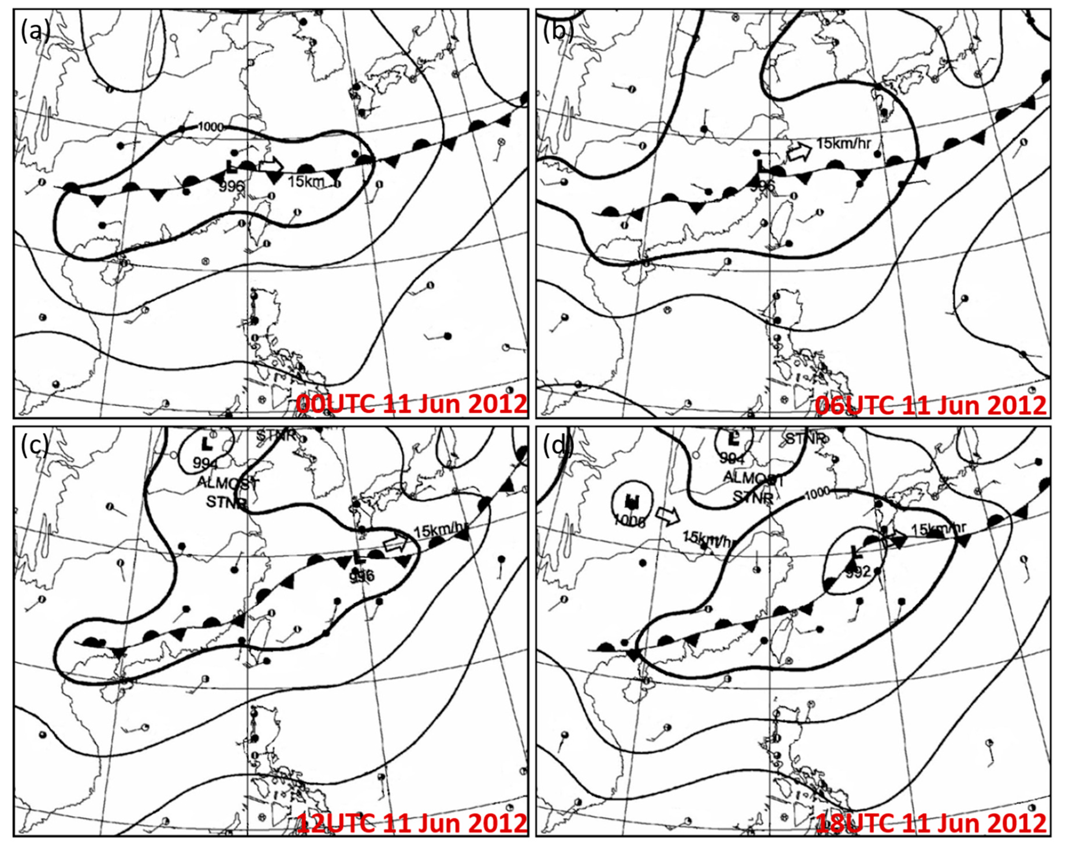
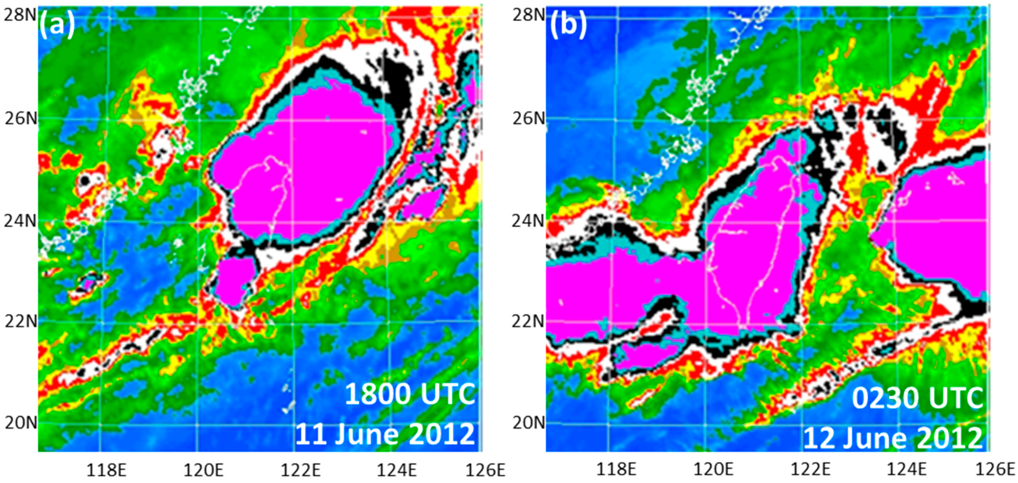
Figure 1 is a series of synoptic chart at surface (6-h interval) from 0000 UTC 11 June 2012 through 1800 UTC 11 June 2012. The stationary front was in parallel with latitudinal line in the vicinity of Taiwan northern ocean during the analysis period, in the NE-SW direction. The color-enhanced geostationary infrared 11-μm satellite imageries during the extreme precipitation stage are shown in
Figure 2. The pink color suggests a cold cloud-top feature which means multiple deep and matured mesoscale convection systems (MCSs) were developed within this front. These indicate the frontal system was quasi-stationary, and the whole Taiwan was exposed in a strong moisture and temperature gradients area. The whole system started to develop from 8 June 2012 in the southern China, and moved toward the east. In conjunction with the southwesterly moisture plume from the South China Sea and Bashi Channel, more than four major MCSs developed, matured and dissipated in this region till 14 June 2012. There were reports of six deaths, three missing, and sixteen injuries, and more than 1.5 million US dollars in economic lost were reported during this heavy precipitation case.
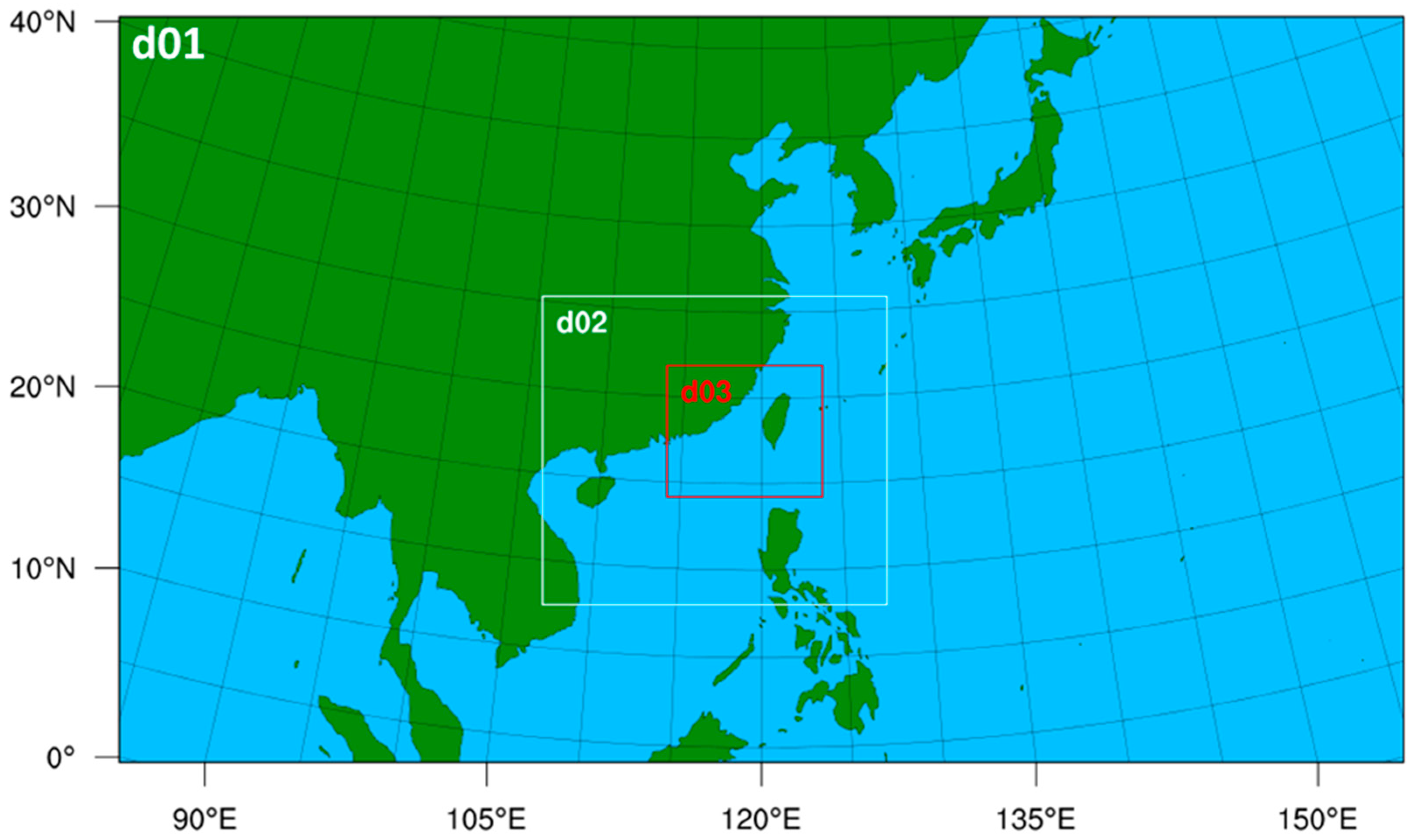
The WRF and WRF 3D-var systems were used to access the potential impact of two types of AIRS soundings data on the predicting the development of this heavy precipitation event. The model is compressible and nonhydrostatic, and thus it is sufficient to depict the frontal system with MCSs. We performed the simulation using a one-way nesting system with three model domains with spatial resolutions of 45 km, 15 km and 5 km, which are equivalent to 180 by 105, 145 by 130 and 196 by 166 horizontal grid points, respectively (
Figure 3). The outer model domain provided the initial and boundary conditions to the nested grid domain. In the vertical coordinate, the model top was set at 30 hPa with 30 terrain-following hydrostatic pressure levels. The model simulations employed the cloud microphysics scheme of the WRF single-moment 5-class (WSM5) and the cumulus parameterization of the modified version of the Kain–Fritsch scheme. The Yonsei University (YSU) scheme and Rapid Radiative Transfer Model (RRTM) longwave-Dudhia shortwave schemes were used for the PBL and atmospheric radiation process, respectively. The vertical layers and all model physics were the same in all domains, except the cumulus parameterization was turned off in the finest horizontal resolution domain (i.e., “d03” in
Figure 3).
Five experiments were conducted initially: (1) control (CTRL hereafter); (2) all SFOV soundings; (3) all SUP soundings; (4) cross-matched clear SFOV soundings; and (5) cross-matched clear SUP sounding, and are summarized in
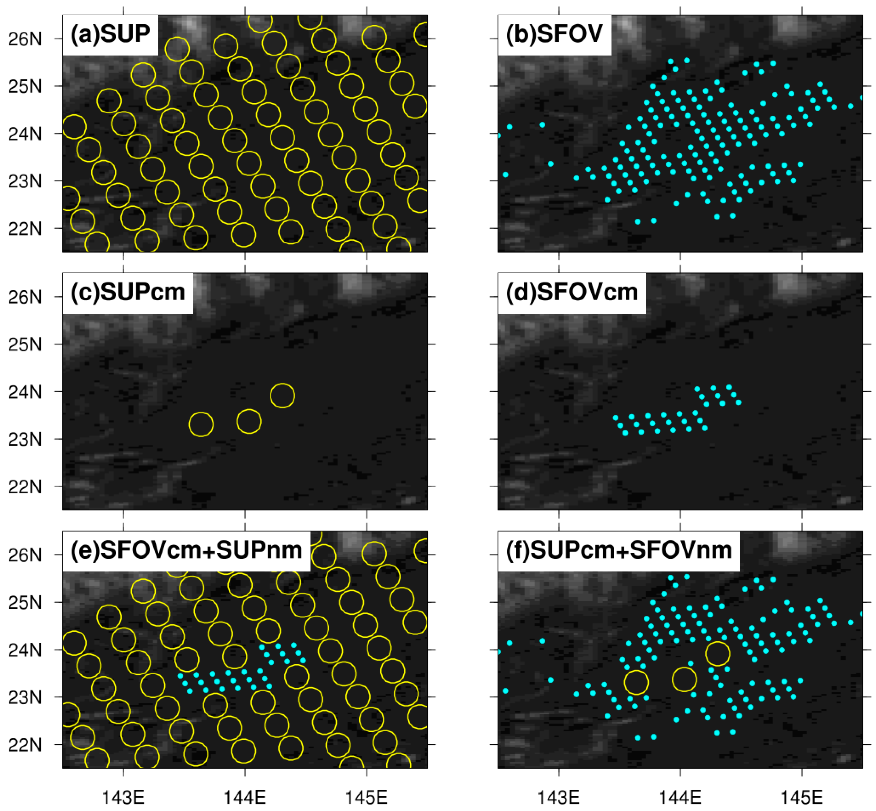
Table 1. The CTRL experiment assimilated the conventional measurements from the global telecommunication system (GTS). The second and third experiments are identical to the CTRL, except that all available SFOV and SUP retrievals were also assimilated through WRF 3D-var system. Since two types of soundings may have different spatial coverage and retrieval uncertainties may vary in clear or cloudy scene in these three experiments, additional experiments were conducted to ensure the consistency of observation constraints. We cross matched both SFOV and SUP data and applied their individual stringent quality control as described previously. Only if nine AIRS SFOV soundings are categorized as clear scene within one AMSU footprint, the retrieved parameters from both SFOV and SUP systems are assimilated with the conventional observations as the “SFOVcm” and “SUPcm” experiments. These two experiments could ensure the spatial coverage from two types of soundings are comparable over clear skies. However, retrievals from SFOV soundings are supposed to retain better gradient information than SUP data due to its finer instrumental resolution. Schematic examples shown in
Figure 4a,b indicate experiments (2) and (3), respectively. The yellow circles and cyan dots in
Figure 4 depict the SUP and SFOV observations.
Figure 4c,d shows experiments (4) and (5), respectively. Additional experiments were performed to evaluate the optimal configurations (i.e.,
Figure 4e,f) and will be described in
Section 5 and summarized in
Table 2.
All assimilation experiments were performed with continuous cycling of a 6-h assimilation window in the outer domains (i.e., “d01” and “d02” in
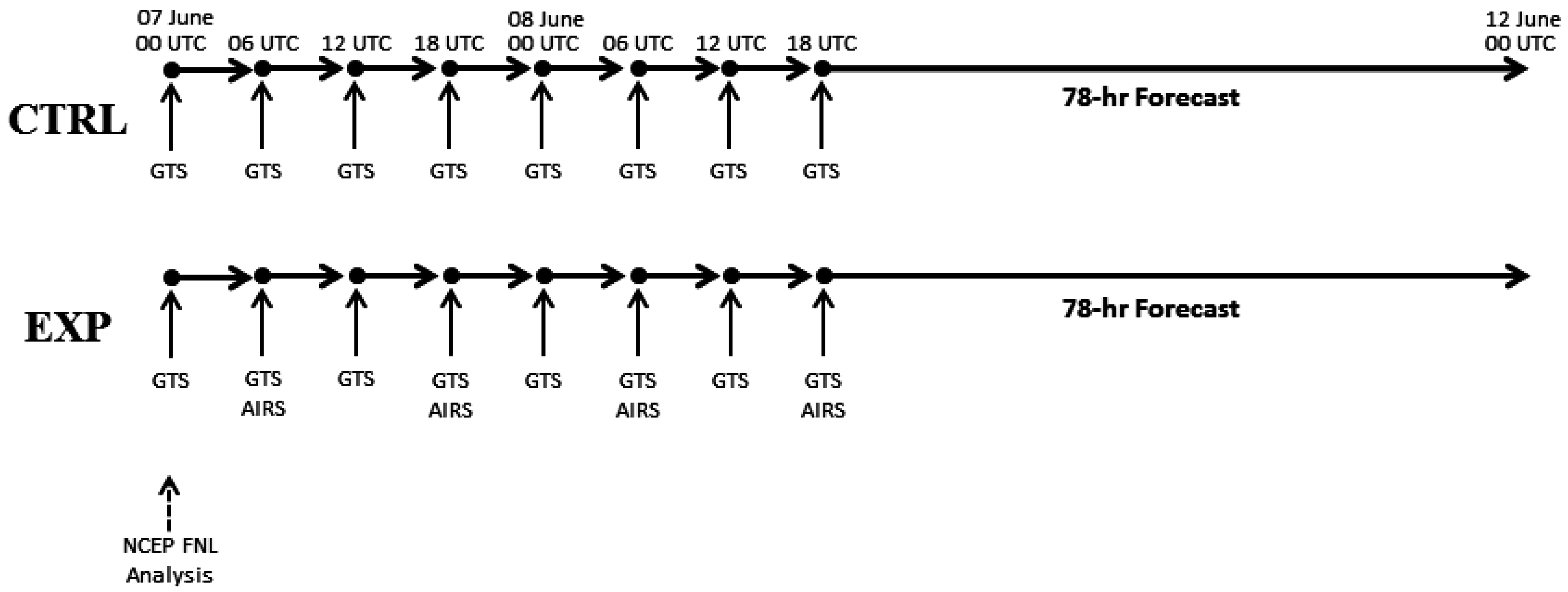
Figure 3), which could improve the predictability in the nested domains by providing a better synoptic-scale environment and forcing. For each cycle, the background fields were provided with a 6-h WRF forecast that had been initialized with the WRF 3D-var analysis. From the second cycle, the CTRL and SFOV/SUP experiments used different background fields resulting from the previous cycle of their own experiment. We performed continuous assimilation up to 42-h from 0000 UTC 7 June 2012 to 1800 UTC 8 June 2012, including a total of eight analysis-update cycles, then 78-h forecasts were produced from 1800 UTC 8 June 2012 to 0000 UTC 12 June 2012.
Figure 5 illustrates the schematic diagram of this experimental design. Identical assimilation and forecast strategy was repeated to perform the next run in the following day, i.e., 0000 UTC 9 June 2012. Each of the five experiments contains six independent runs of 42-h analysis-update and 78-h forecast fields. Therefore, we have the opportunity to investigate the impact of assimilating AIRS soundings on the forecast of the life cycle regarding this heavy frontal precipitation case.
4. Impact of AIRS Soundings on Heavy Frontal Precipitation Forecasts
4.1. Analysis with Two Types of Soundings Data Assimilation
During this heavy precipitation period, six individual simulations were performed by assimilating AIRS SFOV and SUP soundings along with CRTL experiments, as summarized in
Table 1. Our preliminary impact analysis is focused on the assessment of the following aspects. For every 6-h interval, the geopotential height, temperature, and mixing ratio at 300, 500, and 850 hPa were validated against the European Centre for Medium-Range Weather Forecasts (ECMWF) Reanalysis Interim (ERA-Interim) fields, which represent upper, middle and lower tropospheric atmosphere state. The root-mean-square difference (RMSD) and mean difference (MD) are calculated by using data from all the grid points in domain 2 for all the six runs. These are defined as follows:
where
and
are the ERA-Interim analysis and forecast fields, respectively.
is the number of the sample size within the comparison domain.
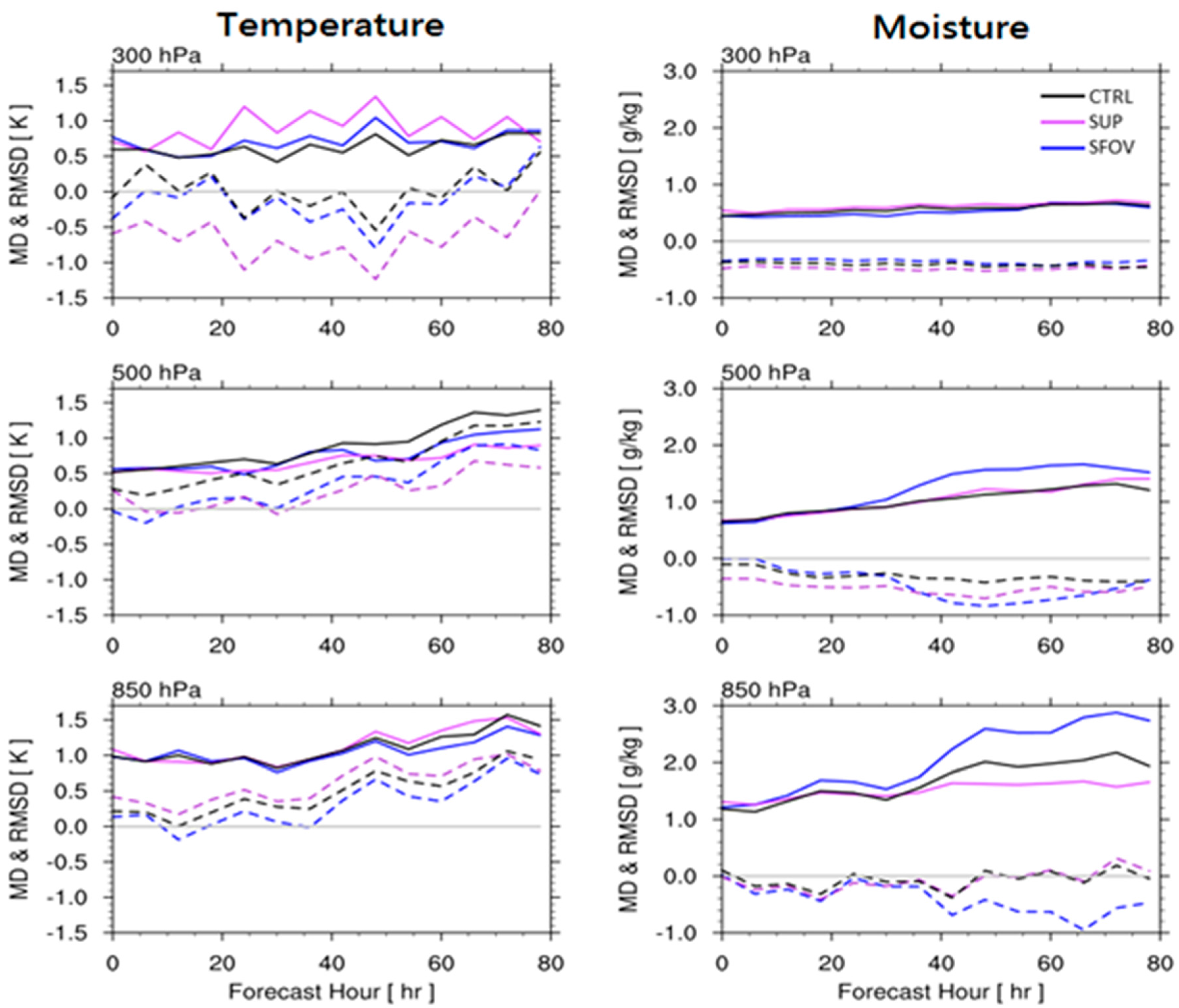
Figure 6 shows the RMSD (solid curves) and MD (dashed curves) of temperature and mixing ratio at 300 hPa, 500 hPa and 850 hPa for CTRL, SUP and SFOV experiments, respectively. The SUP experiment has improved predictability in 500 hPa temperature and moisture fields and 850 hPa moisture in terms of lower RMSD. On the other hand, SFOV has an advantage in temperature forecasts in both 300 and 850 hPa levels compared to SUP. This reveals the SUP data set has a positive contribution in moisture and SFOV data may benefit the temperature forecasts. One may have the concern that there are no consistencies between the temperature and moisture forecast skills because CTRL is sometimes better than one of the experiments. In order to have an overall evaluation of both temperature and moisture simultaneously, we analyzed the equivalent potential temperature (
), which is defined as
In Equation (3), is the temperature when the air parcel moves from the pressure level of to 1000 hPa (), is latent heat of evaporation in the unit of [kJ/kg], is specific heat at constant pressure for air in the unit of [J/(kg·K)], is moisture mixing ratio, and is specific gas constant.
The equivalent potential temperature contains the synergistic information from both temperature and moisture.
represents the moist state energy and has been used to evaluate the combined temperature and moisture states. Therefore, it may be served as an analogical parameter for two prognostic variables simultaneously [
38].
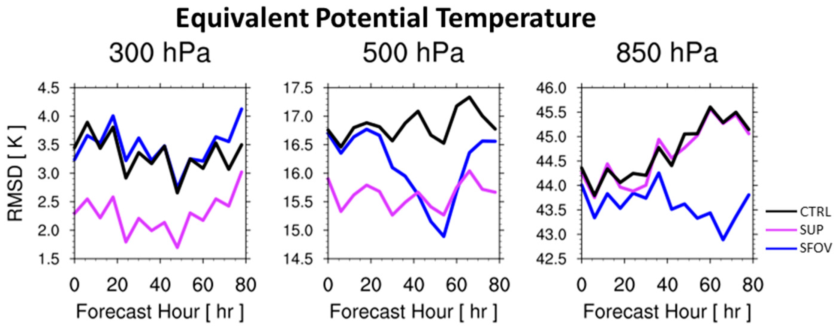
Figure 7 shows the RMSD of
at 300, 500 and 850 hPa levels, which indicates the SUP data will have positive impact in both upper and middle troposphere while SFOV does improve the lower troposphere throughout the forecast time.
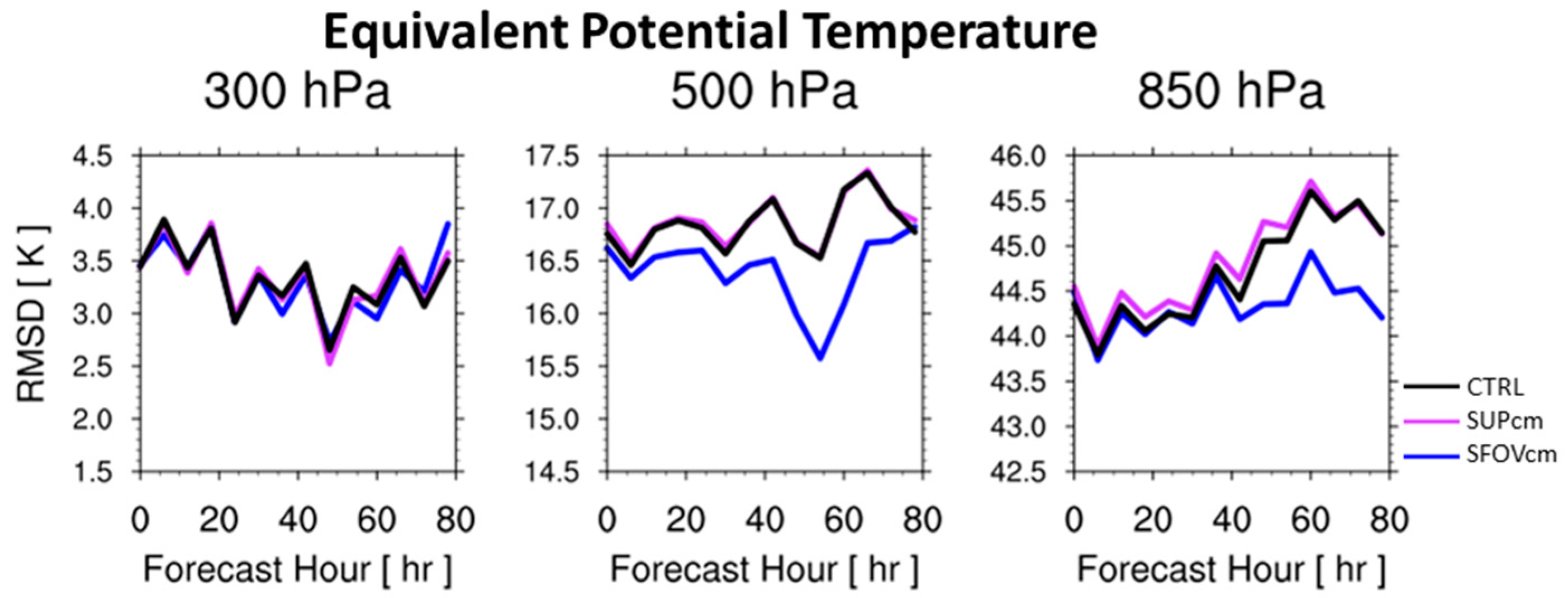
4.2. Analysis with Two Types of Soundings Assimilation at Matched Spatial Coverage
One may argue that the SFOV soundings contain an improved spatial resolution compared to SUP retrievals, but SFOV data set only benefits to the lower troposphere. Therefore, we re-examine the used SUP and SFOV data during the assimilation, and the different spatial coverage patterns are identified in the experiments. For SUP sounding, it covers a broader region than SFOV retrievals due to the primary SUP observation has the feature from microwave observation. Therefore, SUP soundings could cover the cloudy skies when cross checked with the 11-μm (window channel) brightness temperature imagery. On the other hand, SFOV retrievals are conducted in the clear skies so that there is limited coverage but higher spatial resolution than SUP data as described previously. Hence, we carried out similar experiments as in
Section 4.1 but only cross-matched SFOV and SUP data sets are used. There are nine (3 by 3) SFOV soundings within one SUP footprint typically. If these nine SFOVs are clear within one SUP footprint, we consider that they are cross-matched clear SFOV and SUP sounding as (4) SFOVcm and (5) SUPcm in
Table 1.
We compare the forecast performance between SFOVcm and SUPcm as shown in
Figure 8. The RMSD for equivalent potential temperature (
) indicated that SFOVcm has advantage over SUPcm, in particular at the 500 hPa level. The upper troposphere has about the same forecast capability in regard to a relative homogeneous atmospheric thermodynamic state so that spatial resolution issue in these altitudes is not that significant than in the lower troposphere. On the contrary, the 850 hPa does suggest that SFOVcm has better performance than SUPcm, especially in the forecasts after 40 h and beyond. This demonstrates the importance of higher spatial resolution soundings, and it could benefit the numerical weather forecast in the middle and lower troposphere, which is closely and directly related to human activities.
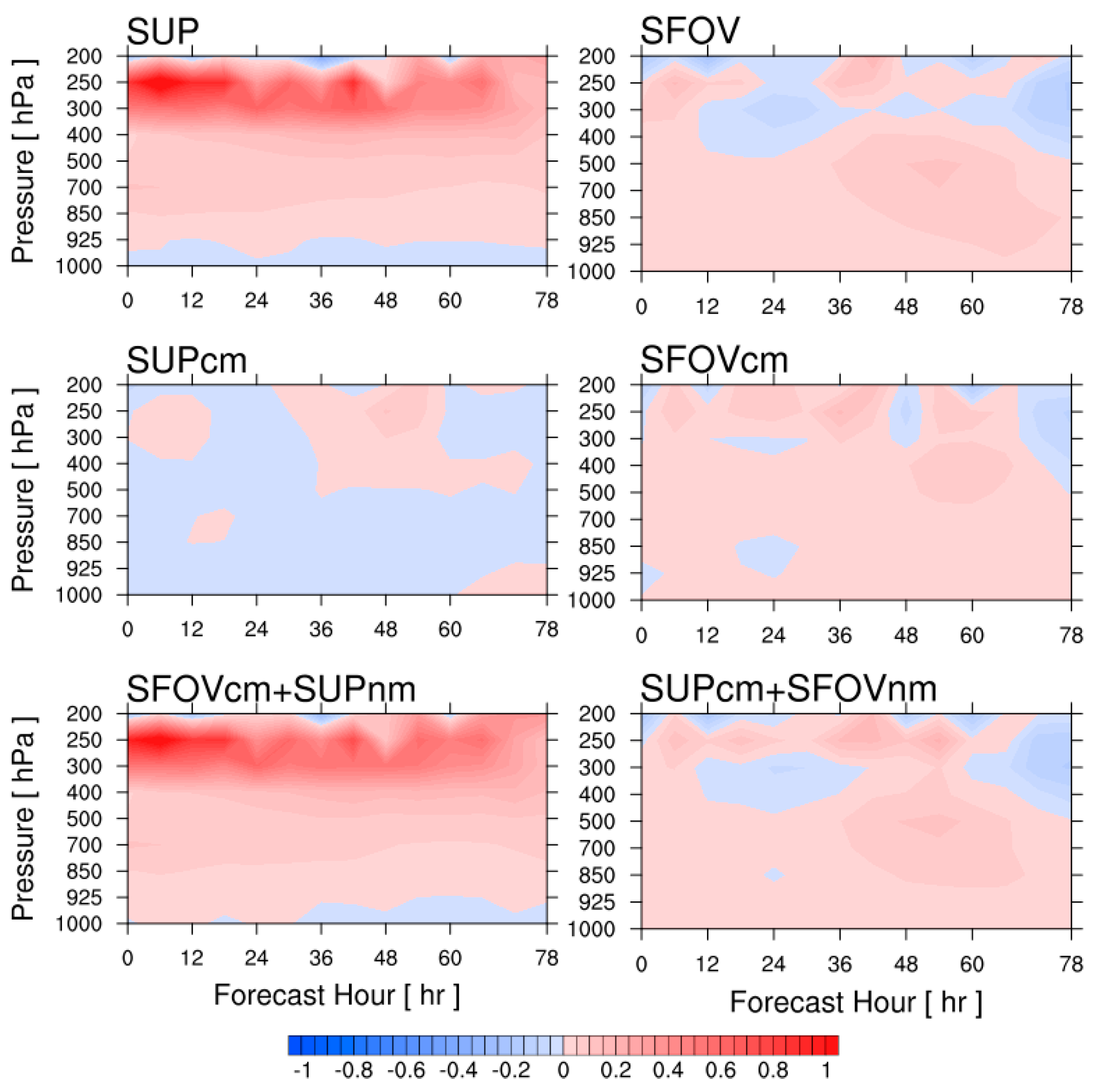
5. Optimal Use of SFOV and SUP Soundings Discussions
Based on the analysis and sensitivity tests between SFOV and SUP soundings in
Section 4, we proposed two additional experiments as shown in
Table 2 in order to suggest the best use of these two soundings. We intended to take advantage of them, such as the cloudy sounding and retaining the finer spatial resolution in some cases. We evaluated two extreme cases that the first one combines SUPcm and those not cross-matched individual SFOV as “SUPcm+SFOVnm”, and the second one uses SFOVcm in conjunction with not cross-matched SUPcm as “SFOVcm+SUPnm”. Both represent the meaning that retains cross-match feature with the assist from not cross-matched observations.
We defined an index to evaluate the forecast impact (
) as follows:
where
and
are RMSD of the analyzed variable for control (configuration (1) in
Table 1) and additional experiments (configurations (2) to (7) in
Table 1 and
Table 2), respectively. Positive
values indicate better forecast than the control run, and vice versa.
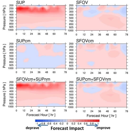
Figure 9 is the
for all experiments in
Section 4 (
Table 1) along with the proposed optimal combinations (
Table 2) on equivalent potential temperature. One may notice that SUP soundings have largest positive feedback in the upper portion of troposphere (pressure levels between 200 to 400 hPa in the top left panel of
Figure 9) while SFOV soundings have positive impacts on the pressure levels between 400 to 1000 hPa, in particular of 36 to 72 h forecasts (middle left panel of
Figure 9). The SUPcm is not significant as SUP experiment, which may be due to reduced amount of data assimilated in the initial and boundary fields (top right panel of
Figure 9). The SFOVcm continues to have a positive impact in the middle to lower troposphere after 36 h but with a smaller
for the same reason as the SFOVcm case.
Note that the two proposed optimal experiments are in the bottom left and right panels in
Figure 9. We see “SFOVcm+SUPnm” retains the successful performance from SUP, and hold positive impacts throughout the whole levels from boundary layer to the upper troposphere. On the contrary, “SUPcm+SFOVnm” experiment (bottom right panel) retained the
from SFOV experiment but not as promising as “SFOVcm+SUPnm” in the bottom left panel. Hence, we suggest the “SFOVcm+SUPnm” is the best optimal combination for the NWP forecast because SFOVcm keeps the atmospheric gradient and SUPnm provides the critical information in the cloudy scenes. With this configuration, we have the capability to conduct the best forecast performance in the layered troposphere throughout this heavy precipitation case.
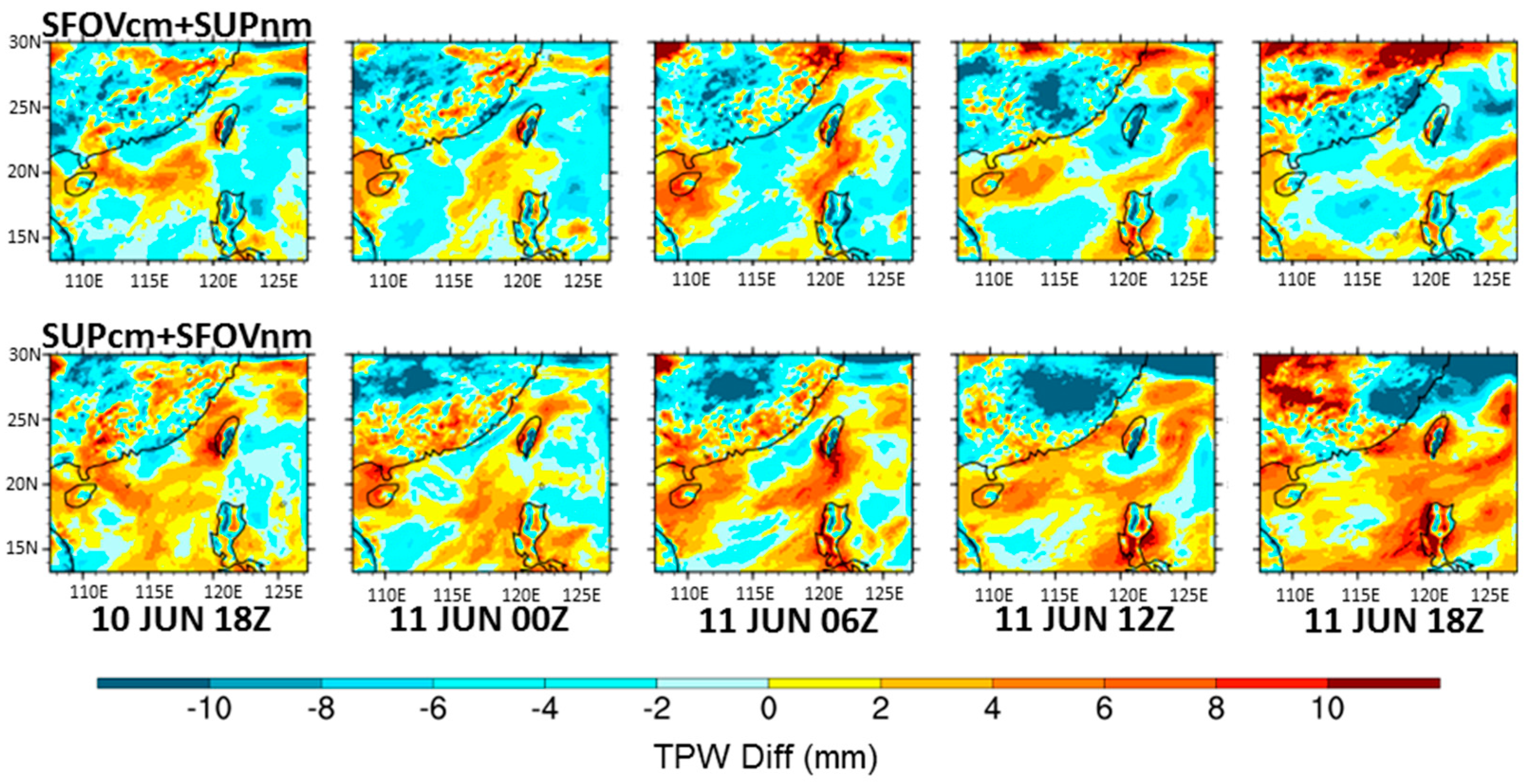
One may have interest in the total precipitable water (TPW) forecast skill,
Figure 10 reveals the TPW difference away from ERA-Interim fields. These are the 24-h forecasts from 1800 UTC 10 June 2012 for “SFOVcm+SUPnm” and “SUPcm+SFOVnm” experiments to 1800 UTC 11 June 2012. Warm (cold) colors suggest the forecasted TPW are more (less) than ERA-Interim. It is obvious that “SFOVcm+SUPnm” experiment has lower TPW forecasts than “SUPcm+SFOVnm” at the analysis time of 1800 UTC on 10 June 2012 in the “d02” of
Figure 3. In the following 6-h through 24-h forecasts, upper panels generally have advantage over bottom panels, which confirms the optimal use of clear-sky matched IR retrievals with non-matched MW soundings (i.e., “SFOVcm+SUPnm”) is a proper choice because of less TPW difference when compared to ERA-Interim data set.
6. Discussion
In order to investigate the impact due to the observational and retrieval uncertainties in the numerical weather prediction model, we performed a series of experiments to seek the possibility of their optimal use. We used a 3D-var based data assimilation technique to incorporate the conventional observations data and space-born hyperspectral infrared (IR; SFOV) and microwave (MW; SUP) soundings so that the initial and boundary conditions could be revised accordingly in this NWP forecast system. A heavy precipitation case in Taiwan vicinity, which is associated with Mei-Yu frontal system in June 2012, is used for the study. Simulations of 78-h forecasts with various combinations of IR and MW data sets are conducted over six days, which cover the whole cycle of the heavy precipitation system.
The initial result shows that both IR and MW could benefit the NWP system forecast capability in different parts of the atmospheric levels. The MW soundings, which have coarser spatial resolution, could improve the moisture forecast in the middle (500 hPa) and lower (850 hPa) troposphere, and also promote the performance of temperature forecast in the middle troposphere. The fine spatial resolution of IR retrievals improves the temperature forecast in the upper (300 hPa) and lower troposphere.
The discrepancy in spatial coverages for IR and MW sounding data sets are addressed in this study. Because the IR and MW soundings are available in different locations, cross-matched experiments are carried out to evaluate the relative importance on both retrievals so that we could ensure both data sets are in the same spatial coverage. We could see the IR sounding has advantage to improve the forecast than MW data because of the retention of a better atmospheric horizontal gradient.
7. Conclusions
In this study, we attempt to determine the optimal utilization of both IR and MW soundings for the NWP system. We find that SFOVcm with non cross-matched SUP (SUPnm) data sets synergistically used has greatly improved the forecast performance compared to either data set alone in the tropospheric atmosphere. The upper part of troposphere (200 to 400 hPa) could be better forecasted by the support of MW retrievals, while IR sounding facilitates the middle and lower part of the troposphere.
We intend to allocate the uncertainty in the forecast system from IR and MW retrievals and propose the optimal use of two soundings simultaneously. The statistics of forecast performance demonstrated that their synergistic use is feasible. Future works may include the various degree of retrieval system performance, and the length and frequency of cycling window, since these may affect the initial and boundary conditions through data assimilation technique.
Acknowledgments
The authors would like to thank the NASA AIRS Science Team to provide the AIRS/AMSU (SUP) sounding data set, and the University of Wisconsin-CIMSS for assisting some initial question on the AIRS CHISR algorithm (SFOV). This work was supported by multiple projects from Taiwan’s Ministry of Science and Technology (Grants MOST 104-2119-M-008-009, MOST 104-2625-M-008-003, MOST 105-2923-M-008-001-MY3, MOST 105-2625-M-008-010, and MOST 105-2119-M-008-011).
Author Contributions
C.-Y.L. is the primary author who established the concept of the presented study. C.-Y.L. performed the assimilation of both hyperspectral IR and MW soundings in the NWP model. S.-C.K., A.H.N.L., S.-C.H. and Y.-C.Y. assisted the model evaluation and statistics. K.-H.T. and N.-C.Y. addressed the assessment of ECMWF reanalysis, and some figures plotting in the study.
Conflicts of Interest
The authors declare no conflict of interest.
References
- Singh, R.; Kishtawal, C.M.; Ojha, S.P.; Pal, P.K. Impact of assimilation of Atmospheric InfraRed Sounder (AIRS) radiances and retrievals in the WRF 3D-Var assimilation system. J. Geophys. Res. 2012, 117. [Google Scholar] [CrossRef]
- Pu, Z.; Zhang, L. Validation of Atmospheric Infrared Sounder temperature and moisture profiles over tropical oceans and their impact on numerical simulations of tropical cyclones. J. Geophys. Res. Atmos. 2010, 115, 9–12. [Google Scholar] [CrossRef]
- Chien, F.C.; Kuo, Y.-H. Impact of FORMOSAT-3/COSMIC GPS radio occultation and dropwindsonde data on regional model predictions during the 2007 Mei-yu season. GPS Solut. 2010, 14, 51–63. [Google Scholar] [CrossRef]
- Lorenc, A.C.; Ballard, S.P.; Bell, R.S.; Ingleby, N.B.; Andrews, P.L.F.; Barker, D.M.; Bray, J.R.; Clayton, A.M.; Dalby, T.; Li, D.; et al. The Met Office global three-dimensional variational data assimilation scheme. Q. J. R. Meteorol. Soc. 2000, 126, 2991–3012. [Google Scholar] [CrossRef]
- Le Marshall, J.; Jung, J.; Derber, J.; Chahine, M.; Treadon, R.; Lord, S.J.; Woollen, J. Improving global analysis and forecasting with AIRS. Bull. Am. Meteorol. Soc. 2016, 87, 891–894. [Google Scholar] [CrossRef]
- Migliorini, S. On the equivalence between radiance and retrieval assimilation. Mon. Weather Rev. 2012, 140, 258–265. [Google Scholar] [CrossRef]
- Zavodsky, B.T.; Chou, S.-H.; Jedlovec, G.; Lapenta, W. The impact of Atmospheric Infrared Sounder (AIRS) profiles on short-term weather forecasts. Proc. SPIE 2007, 6565. [Google Scholar] [CrossRef]
- Li, J.; Liu, H. Improved hurricane track and intensity forecast using single field-of-view advanced IR sounding measurements. Geophys. Res. Lett. 2009, 36. [Google Scholar] [CrossRef]
- Pagano, T.S.; Aumann, H.H.; Hagan, D.E.; Overoye, K. Prelaunch and in-flight radiometric calibration of the Atmospheric Infrared Sounder (AIRS). IEEE Trans. Geosci. Remote Sens. 2003, 41, 265–273. [Google Scholar] [CrossRef]
- Lambrigtsen, B.H.; Lee, S.Y. Coalignment and synchronization of the AIRS instrument suite. IEEE Trans. Geosci. Remote Sens. 2003, 41, 343–351. [Google Scholar] [CrossRef]
- Chahine, M.T.; Pagano, T.S.; Aumann, H.H.; Atlas, R.; Barnet, C.; Blaisdell, J.; Gautier, C. AIRS: Improving weather forecasting and providing new data on greenhouse gases. Bull. Am. Meteorol. Soc. 2006, 87, 911–926. [Google Scholar] [CrossRef]
- Tobin, D.C.; Revercomb, H.E.; Knuteson, R.O.; Lesht, B.M.; Strow, L.L.; Hannon, S.E.; Cress, T.S. Atmospheric Radiation Measurement site atmospheric state best estimates for Atmospheric Infrared Sounder temperature and water vapor retrieval validation. J. Geophys. Res. Atmos. 2006, 111. [Google Scholar] [CrossRef]
- Susskind, J.; Blaisdell, J.; Iredell, L. Significant advances in the AIRS Science Team Version-6 retrieval algorithm. Proc. SPIE 2012. [Google Scholar] [CrossRef]
- McCarty, W.; Jedlovec, G.; Miller, T.L. Impact of the assimilation of Atmospheric Infrared Sounder radiance measurements on short-term weather forecasts. J. Geophys. Res. 2009, 114. [Google Scholar] [CrossRef]
- Lim, A.H.; Jung, J.A.; Huang, H.L.A.; Ackerman, S.A.; Otkin, J.A. Assimilation of clear sky Atmospheric Infrared Sounder radiances in short-term regional forecasts using community models. J. Appl. Remote Sens. 2014, 8, 083655. [Google Scholar] [CrossRef]
- Atlas, R. The impact of AIRS data on weather prediction. Proc. SPIE 2005. [Google Scholar] [CrossRef]
- Jedlovec, G.J.; Chou, S.H.; Zavodsky, B.T.; Lapenta, W. The use of error estimates with AIRS profiles to improveshort-term weather forecasts. Proc. SPIE 2006. [Google Scholar] [CrossRef]
- Zheng, J.; Li, J.; Schmit, T.J.; Li, J.L.; Liu, Z.Q. The impact of AIRS atmospheric temperature and moisture profiles on hurricane forecasts: Ike and Irene. Adv. Atmos. Sci. 2015, 32, 319–335. [Google Scholar] [CrossRef]
- Li, J.; Huang, H.L. Retrieval of atmospheric profiles from satellite sounder measurements by use of the discrepancy principle. Appl. Opt. 1999, 38, 916–923. [Google Scholar] [CrossRef] [PubMed]
- Li, J.; Wolf, W.; Menzel, W.P.; Zhang, W.; Huang, H.-L.; Achtor, T.H. Global soundings of the atmosphere from ATOVS measurements: The algorithm and validation. J. Appl. Meteorol. 2000, 39, 1248–1268. [Google Scholar] [CrossRef]
- Weisz, E.; Huang, H.L.; Li, J.; Borbas, E.; Baggett, K.; Thapliyal, P.; Guan, L. International MODIS and AIRS processing package: AIRS products and applications. J. Appl. Remote Sens. 2007, 1, 013519. [Google Scholar] [CrossRef]
- Liu, C.-Y.; Li, J.; Weisz, E.; Schmit, T.J.; Ackerman, S.A.; Huang, H.L. Synergistic use of AIRS and MODIS radiance measurements for atmospheric profiling. Geophys. Res. Lett. 2008, 35. [Google Scholar] [CrossRef]
- Strow, L.L.; Hannon, S.E.; Souza-Machado, D.; Motteler, H.E.; Tobin, D. An overview of the AIRS radiative transfer model. IEEE Trans. Geosci. Remote Sens. 2003, 41, 303–313. [Google Scholar] [CrossRef]
- Li, J.; Huang, H.-L.; Liu, C.-Y.; Yang, P.; Schmit, T.J.; Wei, H.; Weisz, E.; Guan, L.; Menzel, W.P. Retrieval of Cloud Microphysical Properties from MODIS and AIRS. J. Appl. Meteorol. 2005, 44, 1526–1543. [Google Scholar] [CrossRef]
- Li, J.; Liu, C.-Y.; Huang, H.L.; Schmit, T.J.; Wu, X.; Menzel, W.P.; Gurka, J.J. Optimal cloud-clearing for AIRS radiances using MODIS. IEEE Trans. Geosci. Remote Sens. 2005, 43, 1266–1278. [Google Scholar]
- Li, J.; Liu, C.-Y.; Zhang, P.; Schmit, T.J. Applications of full spatial resolution space-based advanced infrared soundings in the preconvection environment. Weather Forecast. 2012, 27, 515–524. [Google Scholar] [CrossRef]
- Kwon, E.H.; Li, J.; Li, J.; Sohn, B.J.; Weisz, E. Use of total precipitable water classification of a priori error and quality control in atmospheric temperature and water vapor sounding retrieval. Adv. Atmos. Sci. 2012, 29, 263–273. [Google Scholar] [CrossRef]
- Liu, C.-Y.; Liu, G.-R.; Lin, T.-H.; Liu, C.-C.; Ren, H.; Young, C.-C. Using surface stations to improve sounding retrievals from hyperspectral infrared instruments. IEEE Trans. Geosci. Remote Sens. 2014, 52, 6957–6963. [Google Scholar]
- Liu, C.-Y.; Li, J.; Ho, S.-P.; Liu, G.-R.; Lin, T.-H.; Young, C.-C. Retrieval of Atmospheric Thermodynamic State from Synergistic Use of Radio Occultation and Hyperspectral Infrared Radiances Observations. IEEE J. Sel. Top. Appl. Earth Obs. Remote Sens. 2016, 9, 744–756. [Google Scholar] [CrossRef]
- Goldberg, M.D.; Qu, Y.; McMillin, L.M.; Wolf, W.; Zhou, L.; Divakarla, M. AIRS near-real-time products and algorithms in support of operational numerical weather prediction. IEEE Trans. Geosci. Remote Sens. 2003, 41, 379–389. [Google Scholar] [CrossRef]
- Susskind, J.; Barnet, C.; Blaisdell, J. Retrieval of atmospheric and surface parameters from AIRS/AMSU/HSB data in the presence of clouds. IEEE Trans. Geosci. Remote Sens. 2003, 41, 390–409. [Google Scholar] [CrossRef]
- Miyoshi, T.; Kunii, M. The Local Ensemble Transform Kalman Filter with the Weather Research and Forecasting Model: Experiments with Real Observations. Pure Appl. Geophys. 2012, 169, 321–333. [Google Scholar] [CrossRef]
- Kang, H.-J.; Yoo, J.-M.; Jeong, M.J.; Won, Y.-I. Uncertainties of satellite-derived surface skin temperatures in the polar oveans: MODIS, AIRS/AMSU, and AIRS only. Atmos. Meas. Tech. 2015, 8, 4025–4041. [Google Scholar] [CrossRef]
- Skamarock, W.C.; Klemp, J.B.; Duhia, J.; Gill, D.O.; Barker, D.M.; Duda, M.G.; Huang, X.-Y.; Wang, W.; Powers, J.G. A description of the Advanced Research WRF Version 3. Available online: http://opensky.ucar.edu/islandora/object/technotes:500 (accessed on 30 March 2016).
- Barker, D.; Huang, X.-Y.; Liu, Z.; Auligne, T.; Zhang, X.; Rugg, S.; Ajjaji, R.; Bourgeois, A.; Bray, J.; Chen, Y.; et al. The weather research and forecasting model’s community variational/ensemble data assimilation system: WRFDA. Bull. Am. Meteorol. Soc. 2012, 93, 831–843. [Google Scholar] [CrossRef]
- Barker, D.M.; Huang, W.; Guo, Y.; Bourgeois, A.J.; Xiao, Q.N. A Three-Dimensional Variational Data Assimilation System for MM5: Implementation and Initial Results. Mon. Weather Rev. 2004, 23, 897–914. [Google Scholar] [CrossRef]
- Parrish, D.F.; Derber, J.C. The National Meteorological Center’s spectral-interpolation analysis system. Mon. Weather Rev. 1992, 120, 1747–1763. [Google Scholar] [CrossRef]
- Davies-Jones, R. On formulas for equivalent potential temperature. Mon. Weather Rev. 2009, 137, 3137–3148. [Google Scholar] [CrossRef]
Figure 1.
Synoptic charts of Mei-Yu frontal system at: (a) 0000 UTC; (b) 0600 UTC; (c) 1200 UTC; and (d) 1800 UTC on 11 June 2012. The quasi-stationary frontal system was between Korean peninsula and Taiwan on this day, and gradually moved toward the northern Taiwan.
Figure 1.
Synoptic charts of Mei-Yu frontal system at: (a) 0000 UTC; (b) 0600 UTC; (c) 1200 UTC; and (d) 1800 UTC on 11 June 2012. The quasi-stationary frontal system was between Korean peninsula and Taiwan on this day, and gradually moved toward the northern Taiwan.
Figure 2.
The color enhanced Japanese geostationary satellite (MTSAT-2) window channel brightness temperature imagery at wavelength of 11-μm: (a) 1800 UTC on 11 June 2012; and (b) 0230 UTC on 12 June 2012. The pink color indicates the cloud tops with deep convection, which are typically associated with heavy precipitation at the surface.
Figure 3.
The three nested domains (d01, d02, and d03) in the NWP model experiment in this study. The spatial resolutions and horizontal grids of these three domains are 45-, 15-, and 5-km (or 180 by 105, 145 by 130, and 196 by 166), respectively.
Figure 3.
The three nested domains (d01, d02, and d03) in the NWP model experiment in this study. The spatial resolutions and horizontal grids of these three domains are 45-, 15-, and 5-km (or 180 by 105, 145 by 130, and 196 by 166), respectively.
Figure 4.
The conceptual sounding data spatial distribution for the experiments in the study: (
a,
b) “SUP” and “SFOV”; (
c,
d) “SUPcm” and “SFOVcm”); and (
e,
f) “SFOVcm+SUPnm” and “SUPcm+SFOVnm”. See
Table 1 and
Table 2 for the detail cross-matched (cm) and non-matched (nm) descriptions.
Figure 4.
The conceptual sounding data spatial distribution for the experiments in the study: (
a,
b) “SUP” and “SFOV”; (
c,
d) “SUPcm” and “SFOVcm”); and (
e,
f) “SFOVcm+SUPnm” and “SUPcm+SFOVnm”. See
Table 1 and
Table 2 for the detail cross-matched (cm) and non-matched (nm) descriptions.
Figure 5.
Schematic diagram of the experimental design illustrating an example data assimilation cycle and the 78-h forecast from 1800 UTC 8 June 2012.
Figure 5.
Schematic diagram of the experimental design illustrating an example data assimilation cycle and the 78-h forecast from 1800 UTC 8 June 2012.
Figure 6.
Statistics of forecast performance of temperature (left column) and moisture (right column) at 300 (top row), 500 (middle row) and 850 hPa (bottom row) on CTRL (black curves), SUP (purple curves) and SFOV (blue curves) experiments. The solid curves are RMSD, and the dashed curves are MD.
Figure 6.
Statistics of forecast performance of temperature (left column) and moisture (right column) at 300 (top row), 500 (middle row) and 850 hPa (bottom row) on CTRL (black curves), SUP (purple curves) and SFOV (blue curves) experiments. The solid curves are RMSD, and the dashed curves are MD.
Figure 7.
Statistics of the forecast performance of equivalent potential temperature at 300 (left panel), 500 (middle panel) and 850 (right panel) hPa pressure levels for CTRL (black curves), SUP (purple curves) and SFOV (blue curves) experiments.
Figure 7.
Statistics of the forecast performance of equivalent potential temperature at 300 (left panel), 500 (middle panel) and 850 (right panel) hPa pressure levels for CTRL (black curves), SUP (purple curves) and SFOV (blue curves) experiments.
Figure 8.
Statistics of the forecast performance of equivalent potential temperature at 300 (left panel), 500 (middle panel) and 850 (right panel) hPa pressure levels for CTRL (black curves), SUPcm (purple curves) and SFOVcm (blue curves) experiments.
Figure 8.
Statistics of the forecast performance of equivalent potential temperature at 300 (left panel), 500 (middle panel) and 850 (right panel) hPa pressure levels for CTRL (black curves), SUPcm (purple curves) and SFOVcm (blue curves) experiments.
Figure 9.
The forecast impact (
) of the individual experiments in
Table 1 and
Table 2. Warm (cold) colors suggest a positive (negative) contribution to the forecast system when compared to the control run.
Figure 9.
The forecast impact (
) of the individual experiments in
Table 1 and
Table 2. Warm (cold) colors suggest a positive (negative) contribution to the forecast system when compared to the control run.
Figure 10.
The 24-h forecasts total precipitable water (TPW) against ERA-Interim fields from 1800 UTC 10 June 2012 to 1800 UTC 11 June 2012 (from left to right columns: at 0-h analysis time, and 6-, 12-, 18-, and 24-h forecasts). The upper row is the TPW difference between “SFOVcm+SUPnm” and ERA-Interim fields. The bottom row is the TPW difference between “SUPcm+SFOVnm” and ERA-Interim fields.
Table 1.
The summary of numerical experiments in this study. The designed experiments are abbreviated in the left column, and assimilated observations are listed in the right column. Note that nine (3 by 3) clear SFOV soundings within one SUP footprint are considered as “cross-matched” in both SFOVcm and SUPcm experiments.
| Experiment | Assimilated Observations |
|---|
| (1) CTRL | GTS only |
| (2) SFOV | GTS, all available SFOV soundings |
| (3) SUP | GTS, all available SUP soundings |
| (4) SFOVcm | GTS, cross-matched clear SFOV soundings |
| (5) SUPcm | GTS, cross-matched clear SUP soundings |
Table 2.
The configuration of numerical experiments for optimal evaluation of the IR and MW soundings. The designed experiments are abbreviated in the left column, and assimilated observations are listed in the right column.
Table 2.
The configuration of numerical experiments for optimal evaluation of the IR and MW soundings. The designed experiments are abbreviated in the left column, and assimilated observations are listed in the right column.
| Experiment | Assimilated Observations |
|---|
| (6) SUPcm+SFOVnm | GTS, SUPcm with SFOV non-matched |
| (7) SFOVcm+SUPnm | GTS, SFOVcm with SUP non-matched |
© 2016 by the authors; licensee MDPI, Basel, Switzerland. This article is an open access article distributed under the terms and conditions of the Creative Commons Attribution (CC-BY) license (http://creativecommons.org/licenses/by/4.0/).


 ,
, 


