Mapping Daily Air Temperature for Antarctica Based on MODIS LST

Abstract

Spatial predictions of near-surface air temperature ($T_{air}$) in Antarctica are required as baseline information for a variety of research disciplines. Since the network of weather stations in Antarctica is sparse, remote sensing methods have large potential due to their capabilities and accessibility. Based on the MODIS land surface temperature (LST) data, $T_{air}$ at the exact time of satellite overpass was modelled at a spatial resolution of 1 km using data from 32 weather stations. The performance of a simple linear regression model to predict $T_{air}$ from LST was compared to the performance of three machine learning algorithms: Random Forest (RF), generalized boosted regression models (GBM) and Cubist. In addition to LST, auxiliary predictor variables were tested in these models. Their relevance was evaluated by a Cubist-based forward feature selection in conjunction with leave-one-station-out cross-validation to reduce the impact of spatial overfitting. GBM performed best to predict $T_{air}$ using LST and the month of the year as predictor variables. Using the trained model, $T_{air}$ could be estimated with a leave-one-station-out cross-validated $R^2$ of 0.71 and a RMSE of 10.51 ${}^{\circ }$C. However, the machine learning approaches only slightly outperformed the simple linear estimation of $T_{air}$ from LST ($R^2$ of 0.64, RMSE of 11.02 ${}^{\circ }$C). Using the trained model allowed creating time series of $T_{air}$ over Antarctica for 2013. Extending the training data by including more years will allow developing time series of $T_{air}$ from 2000 on.

1. Introduction

Near-surface air temperature ($T_{air}$) plays an important role in ecological, glaciological and climatological processes in Antarctica. Climate change further raises the need to study the spatio-temporal trends in $T_{air}$ and its induced regional feedback processes. Therefore, spatially explicit $T_{air}$ datasets are of high interest for the scientific community and research effort for its construction is in high demand [1].

A common approach to obtain spatially explicit $T_{air}$ datasets is spatial interpolation based on station records [2,3,4,5]. However, interpolation methods rely on a sufficiently dense number of points. Due to the remoteness of Antarctica, the network of weather stations is sparse [6] which makes simple interpolation approaches difficult. The applications of these methods to Antarctica are therefore limited to a low temporal resolution of e.g. annual means [7], rather than aiming at daily products. In order to obtain medium resolution datasets of $T_{air}$, remote sensing is a promising alternative: it offers spatially explicit proxies for $T_{air}$, and is therefore suitable for areas with low weather station density, such as Antarctica [8]. Though $T_{air}$ cannot be directly measured from space, land surface temperature (LST) is a widely used derived product from infrared bands and a proxy for $T_{air}$ [9] due to surface-atmosphere energy exchange processes.

The Moderate Resolution Imaging Spectroradiometer (MODIS) sensor onboard the Terra and Aqua spacecrafts acquires LST data four times per day (two during the day, two during the night) with a spatial resolution of 1km. MODIS LST was successfully used to estimate $T_{air}$ for various regions of the world [10,11,12,13,14,15,16,17]. Kilibarda et al. [18] performed a kriging based spatio-temporal interpolation of global daily temperatures including MODIS LST as predictor. However, since the focus of this study was on a global $T_{air}$ prediction, Antarctica was only marginally represented in the training data. Applications of MODIS LST to predict $T_{air}$ for Antarctica are limited to the study of Wang et al. [19] who compared monthly averages of MODIS LST with $T_{air}$ in the Lambert Glacier Basin in East Antarctica.

The majority of the studies rely on linear regressions or simple bias corrections to estimate $T_{air}$ from LST alone. However, the linearity of the relation is questionable. Colombi et al. [11] found differences in the performance of the linear model according to daytime and altitude. Vancutsem et al. [10] noticed variations in the performance depending on region and season, while Benali et al. [15] used several predictors and tested different model structures which included auxiliary predictors. Also Xu et al. [20] included land cover type and altitude in their models to improve the simple linear model between LST and $T_{air}$. Most recently, Janatian et al. [21] tested the importance of 11 auxiliary variables in addition to LST in a stepwise regression analysis and revealed julian day, altitude and solar zenith angle as effective additional predictors for $T_{air}$. Emamifar et al. [22] used M5 regression trees to model daily $T_{air}$ in Iran from MODIS LST and auxiliary variables and highlighted the advantage of tree-based models for an operational monitoring of $T_{air}$. Surprisingly, machine learning algorithms were only rarely applied in the context of estimating $T_{air}$ using LST [22,23]. However, those methods are good contenders to model $T_{air}$, since they can handle non-linearity and highly correlated predictor variables [24,25].

The aim of this study is to create a medium resolution spatially explicit daily $T_{air}$ product for Antarctica. In this context, we have tested the performance of different machine learning algorithms to estimate $T_{air}$ from LST and auxiliary variables as an alternative to a simple linear approach.

2. Methods

2.1. Data and Preprocessing

2.1.1. MODIS LST

The daily LST data (version 5 [26]) based on the MODIS sensor onboard the Aqua and Terra satellites are distributed as the MOD11A1 and MYD11A1 products [27]. The MODIS LST products consist of daytime and nighttime measurements at 1 km resolution. Their calculation is based on a split-window algorithm that uses the emissivities from MODIS bands 31 and 32 that were, in turn, calculated using information about land cover type, atmospheric column water vapour and lower boundary air surface [26]. The data are cloud-masked on the basis of the MODIS Cloud Mask algorithm [28] that applies typical thresholds in the visible and infrared channels. The MODIS LST data are stated to be very accurate with a deviation of mostly below 1K in the range between −10 ${}^{\circ }$C and 58 ${}^{\circ }$C [26]. Regarding colder environments, Westermann et al. [29] validated MODIS LST for Svalbard in Norway and found a bias of 3K. No decrease in performance could be observed with decreasing temperatures of down to about $-40$ ${}^{\circ }$C.

In this study, the products were not used as temporal aggregates (e.g., 8-day composites) but the instantaneous LST values at the respective time of satellite overpass were used. Aqua and Terra pass Antarctica several times per day since the overlap of the orbits increases the closer you get to the poles. The product consists of data from different overpass times. The overpass times of the corresponding LST values are used for each pixel in full hours.

2.1.2. Station Records

Three sources of automatic weather station data were used as ground truth in this study. The Antarctic Meteorological Research Center (AMRC) at the University of Wisconsin [6] provides data from weather stations distributed over the entire continent. Air temperature was measured 3 m above ground level. The Long Term Ecological Research (LTER) programme [30] provides weather station data from the McMurdo Dry Valleys where air temperature was measured 3 m above ground level. With focus on soil climate, the United States Department of Agriculture (USDA) provides data from weather stations in the Ross Sea Region [31]. Air temperature from the USDA sites was measured at 1.6 m above ground. Temperature sensors of all providers were mounted within radiation shields.

In total, 32 weather stations were used for model training and validation (Figure 1). All weather stations provide data in 15 minutes to hourly temporal resolution and were, if necessary, aggregated to one hour. Therefore, all measured $T_{air}$ values that were recorded within each hour were averaged.

2.1.3. Auxiliary Data

The Radarsat Antarctic Mapping Project (RAMP) Digital Elevation Model (DEM), version 2 [33], was used as one of the auxiliary predictor variables. The 200 m resolution DEM was bilinearly resampled to 1000 m to match the resolution of the MODIS LST data. Slope, aspect, and skyview factor (which describes the fraction of visible sky) were derived from this DEM using SAGA GIS [34]. Aspect was classified into north, east, south and west and used as a categorical variable in the model. The Bedmap2 data [35] were used to classify the landscape into ice covered or ice free areas according to their ice surface elevation information. The month of the year (Jan-Dec), the season (Spring, Summer, Autumn, Winter) and time of day (1–24 h) were included as categorical variables, as well as the sensor type (either Terra or Aqua) to account for potential sensor specific differences in LST.

2.1.4. Compilation of Model Training and Testing Data

MODIS LST data, as well as the auxiliary variables were extracted at the location of the weather stations. The MODIS LST values at the respective overpass times were matched with the corresponding station records. For model training, a subset of 40% of the data was used, corresponding to 12280 data points. They were selected by stratified random sampling with respect to the station. The remaining 60% were used as test subset to assess the model performance and the problem of overfitting which will be explained in Section 2.2.2.

2.2. Modelling

2.2.1. Algorithms

A simple linear regression between LST and $T_{air}$ was considered as a baseline model since it is the most intuitive and widely used method to estimate $T_{air}$ from MODIS LST. The three machine learning algorithms Random Forest (RF), generalized boosted regression models (GBM), and Cubist were considered as alternative models. These algorithms were chosen for two reasons. First, they are able to deal with both continuous and categorical variables. Second, these algorithms showed good performance in $T_{air}$ interpolations using similar predictor and response variables in other environments [2]. A major advantage of the machine learning algorithms is that, according to the conceptual designs, they are able to account for different relationships between predictor and response variables under different conditions (e.g., summer/winter). A split into separate models which has been found advantageous in, e.g., Huang et al. [17] is therefore not necessary. James et al. [25] and Kuhn & Johnson [24] provide a detailed description of the machine learning algorithms.

The Caret package [36] for R was used as a wrapper package for the GBM [37], RF [38], and Cubist [39] implementations in R. Models were trained in parallel on 16 cores using the R package “doParallel” [40].

2.2.2. Cross-Validation Strategies and Feature Selection to Minimize Overfitting

Overfitting the time series of the training data is a common phenomenon in spatio-temporal prediction models (e.g., [41]). This means that models can very well predict the time series of the weather stations used for training, but fail in the prediction of “unknown” locations. The term overfitting usually refers to a poor fit of the testing data due to inappropriate model parameters [24]. However, though it is rarely approached in literature, we hypothesize that overfitting can also be a result of inappropriate predictor variables.

Overfitting due to inappropriate predictor variables becomes obvious in the difference of the model performance estimated by a random test subset compared to the performance estimated by a Leave-One-Station-Out Cross-Validation (LOSOCV). In order to train a model which is able to successfully predict beyond the location of the training weather stations, a selection of robust variables is required.

Wrapper feature selection methods, that evaluate multiple models, are an intuitive and effective solution to reduce the number of variables to the most important ones [24,42]. However, the most commonly used method for feature selection, recursive feature elimination, relies on variable importance scores which are calculated using the training subset solely [24]. Thus, recursive feature selection does not account for variable induced overfitting since the subsequent models are based on the ranked variables from the training dataset. If a variable leads to considerable overfitting, it has a high importance in the models. Therefore, this variable will be ranked as an important variable in the recursive feature selection process and is not removed in this process, regardless of a resulting high LOSOCV error.

Therefore, a forward feature selection [42] in conjunction with LOSOCV was applied to remove variables that lead to spatial overfitting. We first trained models using all possible 2-variable combinations of predictor variables. The best model of these initial models was kept. The number of predictor variables was then iteratively increased. The improvement of the model was tested for each additional predictor using LOSOCV. We stopped increasing the number of variables when none of the remaining variables decreased the LOSOCV Root Mean Square Error (RMSE) within one standard deviation of the current best model.

Since the process requires considerable computation time, feature selection was only performed using the fastest algorithm, Cubist, and it was assumed that the importance of the variables would be similar for all three algorithms.

To estimate overfitting due to inappropriate predictor variables we compared the performance of the full model (all predictor variables) with the performance of the model that based on the selected variables. We estimated the performance using the LOSOCV predictions. Further, to assess the ability of the model to predict on random test subsets of the data from weather stations used for model training, we predicted on the held out 60% of the overall data set. Overfitting was estimated by comparing the random test subset performance with the LOSOCV performance. RMSE and coefficient of determination ($R^2$) were used as evaluation scores.

2.2.3. Final Model Training, Evaluation and Prediction

The predictor variables retained in the feature selection process were used for training of the final RF, GBM and Cubist models. During model training, the optimal hyperparameters were identified (parameter tuning). Hyperparameters are algorithm specific parameters that cannot be directly estimated from the data but must be specified prior to model training. A majority of the hyperparameters control the model complexity [24]. Therefore they must be carefully chosen to avoid overfitting due to highly complex model structures [24]. In contrast, a very low complexity might not lead to an optimal fit of the data. To identify the optimal values, models were repeatedly trained using different values for the hyperparameters and the performance was estimated using LOSOCV. While tuning was kept to a minimum (3 different values per parameter) during the time consuming feature selection, the final models were extensively tuned (

Table 1. Tested values for the hyperparameters of the different prediction models and the optimal parameters revealed during parameter tuning. N is the number of predictor variables.

Algorithm	Hyperparameter	Tested Values	Optimal Value
Random Forest	mtry	2 to N with increment 1	2
Cubist	committees	1 to 50 with increment 5	31
	neighbors	0 to 9 with increment 1	0
GBM	number of trees	25 to 500 with increment 25	75
	max depth of interactions	1 to N with increment 1	1
	shrinkage	0.01, 0.1	0.01
	min observations in terminal nodes	10	10

). See [24,25] for a description of the hyperparameters. The optimal values leading to the lowest RMSE based on LOSOCV were used in the final models.

Models were evaluated according to their LOSOCV RMSE. Further, the final models were applied on the overall dataset to assess differences in the performance depending on season and location of the weather stations. Differences were assessed using t-tests. The $T_{air}$ predictions were further aggregated to daily, weekly and monthly estimates by simple averaging of instantaneous predictions.

3. Results

3.1. Selected Features

The variable importance scores of the full models that used all predictor variables revealed the importance of LST to predict $T_{air}$ (Figure 2a). Besides LST, terrain-related variables were important, followed by month, season and time of the day. The sensor (Terra or Aqua), as well as the location of the stations on either ice or no-ice had no relevance for the model outcome.

Using the forward feature selection method explained in Section 2.2.2, particularly the terrain related variables were identified as leading to overfitting. During forward feature selection, the number of predictor variables was reduced to only LST and month. However, LST was by far the most important predictor in the model (Figure 2b). Within one standard deviation of this two-variable model, no further variable could improve the performance.

Figure 3 visualizes the problem of spatial overfitting by showing the agreement between measured and predicted $T_{air}$ using two different validation strategies and two different models. Figure 3a,b shows the agreement of the full model that uses all predictor variables. Figure 3c,d shows the agreement of the model that uses only LST and month as predictor variables. The models were validated using the 60% random subset (Figure 3a,c) or using LOSOCV (Figure 3b,d). When the full model was applied to the random test subset, it showed a very good fit to the measured $T_{air}$ (RMSE = 6.00 ${}^{\circ }$C, $R^2$ = 0.78). However, when the model was validated by LOSOCV, the error increased (RMSE = 13.00 ${}^{\circ }$C, $R^2$ = 0.65) which suggests overfitting. Regarding the 2-variable model, the comparably good results of the full model validated by the random subset could not be kept because the variables that led to overfitting were missing (RMSE = 9.00 ${}^{\circ }$C, $R^2$ = 0.71). When the 2-variable model was validated by LOSOCV, the differences to the random subset validation were less striking (RMSE = 10.84 ${}^{\circ }$C, $R^2$ = 0.69). However, compared to the full model, the RMSE could be decreased by 2.16 ${}^{\circ }$C. This increase in the LOSOCV performance of the forward feature selection based model, highlights the importance of the feature selection to avoid spatial overfitting caused by inappropriate predictor variables.

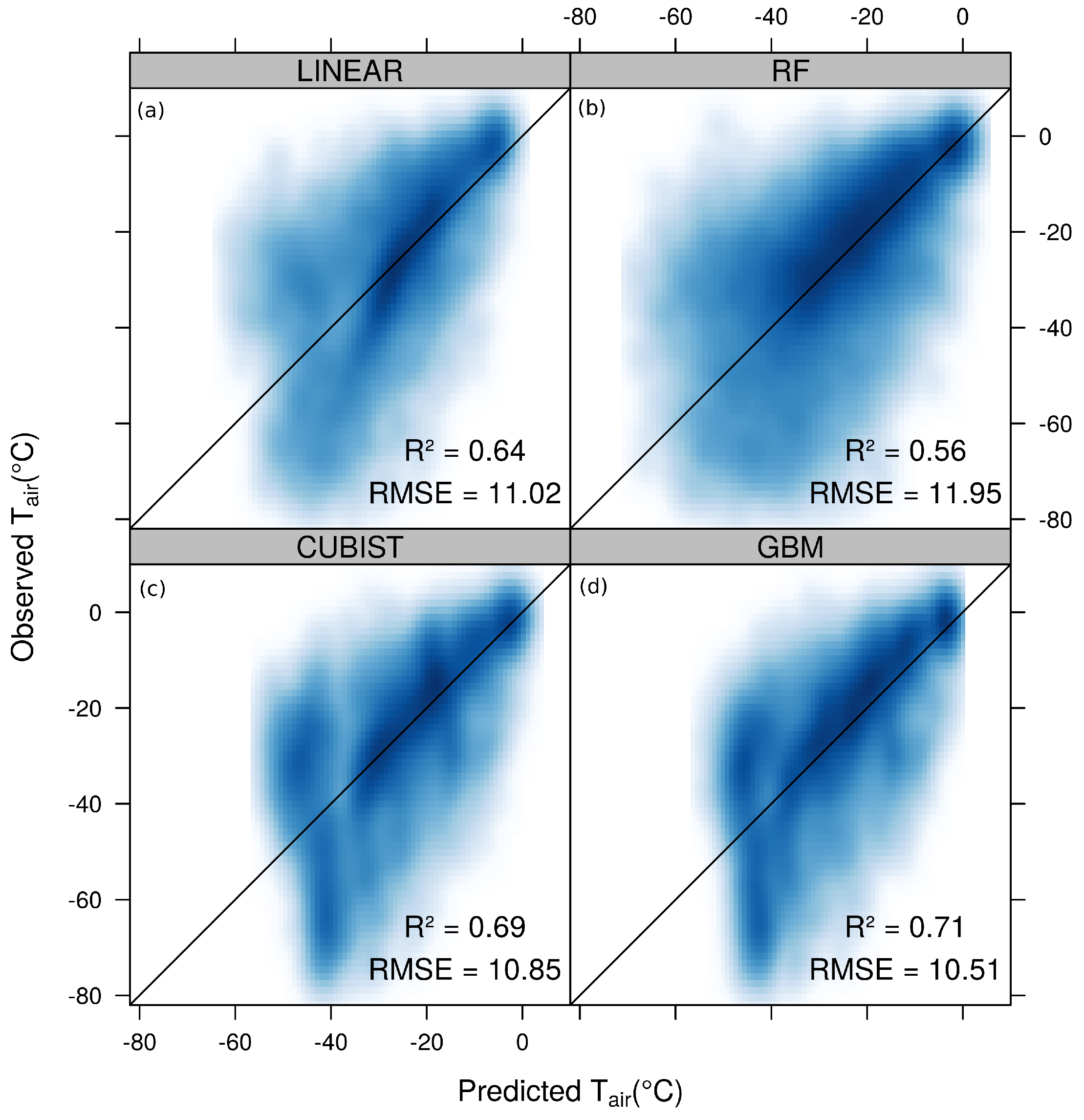
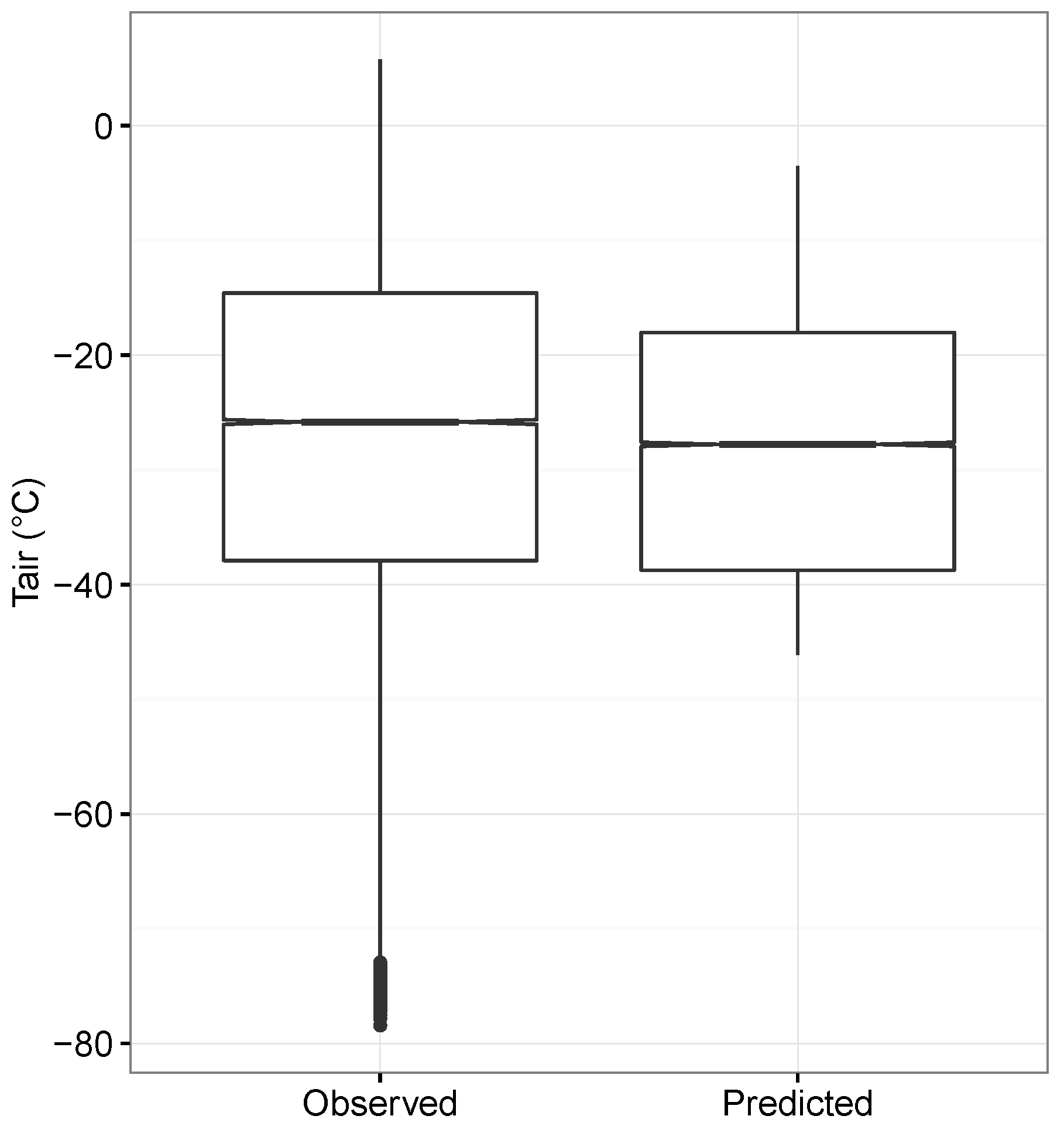
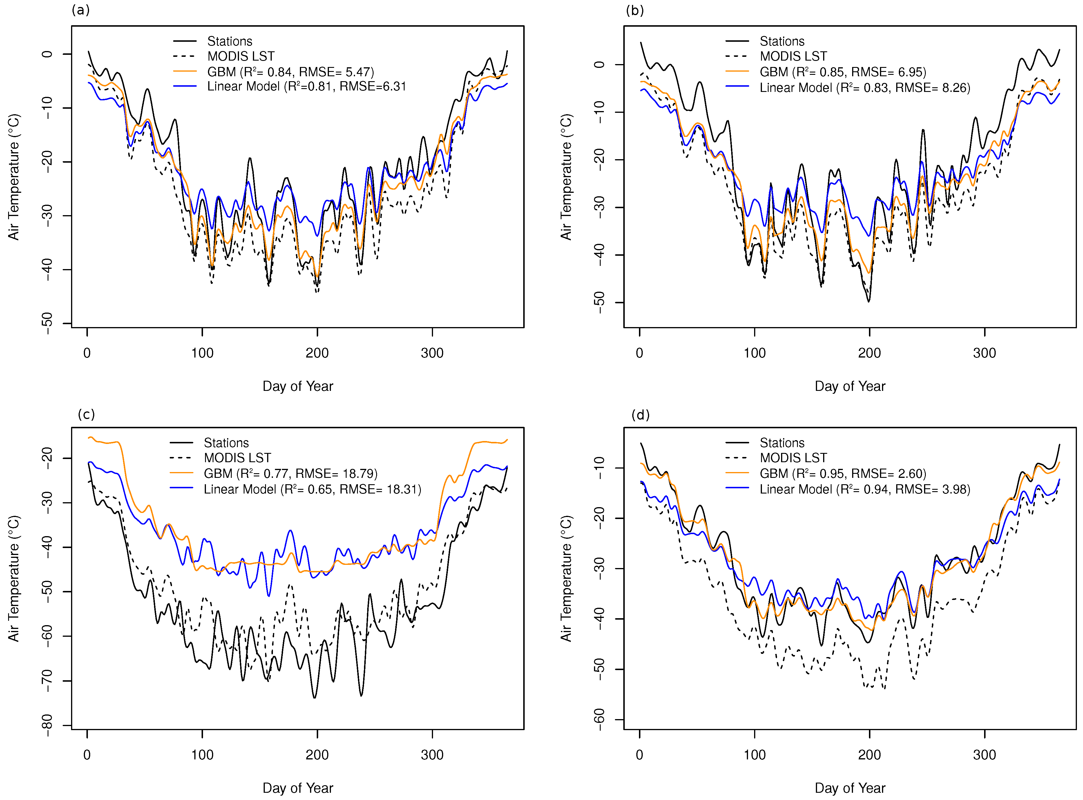
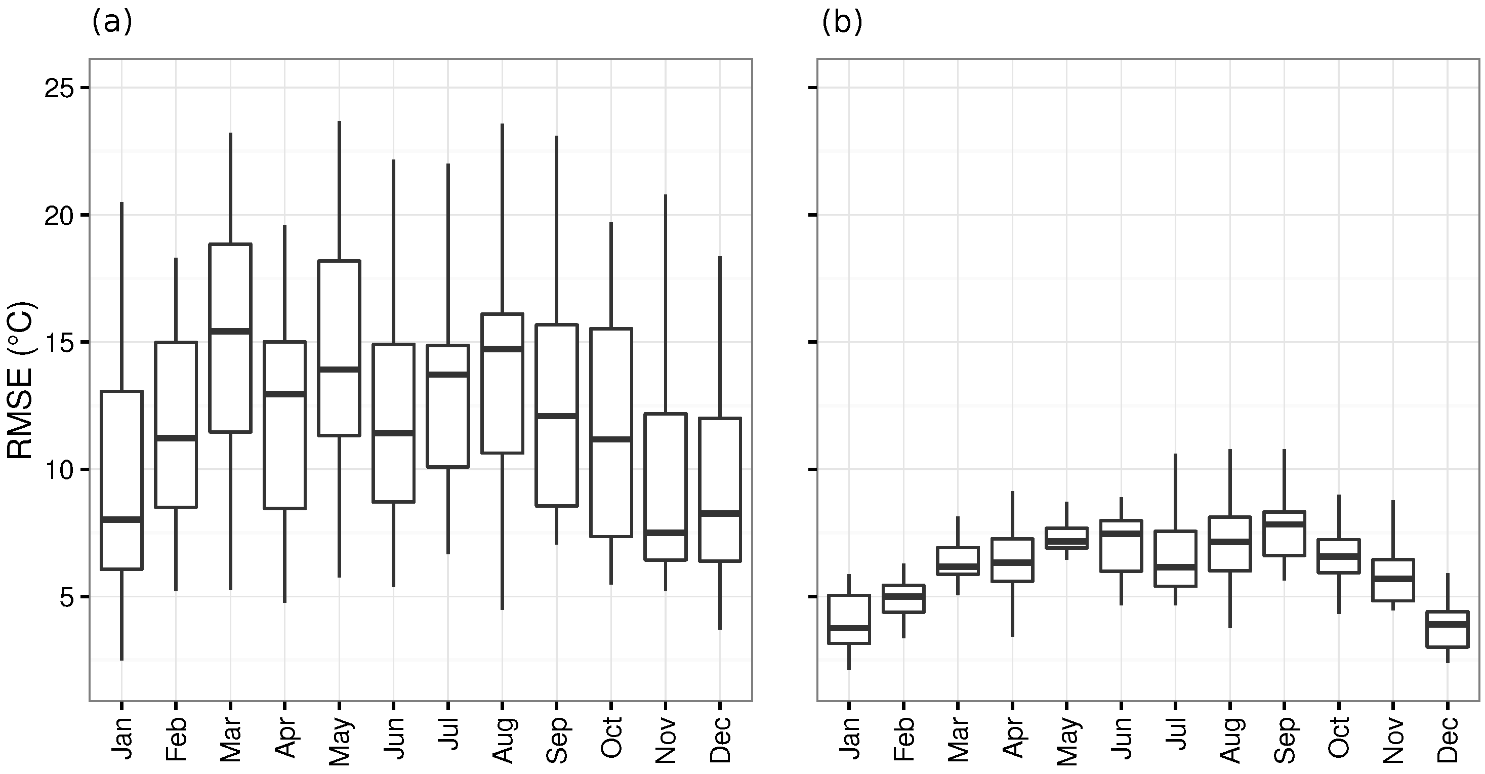
3.2. Model Comparison and Evaluation

The linear model has the form $T_{air}$ = 0.66× LST − 3.99. The model was able to predict $T_{air}$ with a LOSOCV $R^2$ of 0.64 and a RMSE of 11.02 ${}^{\circ }$C. GBM was identified as the best performing algorithm (Figure 4) with a $R^2$ of 0.71 and a RMSE of 10.51 ${}^{\circ }$C. The tuned and trained GBM model was therefore chosen as the final model to create the $T_{air}$ product. Cubist performed slightly worse than GBM (RMSE = 10.85 ${}^{\circ }$C, $R^2$ = 0.69) and the differences to the linear model were small. RF showed the lowest performance among the tested algorithms (RMSE = 11.95 ${}^{\circ }$C, $R^2$ = 0.56).

In the following, we focus on the GBM model, since this model was applied in the creation of the final $T_{air}$ product. In order to further assess characteristics of the model predictions, the model was applied to the full dataset.

The interquartile ranges of the measured and predicted data were similar (Figure 5). However, the model was not able to predict very high or very low values. Since low $T_{air}$ values (<40 ${}^{\circ }$C) were still frequently measured by the weather stations, the main weakness of the model was the inability to predict low temperatures.

Figure 6 shows a comparison between the measured and predicted time series of example weather stations (Figure 6a–c), as well as of the average time series of all 32 weather stations (Figure 6d). The seasonal $T_{air}$ patterns were generally well captured both by the LST and by the predicted $T_{air}$ time series. Compared to the linear model, the GBM model could differentiate between summer and winter months and was therefore closer to the measured time series of the McMurdo Dry Valleys (Figure 6a,b), as well as of the average time series. During winter, no clear advantage of GBM over the linear model could be observed for the McMurdo Dry Valleys (Figure 6a,b). Both models fail in the prediction of the time series of “Harry” which is located on ice and has considerably lower measured temperature values (Figure 6c). Regarding the average time series, GBM outperformed the linear model during both, summer and winter.

On average, the RMSE between measured and predicted values was significantly higher in the winter months (e.g., Jul, Aug) than in the summer months (e.g., Jan, Dec) (Figure 7). This holds especially true for the weather stations that are located on ice-free areas such as the McMurdo Dry Valleys (Figure 7b). In general, the errors were significantly lower for the weather stations in ice-free areas compared to the stations located on ice (p < 0.01) (Figure 7 and Figure 8). Regarding the stations located on ice, those in the west and south had the lowest RMSE. Apart from this observation, no clear spatial patterns could be observed for these stations (Figure 8).

When the product was aggregated to daily, weekly or monthly data the agreement between measured and predicted $T_{air}$ increased with the aggregation level (p < 0.01, Figure 9). Figure 10 shows the final product aggregated to monthly data.

4. Discussion

GBM using LST and month as predictors was the best performing model. Nevertheless, the simple linear estimation of $T_{air}$ from LST is competitive in Antarctica where no considerable land cover differences occur. However, the machine learning algorithms including the month as additional predictor were better able to approximate the time series of the weather stations.

The weakness of the model was the prediction of very low temperatures (approx. below $-35$ ${}^{\circ }$C), where the accordance between measured and predicted $T_{air}$ decreased. A direct comparison of the performance of the Antarctica $T_{air}$ product to other studies is difficult, not only due to differing environments and temporal scales, but most particularly due to different validation methods being used. Benali et al., Hengl et al. and Shi et al. [15,43,44] found considerably higher agreement between measured and predicted $T_{air}$ by including auxiliary variables in their models (RMSE usually below 2.5 ${}^{\circ }$C). However, their model training and validation strategies do not rely on LOSOCV. Since LOSOCV is considered to be a stricter validation strategy [41], it is not surprising that the agreement was better in these studies. Keeping in mind that the model performance in our study was considerably higher without LOSOCV compared to the LOSOCV performance (Figure 3a,b), it is likely that using a similar validation approach would lead to less divergent results.

Forward feature selection in conjunction with LOSOCV allowed removing variables that led to overfitting. Particularly the terrain related variables caused this problem. One characteristic of these variables is that they change in space but not in time which means that each weather station has a unique combination of these variables. We assume that these “static variables” are prone to overfitting since they are overrepresented in the predictor dataset. The weather station dependent combination of unique properties is quasi-comparable to an ID of the stations which is then used as predictor variable. Using an ID as predictor, the model would be able to fit general characteristics of the individual time series which are, however, not valid for unknown locations. Therefore, these variables need to be checked using feature selection in conjunction with LOSOCV and removed if they are misleading.

Though the LOSOCV performance could be improved using selected predictor variables only, the new $T_{air}$ product is afflicted with considerable errors that need to be explained. A first explanation comes from the characteristic of machine learning algorithms which are not able to predict extreme values (i.e., very low and very high temperatures) [24]. However, since the model also showed high errors in the $T_{air}$ range that was well represented in the training data, this probably only slightly contributed to the overall error.

It could be shown that the weather stations located in ice-free areas could be predicted with much higher accuracy compared to the weather stations located on ice which could not be solved by including the information of ice as predictor variable. Though the MODIS LST product is cloud masked, we realized that cirrus clouds could not reliably be removed from the data. Due to the “white on white” and “cold on cold” problem [45,46], cloud classification over Antarctica is challenging in winter months and over snow or ice covered areas. This causes $T_{air}$ predictions in winter months and over snow and ice covered areas more prone to errors than in summer months and/or over ice-free areas. Also Janatian et al. [21] reported a significant decrease of model performance to predict $T_{air}$ in low temperatures which might also be a result of inaccurate cloud masking in cold environments.

Another issue that likely affects the model performance is that, due to the remoteness of Antarctica, the maintenance of weather stations is challenging, and the number of stations available for ground truthing is very limited. Due to the difficulty of maintenance, the data are likely afflicted with higher errors than those of less remote areas. Errors in the data used as ground truth can have a high impact on the model outcome. An extensive quality check of the weather station data would be important in future extensions of this study.

We found no systematic patterns of accuracy for the stations located on ice. This suggests that the causes for the low performance are due to local influences rather than due to systematic errors in the LST product. Very local microclimatic influences that cannot be captured by the 1km resolution are a potential explanation but also the suggested errors in the station data. Therefore, a station-specific assessment of error sources is a future task in view to an improvement of the results.

Despite the errors, the $T_{air}$ product is of high value for scientific studies in Antarctica. The advantage is the high temporal (sub-daily to daily), as well as spatial resolution which could only be achieved using remote sensing data. The estimates provide instantaneous Tair information at the time of overpass of the Terra and Aqua satellites. These instantaneous estimates are useful to feed models that require high temporal resolution $T_{air}$ estimates. However, a variety of studies might be more interested in temporal aggregates of the product, such as on weekly or monthly scales. In this context it is of note that the simple averaging to daily composites, as performed in this study, could be improved by considering the diurnal $T_{air}$ cycle [47].

The product allows to monitor the spatio-temporal dynamics of $T_{air}$, not only on a continental scale, but also in a regional scale for example for the McMurdo Dry Valleys. The $T_{air}$ product can be considered as a baseline dataset to understand the regional and local climate variability of Antarctica. This especially applies to research areas requiring a spatially coherent gridded dataset for regional climate model evaluation in terms of linking local meteorological processes, such as topographically induced warming and cooling events, to non-local atmospheric circulation patterns (such as low pressure systems). However, it is of note that the product is currently not suitable to analyse patterns of small temperature changes. As an example, the estimated increase of $T_{air}$ by 2.4 ± 1.2 ${}^{\circ }$C over the West Antarctic Ice Sheet since the 1950s [45] will most likely not be captured. Against the background of the relevance of climate change, an improvement of the product will be required. However, a variety of ecological studies focus on the ice-free areas of Antarctica and on the summer months where organisms are active [48]. In this context, the product provides $T_{air}$ estimates with acceptable errors, especially when temporal aggregates (weekly, monthly) are considered.

The model was trained using data from 2013 only. To extend the model over the entire MODIS lifespan (MODIS LST is available since 2000), it will be necessary to include a subset of data from further years for model training to ensure that a wider range of inter-annual environmental conditions is included. Since the month was revealed as the second important predictor variable, it is important to include data from further years into training to avoid an overfitting to this specific year. At this point, the advantage of the linear model is of note which has shown a comparable performance. Since this model relied on LST solely, and we presume that the relation between LST and $T_{air}$ is not strongly affected between interannual changes (except for sensor degradation), it can directly be applied beyond the training year 2013.

It is of note that the relationship between LST and Tair is influenced by various other parameters that could not be employed in this study. Mean wind speed and direction could be responsible for horizontal heat advection, while near-surface wind turbulence allows for surface-atmosphere energy exchange through the sensible and latent heat flux. In further studies, it might be worth to combine the LST data with regional climate model results that estimate parameters such as the surface energy balance components (net surface radiation, sensible, latent and ground heat flux).

5. Conclusions

A methodology was presented to predict $T_{air}$ from MODIS LST and auxiliary data using machine learning algorithms. LST and month of the year were the most suitable and robust predictors for $T_{air}$. Among the tested models, GBM was the most promising algorithm. However, the differences to the commonly used simple linear approach were rather small. The main weakness of the model was failing to predict extremely low temperatures (e.g., below $-35$ ${}^{\circ }$C). The $T_{air}$ estimates are in 1km spatial and daily temporal resolution for the entire continent for the year 2013. The product is available from the authors on request. Future research needs to focus on on minimizing errors followed by an extension of the product to the overall lifespan of the MODIS sensor.

References

1. Schneider, D.P.; Reusch, D.B. Antarctic and southern ocean surface temperatures in CMIP5 Models in the context of the surface energy budget. J. Clim. 2016, 29, 1689–1716. [Google Scholar] [CrossRef]
2. Appelhans, T.; Mwangomo, E.; Hardy, D.R.; Hemp, A.; Nauss, T. Evaluating machine learning approaches for the interpolation of monthly air temperature at Mt. Kilimanjaro, Tanzania. Spat. Stat. 2015, 14A, 91–113. [Google Scholar] [CrossRef]
3. Hofstra, N.; Haylock, M.; New, M.; Jones, P.; Frei, C. Comparison of six methods for the interpolation of daily, European climate data. J. Geophys. Res.-Atmos. 2008, 113, D21110. [Google Scholar] [CrossRef]
4. Jarvis, C.H.; Stuart, N. A Comparison among strategies for interpolating maximum and minimum daily air temperatures. Part II: The interaction between number of guiding variables and the type of interpolation method. J. Appl. Meteor. 2001, 40, 1075–1084. [Google Scholar] [CrossRef]
5. Stahl, K.; Moore, R.; Floyer, J.; Asplin, M.; McKendry, I. Comparison of approaches for spatial interpolation of daily air temperature in a large region with complex topography and highly variable station density. Agric. For. Meteorol. 2006, 139, 224–236. [Google Scholar] [CrossRef]
6. Lazzara, M.A.; Weidner, G.A.; Keller, L.M.; Thom, J.E.; Cassano, J.J. Antarctic automatic weather station program: 30 years of polar observation. Bull. Amer. Meteor. Soc. 2012, 93, 1519–1537. [Google Scholar] [CrossRef]
7. Wang, Y.; Hou, S. A new interpolation method for Antarctic surface temperature. Prog. Nat. Sci. 2009, 19, 1843–1849. [Google Scholar] [CrossRef]
8. Rhee, J.; Im, J. Estimating high spatial resolution air temperature for regions with limited in situ data using MODIS products. Remote Sens. 2014, 6, 7360–7378. [Google Scholar] [CrossRef]
9. Gallo, K.; Hale, R.; Tarpley, D.; Yu, Y. Evaluation of the relationship between air and land surface temperature under clear- and cloudy-sky conditions. J. Appl. Meteor. Climatol. 2011, 50, 767–775. [Google Scholar] [CrossRef]
10. Vancutsem, C.; Ceccato, P.; Dinku, T.; Connor, S.J. Evaluation of MODIS land surface temperature data to estimate air temperature in different ecosystems over Africa. Remote Sens. Environ. 2010, 114, 449–465. [Google Scholar] [CrossRef]
11. Colombi, A.; De Michele, C.; Pepe, M.; Rampini, A. Estimation of daily mean air temperature from MODIS LST in alpine areas. EARSeL eProced. 2007, 6, 38–46. [Google Scholar]
12. Zhu, W.; Lü, A.; Jia, S. Estimation of daily maximum and minimum air temperature using MODIS land surface temperature products. Remote Sens. Environ. 2013, 130, 62–73. [Google Scholar] [CrossRef]
13. Sohrabinia, M.; Zawar-Reza, P.; Rack, W. Spatio-temporal analysis of the relationship between LST from MODIS and air temperature in New Zealand. Theor. Appl. Climatol. 2014, 119, 567–583. [Google Scholar] [CrossRef]
14. Mostovoy, G.V.; King, R.L.; Reddy, K.R.; Kakani, V.G.; Filippova, M.G. Statistical estimation of daily maximum and minimum air temperatures from MODIS LST data over the state of Mississippi. GISci. Remote Sens. 2006, 43, 78–110. [Google Scholar] [CrossRef]
15. Benali, A.; Carvalho, A.; Nunes, J.; Carvalhais, N.; Santos, A. Estimating air surface temperature in Portugal using MODIS LST data. Remote Sens. Environ. 2012, 124, 108–121. [Google Scholar] [CrossRef]
16. Neteler, M. Estimating daily land surface temperatures in mountainous environments by reconstructed MODIS LST Data. Remote Sens. 2010, 2, 333–351. [Google Scholar] [CrossRef]
17. Huang, R.; Zhang, C.; Huang, J.; Zhu, D.; Wang, L.; Liu, J. Mapping of daily mean air temperature in agricultural regions using daytime and nighttime land surface temperatures derived from TERRA and AQUA MODIS data. Remote Sens. 2015, 7, 8728–8756. [Google Scholar] [CrossRef]
18. Kilibarda, M.; Hengl, T.; Heuvelink, G.B.M.; Gräler, B.; Pebesma, E.; Perčec Tadić, M.; Bajat, B. Spatio-temporal interpolation of daily temperatures for global land areas at 1 km resolution. J. Geophys. Res.-Atmos. 2014, 119, 2294–2313. [Google Scholar] [CrossRef]
19. Wang, Y.; Wang, M.; Zhao, J. A comparison of MODIS LST retrievals with in situ observations from AWS over the lambert glacier basin, East Antarctica. Int. J. Geosci. 2013, 4, 611–617. [Google Scholar] [CrossRef]
20. Xu, Y.; Qin, Z.; Shen, Y. Study on the estimation of near-surface air temperature from MODIS data by statistical methods. Int. J. Remote Sens. 2012, 33, 7629–7643. [Google Scholar] [CrossRef]
21. Janatian, N.; Sadeghi, M.; Sanaeinejad, S.H.; Bakhshian, E.; Farid, A.; Hasheminia, S.M.; Ghazanfari, S. A statistical framework for estimating air temperature using MODIS land surface temperature data. Int. J. Climatol. 2016. [Google Scholar] [CrossRef]
22. Emamifar, S.; Rahimikhoob, A.; Noroozi, A.A. Daily mean air temperature estimation from MODIS land surface temperature products based on M5 model tree. Int. J. Climatol. 2013, 33, 3174–3181. [Google Scholar] [CrossRef]
23. Xu, Y.; Knudby, A.; Ho, H.C. Estimating daily maximum air temperature from MODIS in British Columbia, Canada. Int. J. Remote Sens. 2014, 35, 8108–8121. [Google Scholar] [CrossRef]
24. Kuhn, M.; Johnson, K. Applied Predictive Modeling, 1st ed.; Springer: New York, NY, USA, 2013. [Google Scholar]
25. James, G.; Witten, D.; Hastie, T.; Tibshirani, R. An Introduction to Statistical Learning: With Applications in R, 1st ed.; Springer: New York, NY, USA, 2013. [Google Scholar]
26. Wan, Z. New refinements and validation of the MODIS Land-Surface Temperature/Emissivity products. Remote Sens. Environ. 2008, 112, 59–74. [Google Scholar] [CrossRef]
27. Land Processes Distributed Active Archive Center (LP DAAC). MODIS Level 3 Land Surface Temperature and Emissivity; Version 3; Land Processes DAAC: Sioux Falls, SD, USA, 2013.
28. Ackerman, S.A.; Strabala, K.I.; Menzel, W.P.; Frey, R.A.; Moeller, C.C.; Gumley, L.E. Discriminating clear sky from clouds with MODIS. J. Geophys. Res.-Atmos. 1998, 103, 32141–32157. [Google Scholar] [CrossRef]
29. Westermann, S.; Langer, M.; Boike, J. Systematic bias of average winter-time land surface temperatures inferred from MODIS at a site on Svalbard, Norway. Remote Sens. Environ. 2012, 118, 162–167. [Google Scholar] [CrossRef] [Green Version]
30. Doran, P.T.; Dana, G.; Hastings, J.T.; Wharton, R.A. McMurdo Dry Valleys Long-Term Ecological Research (LTER): LTER automatic weather network (LAWN). Antarc. J. US 1995, 30, 276–280. [Google Scholar]
31. Seybold, C.A.; Harms, D.S.; Balks, M.; Aislabie, J.; Paetzold, R.F.; Kimble, J.; Sletten, R. Soil climate monitoring projectin the ross island region of Antarctica. Soil Surv. Horiz. 2009, 50, 52–57. [Google Scholar] [CrossRef]
32. US Geological Survey. Landsat Image Mosaic of Antarctica (LIMA): U.S Geological Survey Fact Sheet 2007–3116; US Geological Survey: Reston, VA, USA, 2007.
33. Liu, H.; Jezek, K.C.; Li, B.; Zhao, Z. Radarsat Antarctic Mapping Project Digital Elevation Model; Version 2; National Snow and Ice Data Center: Boulder, CO, USA, 2015. [Google Scholar]
34. Conrad, O.; Bechtel, B.; Bock, M.; Dietrich, H.; Fischer, E.; Gerlitz, L.; Wehberg, J.; Wichmann, V.; Böhner, J. System for Automated Geoscientific Analyses (SAGA) v. 2.1.4. Geosci. Model Dev. 2015, 8, 1991–2007. [Google Scholar] [CrossRef]
35. Fretwell, P.; Pritchard, H.D.; Vaughan, D.G.; Bamber, J.L.; Barrand, N.E.; Bell, R.; Bianchi, C.; Bingham, R.G.; Blankenship, D.D.; Casassa, G.; et al. Bedmap2: Improved ice bed, surface and thickness datasets for Antarctica. The Cryosphere 2013, 7, 375–393. [Google Scholar] [CrossRef] [Green Version]
36. Kuhn, M. Caret: Classification and Regression Training, R package version 6.0-29; CRAN: Wien, Austria, 2014.
37. Ridgeway, G. gbm: Generalized Boosted Regression Models, R package version 2.1.1; CRAN: Wien, Austria, 2015.
38. Liaw, A.; Wiener, M. Classification and Regression by randomForest. R News 2002, 2, 18–22. [Google Scholar]
39. Kuhn, M.; Weston, S.; Keefer, C.; Coulter, N.; Quinlan, R. Cubist: Rule- and Instance-Based Regression Modeling, R package version 0.0.18; CRAN: Wien, Austria, 2014.
40. Revolution Analytics.; Weston, S. doParallel: Foreach Parallel Adaptor for the Parallel Package, R package version 1.0.8; CRAN: Wien, Austria, 2014.
41. Gasch, C.K.; Hengl, T.; Gräler, B.; Meyer, H.; Magney, T.S.; Brown, D.J. Spatio-temporal interpolation of soil water, temperature, and electrical conductivity in 3D + T: The Cook Agronomy Farm data set. Spat. Stat. 2015, 14A, 70–90. [Google Scholar] [CrossRef]
42. Guyon, I.; Elisseeff, A. An introduction to variable and feature selection. J. Mach. Learn. Res. 2003, 3, 1157–1182. [Google Scholar]
43. Hengl, T.; Heuvelink, G.B.M.; Perčec Tadić, M.; Pebesma, E.J. Spatio-temporal prediction of daily temperatures using time-series of MODIS LST images. Theor. Appl. Climatol. 2011, 107, 265–277. [Google Scholar] [CrossRef]
44. Shi, L.; Liu, P.; Kloog, I.; Lee, M.; Kosheleva, A.; Schwartz, J. Estimating daily air temperature across the Southeastern United States using high-resolution satellite data: A statistical modeling study. Environ. Res. 2016, 146, 51–58. [Google Scholar] [CrossRef] [PubMed]
45. Bromwich, D.H.; Nicolas, J.P.; Monaghan, A.J.; Lazzara, M.A.; Keller, L.M.; Weidner, G.A.; Wilson, A.B. Central West Antarctica among the most rapidly warming regions on Earth. Nat. Geosci. 2013, 6, 139–145. [Google Scholar] [CrossRef]
46. Allen, R., Jr.; Durkee, P.A.; Wash, C.H. Snow/Cloud Discrimination with Multispectral Satellite Measurements. J. Appl. Meteorol. 1990, 29, 994–1004. [Google Scholar] [CrossRef]
47. Jin, M.; Dickinson, R.E. Interpolation of surface radiative temperature measured from polar orbiting satellites to a diurnal cycle: 1. Without clouds. J. Geophys. Res.-Atmos. 1999, 104, 2105–2116. [Google Scholar] [CrossRef]
48. Convey, P.; Chown, S.L.; Clarke, A.; Barnes, D.K.A.; Bokhorst, S.; Cummings, V.; Ducklow, H.W.; Frati, F.; Green, T.G.A.; Gordon, S.; et al. The spatial structure of Antarctic biodiversity. Ecol. Monogr. 2014, 84, 203–244. [Google Scholar] [CrossRef] [Green Version]
Figure 1. Map of weather stations used for model training and evaluation overlayed on a Landsat composite image [32]. The McMurdo Dry Valleys are shown in detail.
Remotesensing 08 00732 g001
Figure 2. Relative variable importance revealed by Cubist for (a) the full model and (b) the model that used variables selected during forward feature selection only. Variable importance was estimated as the percentage of times each variable was used in the model [36].
Remotesensing 08 00732 g002
Figure 3. Agreement between measured T a i r and predicted T a i r using Cubist as modeling tool. Models were first trained using the full set of predictor variables (FULL) and second using only LST and month as predictors that were revealed during forward feature selection (FFS). Two different validation strategies were used: Comparison to a 60% random subset of the total dataset (RSS), as well as Leave-One-Station-Out Cross-Validation (LOSOCV). The problem of overfitting becomes obvious by comparing the performance of the full model validated by RSS (a) with the performance of the full model validated by LOSOCV (b). Using the 2-variable model, the performance validated by RSS decreased (c) compared to the full model. Only slight differences between RSS and LOSOCV (c,d) indicate that there is no considerable overfitting in the 2-variable model. The most important point is that the 2-variable model could improve the LOSOCV performance (d) compared to the full model. Data are represented as smoothed scatter plots where the intensity of the color represent the data point density.
Remotesensing 08 00732 g003
Figure 4. Correlation between measured and predicted T a i r based on LOSOCV of (a) the linear model, (b) RF, (c) Cubist and (d) GBM. The intensity of the color represent the data point density.
Remotesensing 08 00732 g004
Figure 5. Distribution of measured T a i r compared to predicted T a i r .
Remotesensing 08 00732 g005
Figure 6. Time series of the three example weather stations (a) “Brownworth”, (b) “Bull pass” and (c) “Harry”, as well as (d) the average time series of all 32 weather stations for the year 2013. “Brownworth” and “Bull pass” are weather stations located in the McMurdo Dry Valleys. “Harry” is located on ice. The lines represent the measured T a i r (solid black), MODIS LST (dotted black), GBM model predictions (orange), as well as linear model predictions (blue).
Remotesensing 08 00732 g006
Figure 7. Monthly RMSE of T a i r predictions separately for (a) weather stations located on ice and (b) weather stations located on ice-free areas.
Remotesensing 08 00732 g007
Figure 8. Spatial distribution of RMSE of predicted T a i r for the 32 weather station. The McMurdo Dry Valleys are shown in detail. The weather stations are overlayed on a Landsat composite image [32].
Remotesensing 08 00732 g008
Figure 9. Performance of the T a i r product on different aggregation levels.
Remotesensing 08 00732 g009
Figure 10. Monthly aggregates of T a i r as predicted by the GBM model.
Remotesensing 08 00732 g010