
Ocean Wave Parameters Retrieval from Sentinel-1 SAR Imagery


1
Marine Acoustics and Remote Sensing Laboratory, Zhejiang Ocean University, Zhoushan 316000, China
2
Global Science and Technology, National Oceanic and Atmospheric Administration (NOAA)-National Environmental Satellite, Data, and Information Service (NESDIS), College Park, MD 20740, USA
3
National Marine Data and Information Service, Tianjin 300171, China
4
Jiangsu Key Laboratory of Coast Ocean Resources Development and Environment Security, Hohai University, Nanjing 210000, China
*
Author to whom correspondence should be addressed.
Remote Sens. 2016, 8(9), 707; https://doi.org/10.3390/rs8090707
Submission received: 15 April 2016
/
Revised: 5 August 2016
/
Accepted: 23 August 2016
/
Published: 27 August 2016
Abstract
:In this paper, a semi-empirical algorithm for significant wave height (Hs) and mean wave period (Tmw) retrieval from C-band VV-polarization Sentinel-1 synthetic aperture radar (SAR) imagery is presented. We develop a semi-empirical function for Hs retrieval, which describes the relation between Hs and cutoff wavelength, radar incidence angle, and wave propagation direction relative to radar look direction. Additionally, Tmw can be also calculated through Hs and cutoff wavelength by using another empirical function. We collected 106 C-band stripmap mode Sentinel-1 SAR images in VV-polarization and wave measurements from in situ buoys. There are a total of 150 matchup points. We used 93 matchups to tune the coefficients of the semi-empirical algorithm and the rest 57 matchups for validation. The comparison shows a 0.69 m root mean square error (RMSE) of Hs with a 18.6% of scatter index (SI) and 1.98 s RMSE of Tmw with a 24.8% of SI. Results indicate that the algorithm is suitable for wave parameters retrieval from Sentinel-1 SAR data.

1. Introduction
Space-borne synthetic aperture radar (SAR) has been used to detect wave information in a large coverage (10 × 10 km2 to 400 × 400 km2) with high spatial resolution (up to 1 m). At present, SAR data is available from C-band (5.3 GHz) Radarsat-2 and Sentinel-1; X-band (9.8 GHz) TerraSAR-X with its twins TanDEM-X, and Cosmo-SkyMed; and L-band (1.2 GHz) ALOS-2 satellites. Much effort has been devoted for marine applications from SAR over past decades, especially for wind and wave retrieval [1]. Wave parameters, e.g., significant wave height (Hs) and mean wave period (Tmw), are usually obtained from SAR-derived wave spectra. Traditionally, the methodology of wave spectra retrieval needs a good understanding of complicated SAR wave imaging mechanisms typically explained by the two-scale model, including the tilt and hydrodynamic modulations [2] on sea surface short waves. However, there is a specific non-linear distortion of SAR wave imaging, named velocity bunching [3], due to the relative motion of the sea surface waves to a satellite platform, that leads to waves shorter than a specific wavelength not detectable by SAR [4,5].
Traditionally, there are three types of wave retrieval algorithms from single-polarization SAR data. The first type includes theoretical-based algorithm, such as the Max-Planck Institute (MPI) [6,7], semi-parametric retrieval algorithm (SPRA) [8,9], parameterized first-guess spectrum method (PFSM) [10,11,12], and the partition rescaling and shift algorithm (PARSA) [13,14]. They all rely on the first-guess wave spectra, which can be obtained from numeric ocean wave models or be calculated from parametric functions, such as the Jonswap function [15]. The second type includes empirical algorithms, such as CWAVE_ERS [16], CWAVE_ENVI [17]. Although these second-type algorithms do not require prior wind information from either SAR-derived or other sources, they only work for ERS-2 or Envisat-ASAR wave mode data. Therefore, wave parameters inverted by using these algorithms depend on the accuracy of prior wind information. Recently, there is a new way to extract wave information from normalized radar cross section (NRCS) measured by SAR [18]. That algorithm has designed an empirical function between Hs and NRCS without using the complex hydrodynamic modulation transfer function (MTF). The coefficients of the algorithm were tuned from five HH-polarization ScanSAR mode Radarsat-1 hurricane images and the Third Generation Ocean Wave Prediction Model (WAM) operational results [19].
For fully-polarimetric synthetic aperture radar, algorithms [20,21] are usually based on the wave slope estimation between different band SAR images. Polarimetric SAR wave retrieval algorithms yield reasonable results against buoy measurements [22], and currently the only free and open SAR data source is from the available two-channel C-band Sentinel-1 SAR, either in VV- and VH-polarization or in HH- and HV-polarization.
Parallel to the satellite flight is defined as the azimuth direction, and radar look direction is the range direction. Due to the relative motion between sea surface wave and satellite platform, there is a Doppler frequency shift that exists in the azimuth direction. Doppler frequency shift induces a cutoff in the SAR spectra in the azimuth direction [23]. This mechanism is known as velocity bunching. In other words, the non-linear modulation of velocity bunching leads to sea surface waves shorter than a specific wavelength in the azimuth direction being undetectable. In particular, systematic comparison between SAR-derived azimuth cutoff wavelength and buoy measurements is established in [24] through a large amount of ENVISAT-ASAR wave mode data, showing a 12.79 m root mean square error (RMSE) of azimuth cutoff wavelength. It is well known that the cutoff wavelength is related not only to wind speed, but also significant wave height [25]. Recently, some work has been devoted for developing the Hs retrieval algorithms by using only SAR-derived cutoff wavelength [26,27]. Collectively, it was found that Hs was linearly related to the cutoff wavelength. An empirical function, which only depends on polarization, was developed from C-band Radarsat-2 data [27] and conveniently applied for Hs estimation. The Hs derived from empirical function are validated against in situ buoy measurements and the RMSE is 0.87 m. However, as mentioned in [27], the cutoff wavelength should be dependent on radar incidence angle and wave propagation direction relative to radar look direction, as well as Hs.
In this paper, we included the cutoff wavelength, radar incidence angle, and wave propagation direction to propose a semi-empirical algorithm for wave parameters retrieval. We also built an empirical function, which allows estimating Tmw by using inverted Hs and the cutoff wavelength. In the literature [27], the radar incidence angle and wave propagation direction were not included in the empirical algorithm.
We organize the paper as follows: the C-band VV-polarization Sentinel-1 SAR images and in situ buoy data are in Section 2. In Section 3, we present the methodology of deriving the empirical function for Hs retrieval. Then how to tune the coefficients by using the 93 matchup data from C-band VV-polarization Sentinel-1 SAR images is presented in Section 4. SAR wave retrieval validation against buoy measurements is discussed in Section 5. Conclusions are in Section 6.
2. Data Description
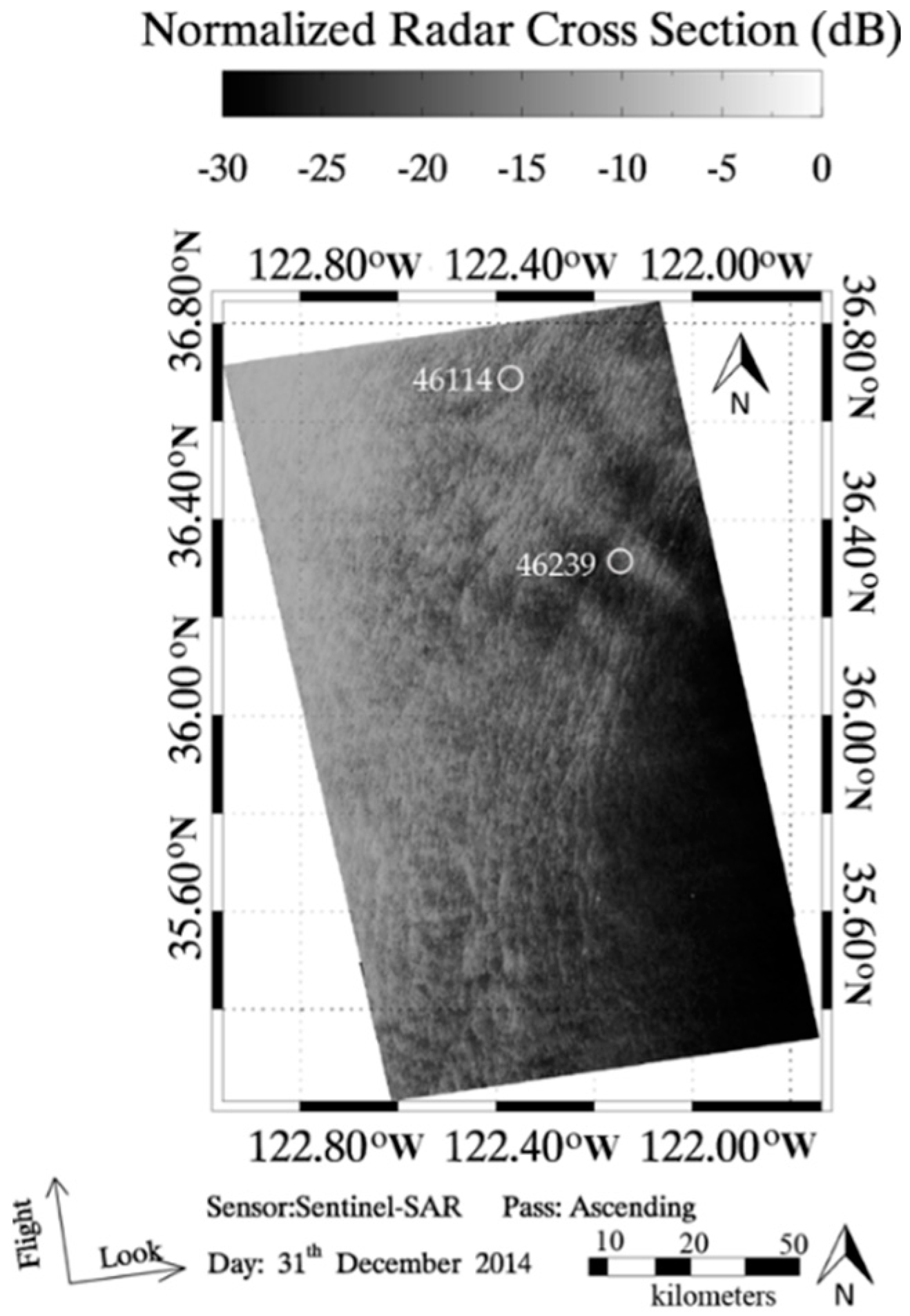
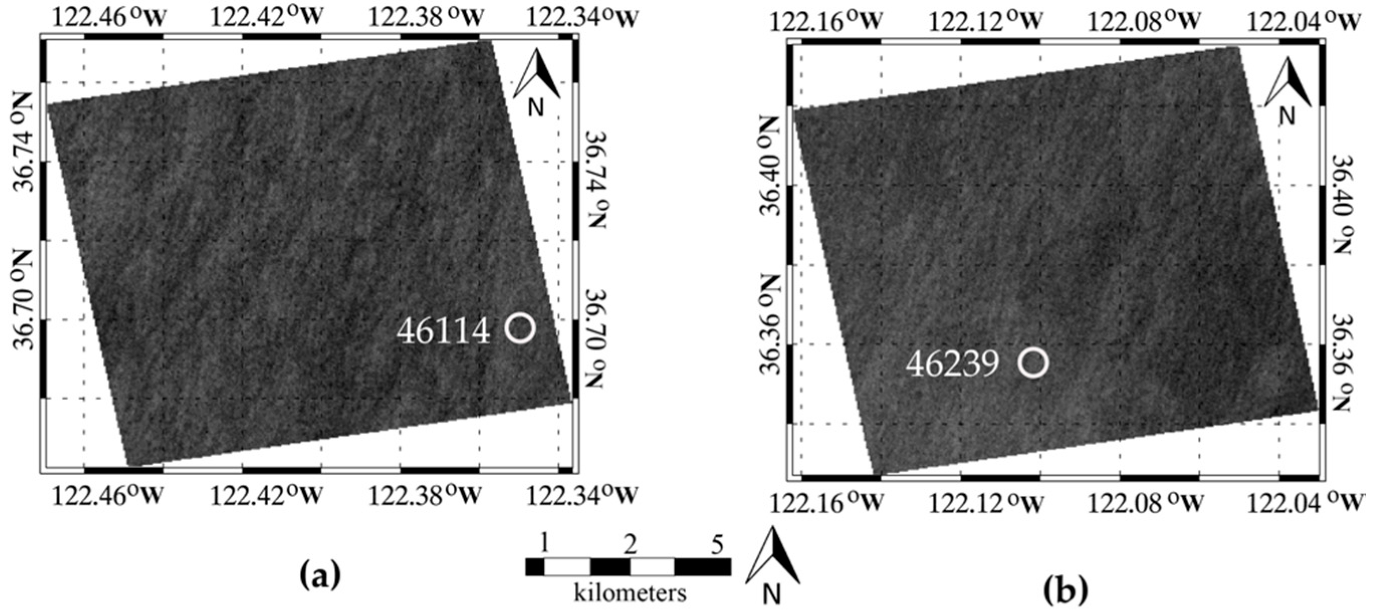
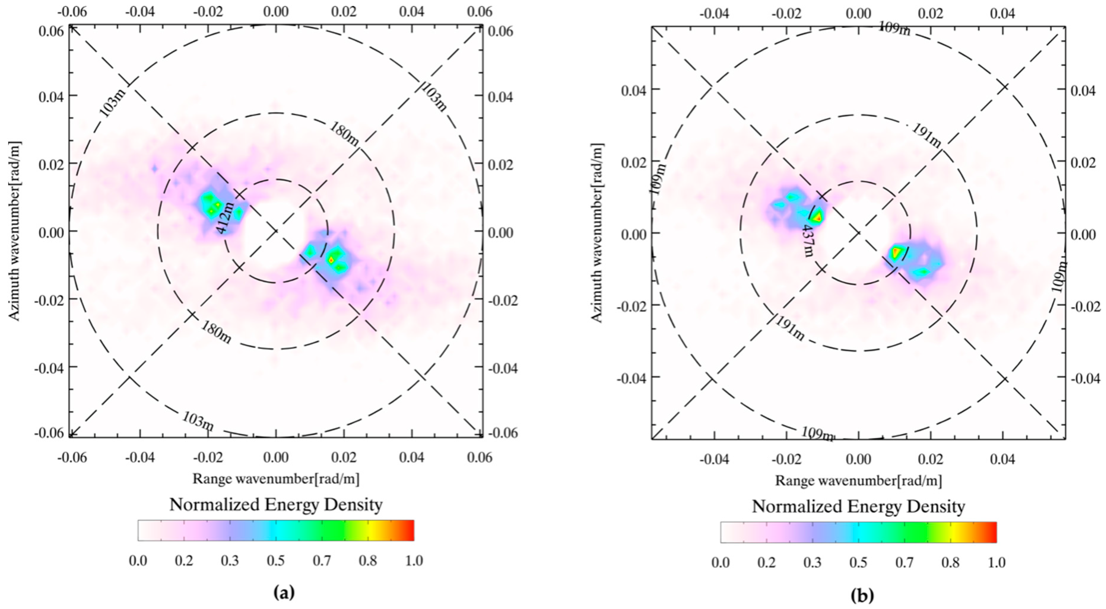
The Sentinel-1 SAR satellite was launched by European Space Agency in April 2014. It operates in C-band with different polarizations and beam modes. We collected a total of 106 stripmap mode Sentinel-1 SAR images acquired in VV-polarization in U.S. coastal waters during the period of April 2014 through January 2016 in this study. The radar incidence angle ranges from 20° to 47°. The coverage of each image contains at least one National Data Buoy Center (NDBC) buoy location. As an example, a SAR image acquired at 02:06 UTC on 31 December 2014 in Western U.S. coastal waters is shown in Figure 1. The white circles represent the locations of corresponding buoys (IDs: 46114 and 46239). Sentinel-1 SAR has a high spatial resolution ranging from 10 to 20 m in our data collection. We extracted two 1024 × 1024 pixel sub-scenes centered at the two buoy locations, which have a coverage of around 200 km2 and shown in Figure 2a,b. Although a bit of distortion by rainfall exists in the image, which may affect homogeneity of the sea surface backscattering, good-quality power spectra of NRCS of Figure 2a,b can be obtained by using the two-dimensional Fast Fourier Transform (FFT) method, as shown in Figure 3a,b.
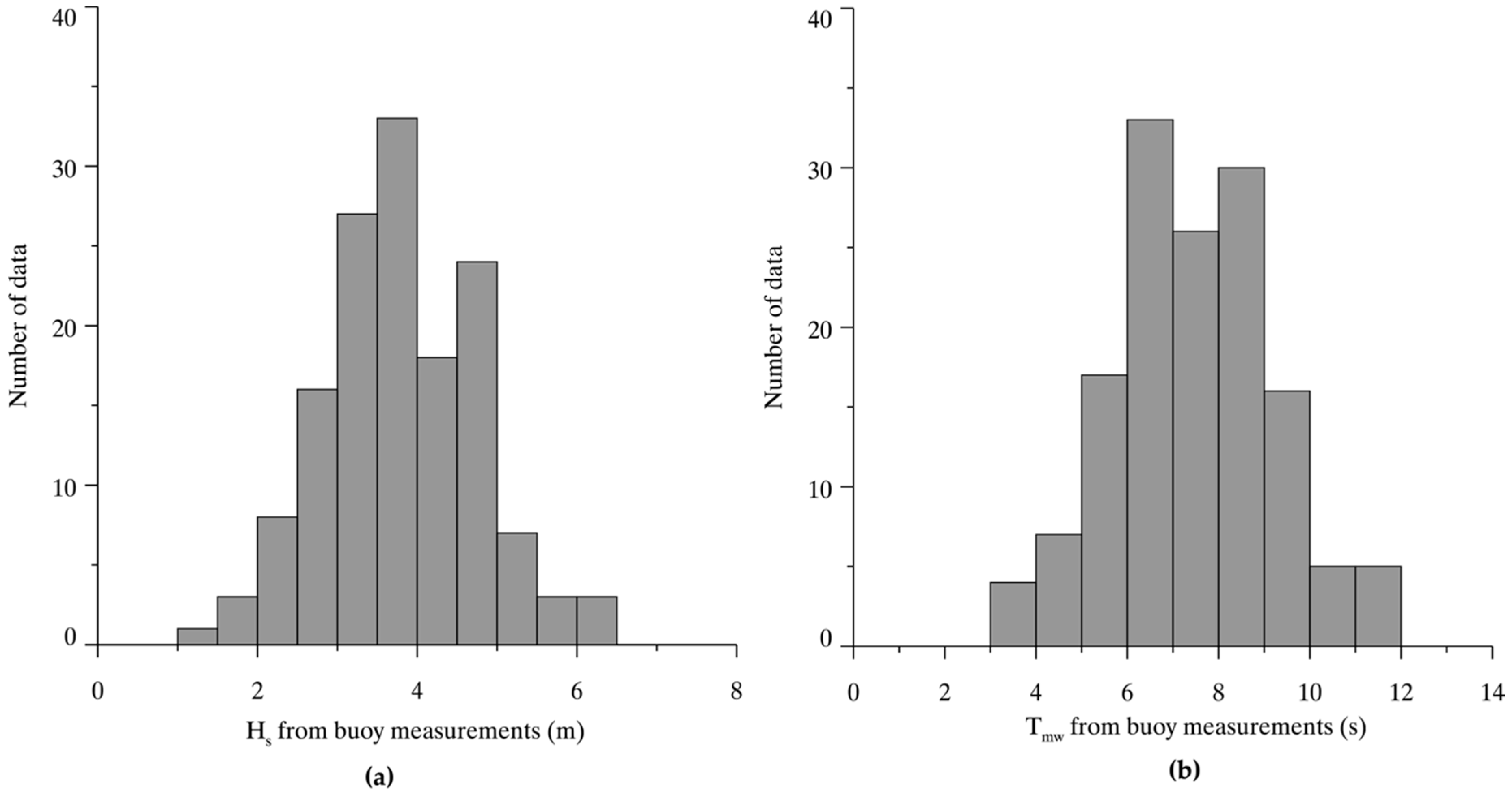
Among the 106 Sentinel-1 SAR images, we found 150 Hs and Tmw matchup data from collocated buoy measurements. In our data collection, if we obtain a good-quality power spectrum of NRCS from a Sentinel-1 sub-scene centered at a buoy location, we believe the spectra represents the actual eave spectra. Wave parameters are measured at an interval of 10 min from in situ buoy measurements. We choose the values of wave parameters from buoy measurements at the time, which are closest to SAR imaging time. Therefore, the time difference between buoys and SAR measurements is within 5 min. Ninety-three matchup points were used for tuning our algorithm, and 57 were used to validate the algorithm. We also used buoy-measured wind directions to determine the sea state to see whether wind-sea or swells dominate the study area. Histograms of collocated buoy data are shown in Figure 4, in which the Hs and Tmw range from 1 to 7 m and 3 to 12 s, respectively.
3. Methodology
3.1. A Semi-Empirical Model for Hs Retrieval
The cutoff wavelength has been theoretically derived in [6] through the modulation transfer function (MTF). Since the cutoff wavelength is related to wind speed, it is also important to get accurate wind information. Compared to wave retrieval from SAR, wind retrieval is a much more matured technology. As a matter of fact, many geophysical model functions (GMFs) have been developed to retrieve wind speed from SAR at different band and polarization with known accuracy [28,29,30,31,32,33,34].
The dependency of cutoff wavelength on significant wave height was demonstrated in [35]:
wherein λc is the cutoff wavelength, β is the satellite range-to-velocity parameter, is the velocity bunching transfer function, ω is the wave frequency, and Sω is the one-dimensional wave spectra. We have:
where, R is the slant range, V is the satellite flight velocity, θ is the radar incidence angle, ϕ is the wave propoagation direction relative to radar look direction. Hs can be calculated by Equation (4):
Substituting Equations (3) and (4) into Equation (1), the relation between Hs and λc can be written as:
Although, it is impossible to solve Equation (5) directly due to the unknown variable Sω, Hs can be determined by the factor of λc/β. Based on this thought, a simply empirical function was built in [26] by relating Hs to λc and β.
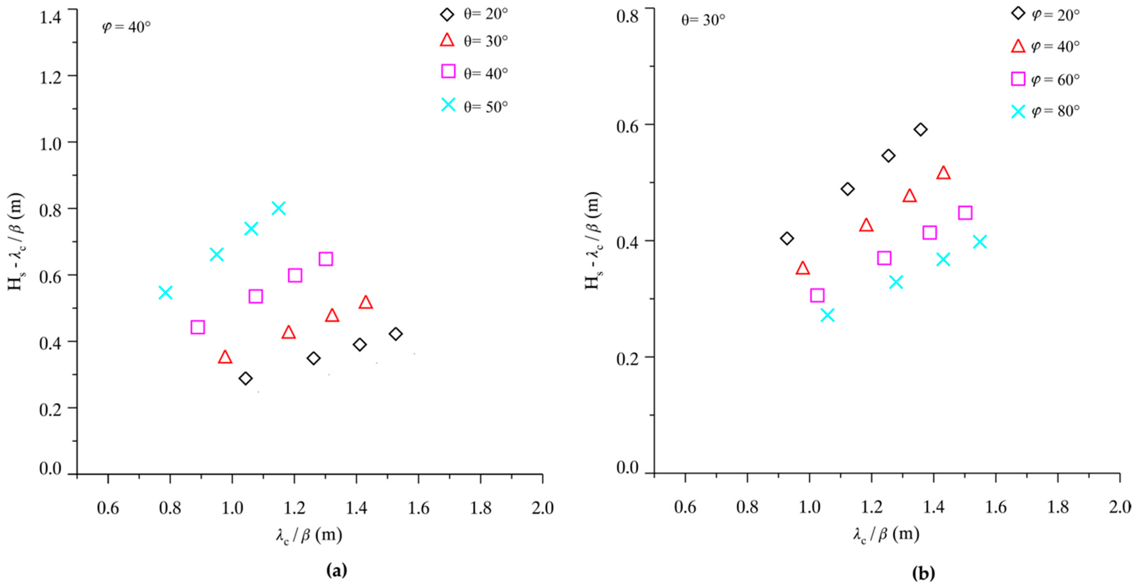
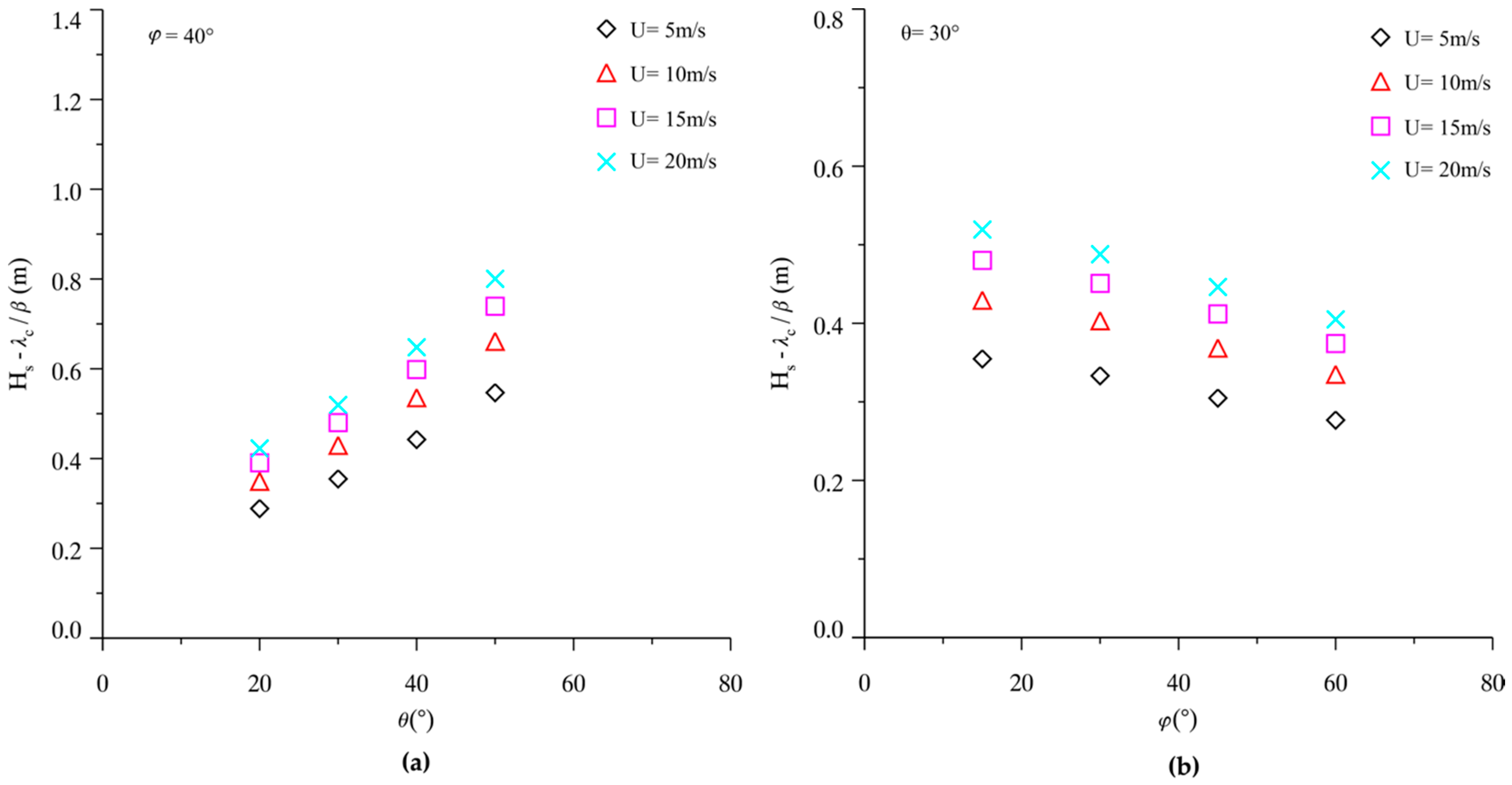
The widely used Jonwap wave spectra model is employed to simulate the Sω at the wind speed U of 5, 10, 15, and 20 m/s. Then, Hs can be obtained from Jonswap simulation and value of λc/β is calculated by Equation (5). The Hs−λc/β, that is <λc/β> versus λc/β at various θ and a fixed ϕ is shown in Figure 5a. The incidence angle θ varies from 30° to 60° at interval of 10° and wave propagation direction relative to range direction ϕ is fixed at 40°. Similarly, in Figure 5b, θ is fixed at 30° and ϕ varies from 20° to 80° at an interval of 20°. Figure 5a,b show that Hs is quasi-linearly related to the λc/β at each θ and ϕ. This relationship is also true in [27] when the author used the Wen wave spectra [36] and PM wave spectra [37]. At ϕ = 40°, the relationship between <λc/β> and θ for different U is shown in Figure 6a. It is found that <λc/β> increases when the radar incidence angle θ increases. Figure 6b shows the relation between <λc/β> and ϕ, in which θ is fixed at 30°. <λc/β> decreases when ϕ increases. This phenomenon is reasonable, because the velocity bunching is negatively related to the wave propagation angle relative to range direction ϕ and passively related to incidence angle θ. In other words, velocity bunching becomes weaker as ϕ increases and stronger as θ increases.
Following the idea proposed in [27], together with the above analysis, we can propose a more complete semi-empirical function to retrieve Hs by adding the radar incidence angle θ and wave propagation angle relative to the range direction ϕ to the original algorithm that only contained cutoff wavelength λc:
wherein the coefficient matrix A is determined from the matchup dataset using the least-square-fit method. The coefficents are shown in Table 1. The empirical function allows retrieving Hs without any prior information. Moreover, the advantage is that it is not restricted for application unlike CWAVE_ERS and CWAVE_ENVI, due to CWAVEs being originally designed for ERS-2 and ENVISAT-ASAR SAR wave mode data.
3.2. An Empirical Model for Tmw Retrieval
The relation between significant wave height and mean wave period has been proposed in [26], hereby we brifely introduce it. First, root-mean-square orbital velocity component ρ is defined as:
wherein Sω,φ is the two-dimensional wave spectra in wave frequency ω and wave direction relative to azimuth direction φ (φ = 90 − ϕ), we take Dω,φ is the normalized directional distribution function:
After submitting Equation (8) into Equation (7), we obtain:
where:
and Cω is the second cosine coefficient of Dω,φ [38], having a following relation with φ:
wherein:
and Bω is the second sine Fourier coefficient.
Thus the cutoff wavelength λc is simplified as:
and Tmw is:
from Equations (4), (12), and (13), the Tmw can be caluculated from Hs and λc:
Since the variable G is unknown in Equation (15), Tmw cannot be directly calculated. Therefore, we propose an empirical function for Tmw retrieval, which depends on the value of Hs × (β/λc):
wherein the coefficient matrix B is determined from the matchup data by using the least-square-fit method, as shown in Table 2.
One can see that both Hs and Tmw are the function of the cutoff wavelength estimation λc, radar incidence angle θ, and wave propagation relative to range direction ϕ; all can be directly obtained from the SAR data.
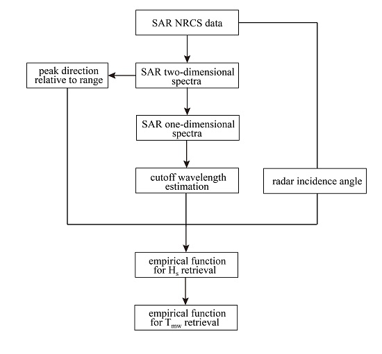
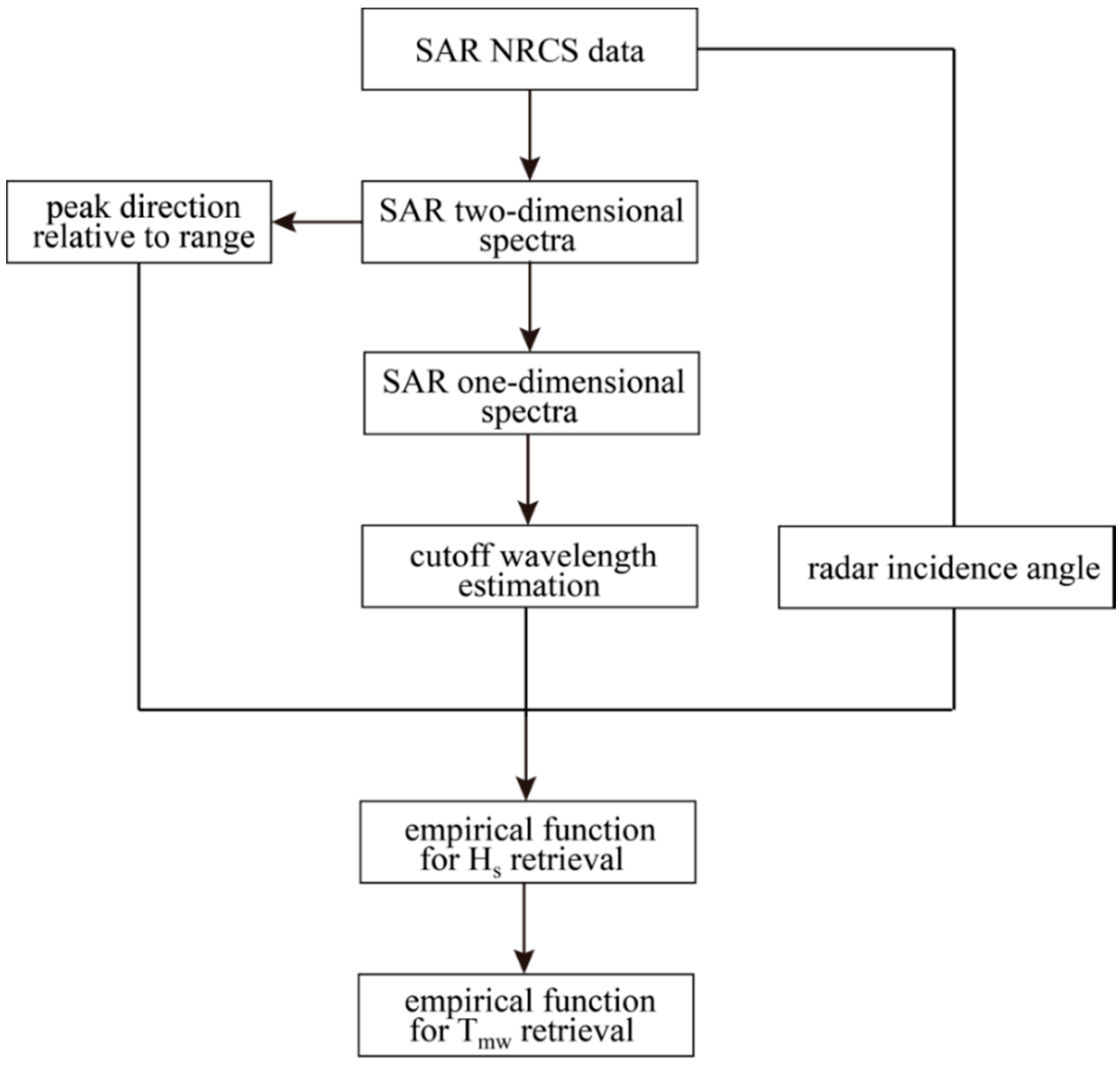
The block diagram of the scheme of semi-empirical algorithm for wave parameters retrieval based on cutoff wavelength estimation is shown in Figure 7. First, the two-dimensional SAR image spectra is calculated from NRCS by using two-dimensional FFT method. Since the SAR spectra has 180-degree ambiguity with two peaks, we use the one between 0° and 90°, instead of finding the true wave propagation direction. One can see below that selecting one peak does not affect the final calculation result. Secondly, one-dimensional SAR spectra is obtained by integrating the two-dimensional SAR spectra in the range direction in order to estimate the cutoff wavelength. And then Hs is calculated from SAR-derived cutoff wavelength λc, radar incidence angle θ and peak wave direction relative to range direction ϕ by using Equation (6). Finally, Tmw is calculated by using Equation (16).
4. Tuning the Algorithm
A total of 93 sub-scenes centered at buoy locations in stripmap mode C-band VV-polarization Sentinel-1 SAR images are extracted. As for each sub-scene, we need to calculate each cutoff wavelength λc estimation, radar incidence angle θ, and wave peak direction relative to range direction ϕ.
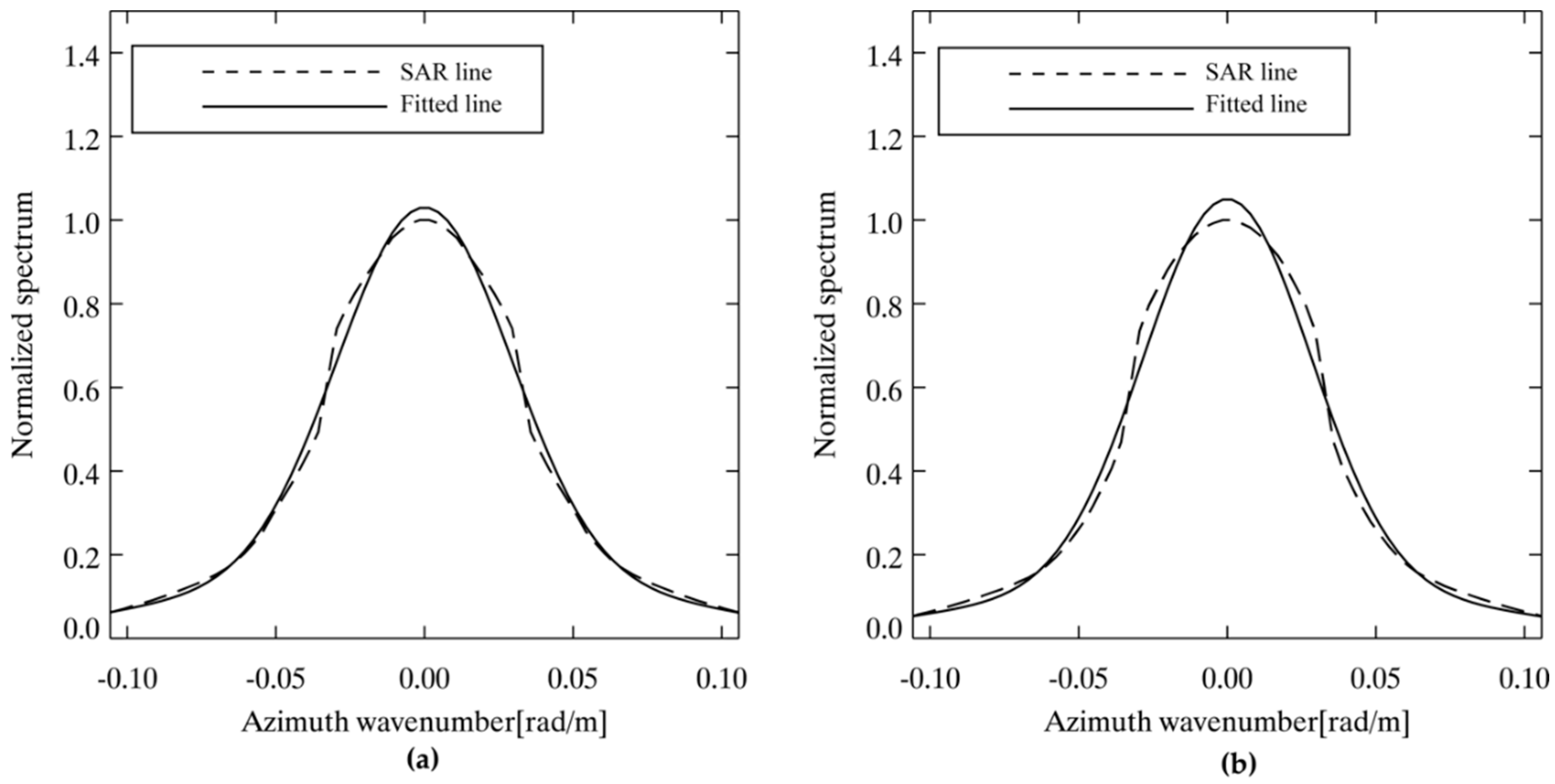
An example below is used to illustrate the processing chain. The C-band VV-polarization Sentinel-1 SAR image taken at 02:06 UTC on 31 December 2014 was analyzed. The Sentinel-1 SAR spectra of sub-scene of Figure 2a,b is shown in Figure 3a,b, respectively. Then the two-dimensional SAR spectra with Gaussian fit function is integrated in the range direction. The Gaussian fit function has the formulation as exp{π(kx/kc)}, in which kx is the wavenumber in the azimuth direction and kc = 2π/λc is the cutoff wavenumber. The Gaussian fitted results are illustrated in Figure 8a,b corresponding to Figure 3a,b.
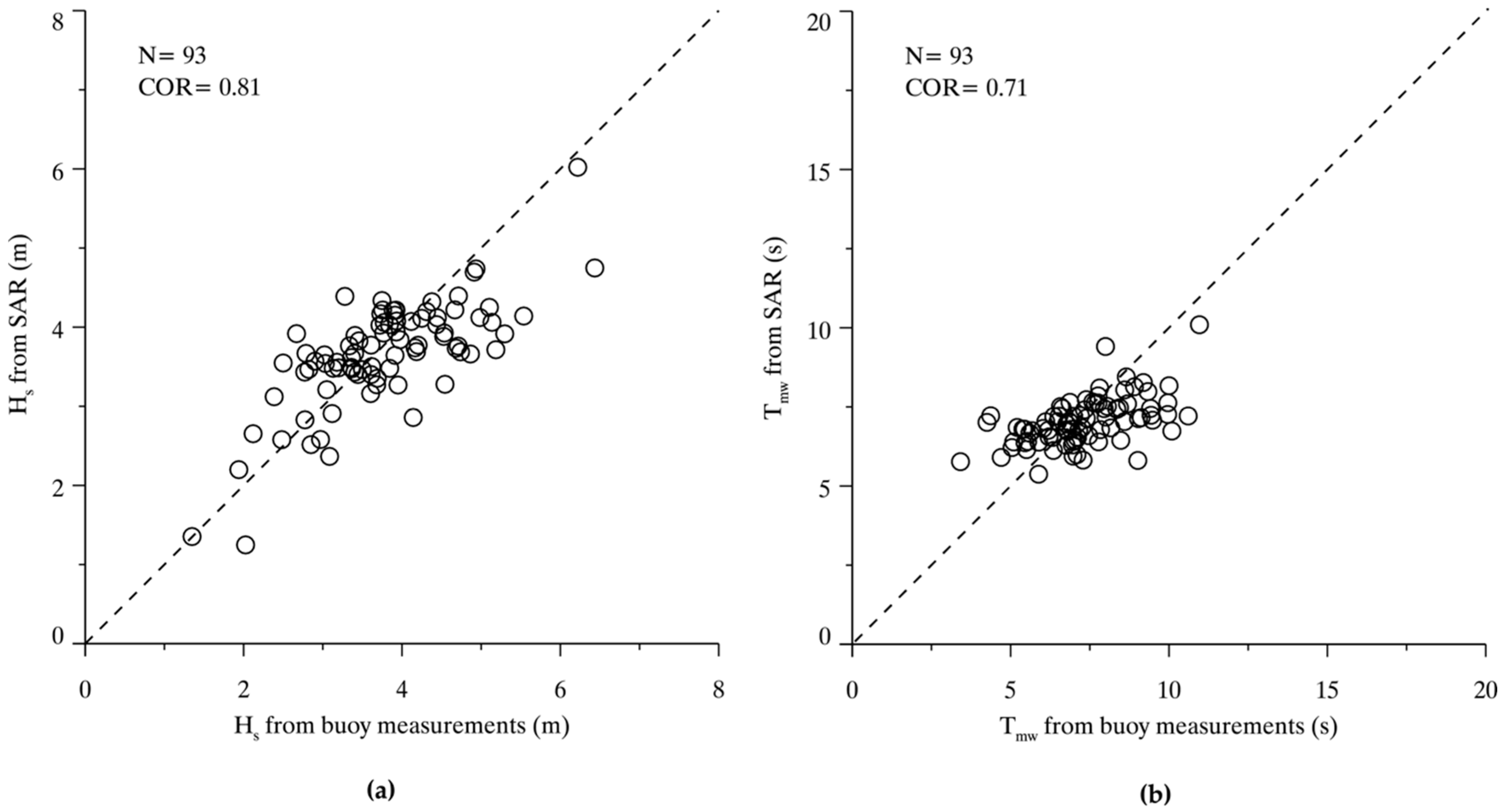
We then matchup these analysis results, including the cutoff wavelength λc, radar incidence angle θ, and wave peak direction relative to range direction ϕ, with Hs and Tmw measurements from in situ buoys. The coefficients in Equations (6) and (16) are then derived. The values of matrix A in Equation (6) and B in Equation (16) are shown in Table 1 and Table 2, respectively. The correlation (COR) between the fitted results and buoy measurements for 93 matchup points is 0.81 and 0.71 for Hs and Tmw respectively, as shown in Figure 9. Under this circumstance, we think the semi-empirical algorithm is suitable for wave retrieval and we will discuss the validation of our algorithm in the next section.
5. Discussions
Out of the 93 matchup data for tuning our algorithm, the remaining 57 matchup data points are used for validation. Buoy wind directions are used to distinguish the wind sea from swell-dominant cases. We compare the peak directions with wind directions.
Wind direction is measured from in situ buoys. For example, the wind direction is assumed to range from 0° to 90°, clockwise relative to north, and that wind blows from northeast to southwest. Then, the two peak directions with a 180° ambiguity from two-dimensional SAR spectra is obtained by meteorological convention. If the peak direction from two-dimensional SAR spectra ranges from 90° to 180° or 270° to 360°, clockwise relative to north, we think that is a swell-dominant case due to the wave propagation direction being in conflict with the wind direction. Oppositely, if the peak direction from two-dimensional SAR spectra ranges from 0° to 90° or 180° to 270°, we think that is wind-sea dominant case. Thus, we separate the validation into two categories: wind sea and swell.
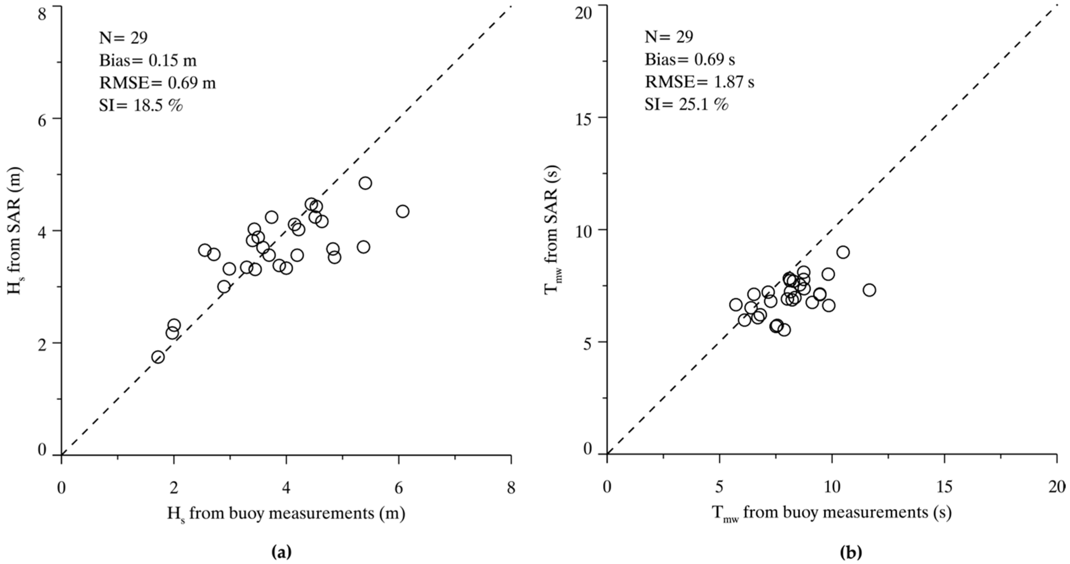
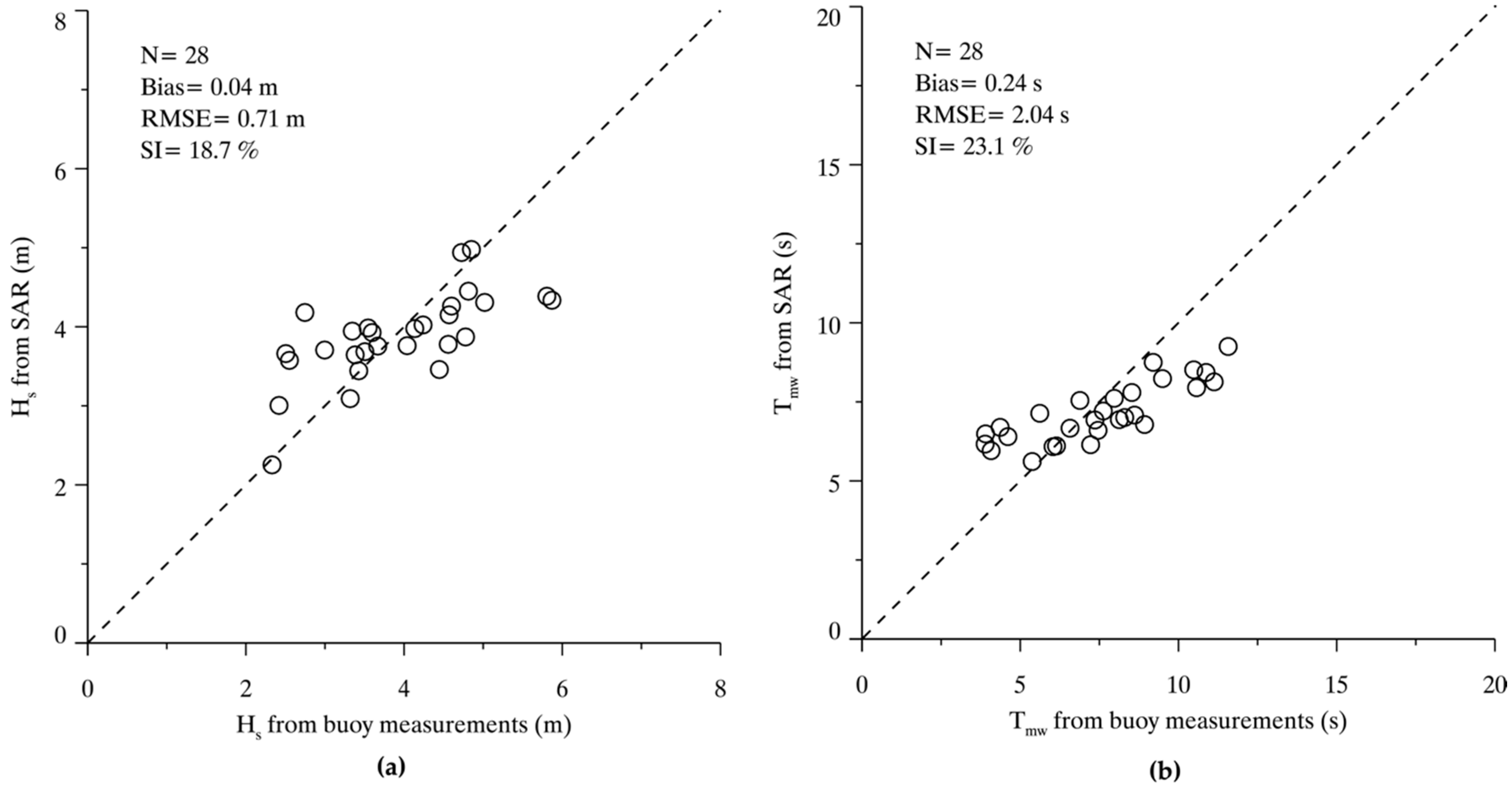
The Hs from Equation (6) and Tmw from Equation (14) for 29 wind-sea dominant cases were compared to buoy measurements in Figure 10a,b, respectively. It is shown that the RMSE of Hs is 0.69 m with an SI of 18.5% and RMSE of Tmw is 1.87 s with a 25.1% of SI. Similarly, RMSE of Hs is 0.71 m with an 18.7% of SI and RMSE of Tmw is 2.04 s with a 23.1% of SI for 28 swell-dominant cases (Figure 11a,b). Although it is found that the semi-empirical algorithm works for both wind-sea and swell sea state, the algorithm performs slightly better for wind-sea dominant cases than swell dominant cases studied from our data collection.
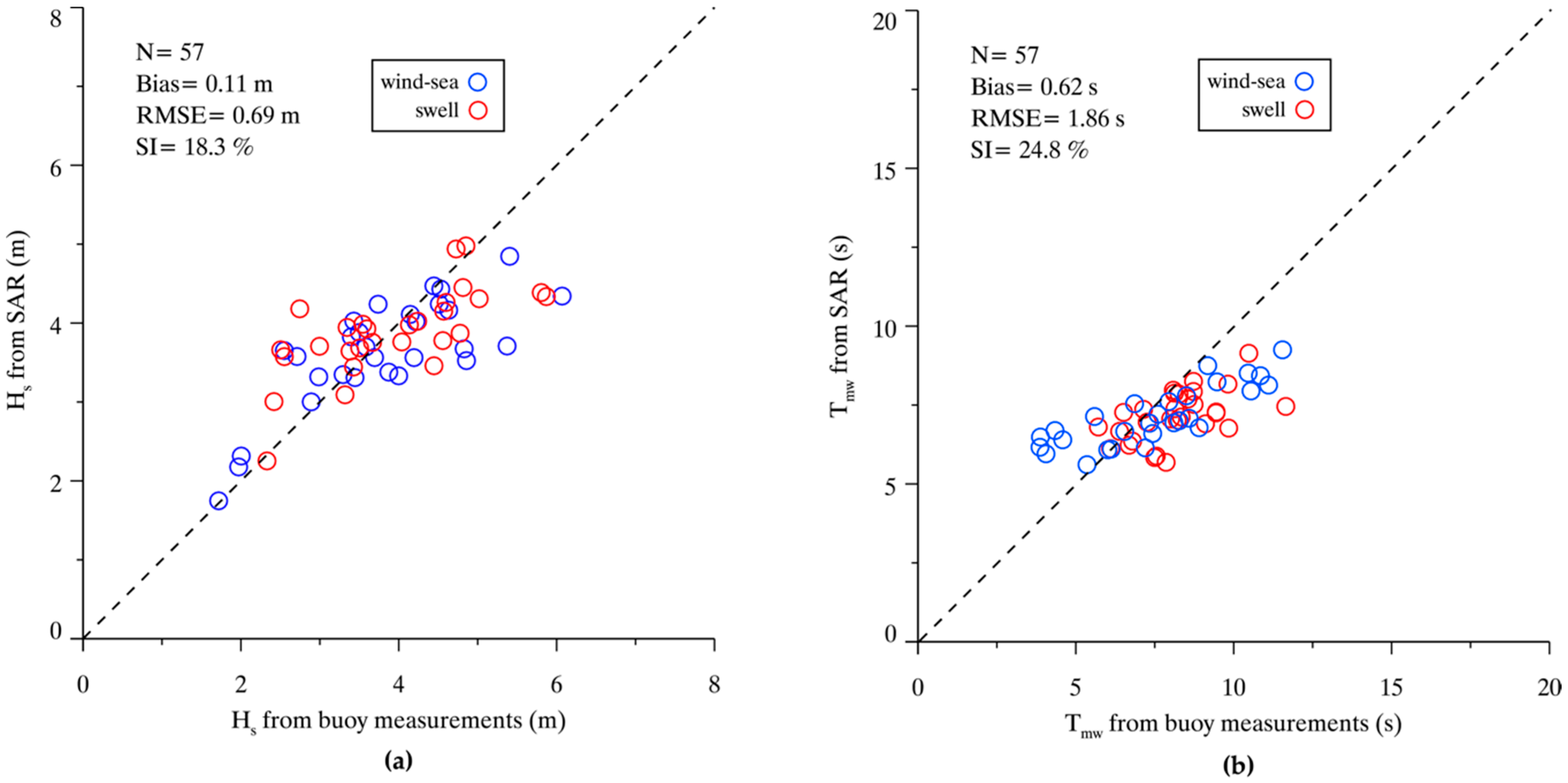
We show the validation of a total of 57 cases in Figure 12, showing the RMSE of Hs is 0.69 m with an SI of 18.3% and RMSE of Tmw is 1.86 s with a 24.8% of SI. Referring to the achievements of several studies for wave retrieval from C-band SAR data, the standard deviation (SDE) of Hs ranges from 0.4 to 0.7 m against in situ buoy measurements or numeric wave model results [8,12,13,14,21]. The semi-empirical algorithm herein is expected to work well for various types of C-band SAR data. It is more applicable than existed CWAVE models, because CWAVEs were specifically tuned to derive wave information from ERS-2 and ENVISAT-ASAR wave mode data. The CWAVE model cannot be directly used for wave retrieval from SAR image mode data. In addition, statistical results (an RMSE of 0.69 m of Hs) of our semi-empirical algorithm outperformed the traditional empirical function proposed in [27] (an RMSE of 0.87 m of Hs).
6. Conclusions
At present, all algorithms for wave retrieval from C-band single polarization SAR, e.g., VV- or HH-polarization, depend on prior information, e.g., first-guess wave spectra or wind speed. In this paper, we propose a semi-empirical algorithm for wave parameters retrieval from C-band Sentinel-1 images in VV-polarization. Firstly, the empirical function for Hs retrieval is basically designed from the simulation between Hs−λc/β and λc/β, which is similar to the linear function in [27]. In particular, the dependency of radar incidence angle and wave propagation direction is also included in our empirical function. Then, the similar empirical function, which is designed from the relation between significant wave height and mean wave period proposed in [26], is used to calculate Tmw.
A total of 106 Sentinel-1 VV-polarization images together with measurements from in situ buoys were collected to develop and to validate the algorithm. The coefficients in the functions for Hs and Tmw retrieval are determined from 93 collocated data, including the SAR-derived cutoff wavelength λc, radar incidence angle θ, peak direction relative to range at two-dimensional SAR spectra ϕ, and the measurements from in situ buoys. Although the semi-empirical algorithm was tuned from 93 matchup data, the correlation between fitted results and measurements from in situ buoys is 0.81 for Hs and 0.71 for Tmw. We think the proposed algorithm can be applied for wave retrieval.
Fifty-seen matchup points are used to validate the algorithm. The validation results show a 0.69 m RMSE of Hs with a 18.3% of SI and 1.86 s RMSE of Tmw with a 24.8% of SI. Based on the wind directions from in situ buoy measurements and the direction of dominant wave spectra, we separate the ocean into wind sea and swell regimes and validate the algorithm separately. There are 29 wind-sea dominant cases and 28 swell dominant cases. Comparisons show that RMSE of Hs is 0.69 m with a 18.5% of SI and RMSE of Tmw is 1.87 s with a 25.1% of SI for 29 wind-sea cases. It is also shown that RMSE of Hs is 0.71 m with a 18.7% of SI and RMSE of Tmw is 2.04 s with a 23.1% of SI for 28 swell dominant cases. Known from other achievements, the SI of Hs by using the existing wave retrieval algorithms against other sources are around 20%. The comparisons indicate that the accuracy of retrieval results by using our semi-empirical algorithm is acceptable in this study.
Empirical models, CWAVE_ERS and CWAVE_ENVI, can be employed to estimate Hs and Tmw from ERS-2 and ENVISAT-ASAR wave mode data only. Our algorithm provides a conveniently empirical method to retrieve Hs and Tmw from C-band VV-polarization Sentinel-1 SAR images, including, but not limited to, stripmap mode data. However, we plan to further implement the algorithm in hurricane and typhoon conditions, in order to confirm the validation of the semi-empirical algorithm under extreme sea states.
In summary, the proposed semi-empirical algorithm is applicable for wave parameters from various band and different polarization SAR data, such as X-band and L-band. Therefore, it is expected that the wind and waves can be simultaneously measured from single-polarization SAR data.
Acknowledgments
The C-band Sentinel-1 SAR images are provided by European Space Agency via https://scihub.copernicus.eu. Buoy data are downloaded via http://www.ndbc.noaa.gov/. The research is partly supported by the Zhejiang Provincial Natural Science Foundation of China under Grant No. LQ14D060001, Public Welfare Technical Applied Research Project of Zhejiang Province under Grant No. 2015C31021, Jiangsu Key Laboratory of Coast Ocean Resources Development and Environment Security under Grant JSCE201505 and Scientific Foundation of Zhejiang Ocean University (2015). The views, opinions, and findings contained in this report are those of the authors and should not be construed as an official NOAA or U.S. Government position, policy or decision.
Author Contributions
Weizeng Shao and Xiaofeng Li came up the original idea and designed the experiments; Weizeng Shao and Zheng Zhang analyzed the data; Huan Li and Zheng Zhang collected the data; all authors contributed to the writing and revising of the manuscript.
Conflicts of Interest
The authors declare no conflict of interest.
References
- Chapron, B.; Johnsen, H.; Garello, R. Wave and wind retrieval from SAR images of the ocean. Ann. Telecommun. 2001, 56, 682–699. [Google Scholar]
- Valenzuela, G.R. Theories for the interaction of electromagnetic and oceanic waves—A review. Bound-Lay Meteorol. 1978, 13, 61–85. [Google Scholar] [CrossRef]
- Alpers, W.; Ross, D.B.; Rufenach, C.L. On the detectability of ocean surface waves by real and synthetic radar. J. Geophys. Res. 1981, 86, 10529–10546. [Google Scholar] [CrossRef]
- Alpers, W.; Bruning, C. On the relative importance of motion-related contributions to SAR imaging mechanism of ocean surface waves. IEEE Trans. Geosci. Remote Sens. 1986, 24, 873–885. [Google Scholar] [CrossRef]
- Li, X.F.; Pichel, W.; He, M.X.; Wu, S.; Friedman, K.; Clemente-Colon, P.; Zhao, C. Observation of hurricane-generated ocean swell refraction at the Gulf Stream North Wall with the RADARSAT-1 synthetic aperture radar. IEEE Trans. Geosci. Remote Sens. 2002, 40, 2131–2142. [Google Scholar]
- Hasselmann, K.; Hasselmann, S. On the nonlinear mapping of an ocean wave spectrum into a synthetic aperture radar image spectrum. J. Geophys. Res. 1991, 96, 10713–10729. [Google Scholar] [CrossRef]
- Hasselmann, S.; Bruning, C.; Hasselmann, K. An improved algorithm for the retrieval of ocean wave spectra from synthetic aperture radar image spectra. J. Geophys. Res. 1996, 101, 6615–6629. [Google Scholar] [CrossRef]
- Mastenbroek, C.; de Valk, C.F. A semi-parametric algorithm to retrieve ocean wave spectra from synthetic aperture radar. J. Geophys. Res. 2000, 105, 3497–3516. [Google Scholar] [CrossRef]
- Zhang, B.; Li, X.F.; Perrie, W.; He, Y.J. Synergistic measurements of ocean winds and waves from SAR. J. Geophys. Res. 2015, 120, 6164–6184. [Google Scholar] [CrossRef]
- Sun, J.; Guan, C.L. Parameterized first-guess spectrum method for retrieving directional spectrum of swell-dominated waves and huge waves from SAR images. Chin. J. Oceanol. Limn. 2006, 24, 12–20. [Google Scholar]
- Sun, J.; Kawamura, H. Retrieval of surface wave parameters from SAR images and their validation in the coastal seas around Japan. J. Oceanogr. 2009, 65, 567–577. [Google Scholar] [CrossRef]
- Shao, W.Z.; Li, X.F.; Sun, J. Ocean wave parameters retrieval from TerraSAR-X images validated against buoy measurements and model results. Remote Sens. 2015, 7, 12815–12828. [Google Scholar] [CrossRef]
- Schulz-Stellenfleth, J.; Lehner, S.; Hoja, D. A parametric scheme for the retrieval of two-dimensional ocean wave spectra from synthetic aperture radar look cross spectra. J. Geophys. Res. 2005, 110, 297–314. [Google Scholar] [CrossRef]
- Li, X.M.; Konig, T.; Schulz-Stellenfleth, J.; Lehner, S. Validation and intercomparison of ocean wave spectra inversion schemes using ASAR wave mode data. Int. J. Remote Sens. 2010, 31, 4969–4993. [Google Scholar] [CrossRef]
- Hasselmann, K.; Barnett, T.P.; Bouws, E.; Carlson, H.; Cartwright, D.E.; Enke, K.; Ewing, J.A.; Gienapp, H.; Hasselmann, D.E.; Kruseman, P.; et al. Measurements of Wind-Wave Growth and Swell Decay During the Joint North Sea Wave Project (JONSWAP); Deutches Hydrographisches Institut: Hamburg, Germany, 1973. [Google Scholar]
- Schulz-Stellenfleth, J.; Konig, T.; Lehner, S. An empirical approach for the retrieval of integral ocean wave parameters from synthetic aperture radar data. J. Geophys. Res. 2007, 112, 1–14. [Google Scholar] [CrossRef]
- Li, X.M.; Lehner, S.; Bruns, T. Ocean wave integral parameter measurements using Envisat ASAR wave mode data. IEEE Trans. Geosci. Remote Sens. 2011, 49, 155–174. [Google Scholar] [CrossRef]
- Romeiser, R.; Graber, H.C.; Caruso, M.J.; Jensen, R.E.; Walker, D.T.; Cox, A.T. A new approach to ocean wave parameter estimates from C-band ScanSAR images. IEEE Trans. Geosci. Remote Sens. 2015, 53, 1320–1345. [Google Scholar] [CrossRef]
- The Wamdi Group. The WAM model—A third generation ocean wave prediction model. J. Phys. Oceanogr. 1988, 18, 1775–1810. [Google Scholar]
- Schuler, D.L.; Lee, J.S.; Kasilingam, D.; Pottier, E. Measurement of ocean surface slopes and wave spectra using polarimetric SAR image data. Remote Sens. Environ. 2004, 91, 198–211. [Google Scholar] [CrossRef]
- He, Y.J.; Shen, H.; Perrie, W. Remote sensing of ocean waves by polarimetric SAR. J. Atmos. Oceanic Techno. 2006, 23, 1768. [Google Scholar] [CrossRef]
- Zhang, B.; Perrie, W.; He, Y.J. Validation of RADARSAT-2 fully polarimetric SAR measurements of ocean surface waves. J. Geophys. Res. 2010, 115, 302–315. [Google Scholar] [CrossRef]
- Kerbaol, V.; Chapron, B.; Vachon, P.W. Analysis of ERS-1/2 synthetic aperture radar wave mode imagettes. J. Geophys. Res. 1998, 115, 7833–7846. [Google Scholar] [CrossRef]
- Stopa, J.E.; Ardhuin, F.; Collard, F.; Chapron, B. Estimating wave orbital velocities through the azimuth cut-off from space borne satellites. J. Geophys. Res. 2015, 120, 7616–7634. [Google Scholar] [CrossRef]
- Vachon, P.W.; Krogstad, H.E.; Paterson, J.S. Airborne and spaceborne synthetic aperture radar observations of ocean waves. Atmos. Ocean 1994, 32, 83–112. [Google Scholar] [CrossRef]
- Wang, H.; Zhu, J.; Yang, J.S. A semi-empirical algorithm for SAR wave height retrieval and its validation using Envisat ASAR wave mode data. Acta Oceanol. Sin. 2012, 31, 59–66. [Google Scholar]
- Ren, L.; Yang, J.S.; Zheng, G.; Wang, J. Significant wave height estimation using azimuth cutoff of C-band RADARSAT-2 single-polarization SAR images. Acta Oceanol. Sin. 2015, 12, 1–9. [Google Scholar] [CrossRef]
- Takeyama, Y.; Ohsawa, T.; Kozai, K.; Hasager, C.B.; Badger, M. Comparison of geophysical model functions for SAR wind speed retrieval in Japanese coastal waters. Remote Sens. 2013, 5, 1956–1973. [Google Scholar] [CrossRef] [Green Version]
- Yang, X.F.; Li, X.F.; Zheng, Q.A.; Gu, X.F.; Pichel, W.G.; Li, Z. Comparison of ocean-surface winds retrieved from Quikscat scatterometer and Radarsat-1 SAR in offshore waters of the U.S. west coast. IEEE Geosci. Remote Sens. 2011, 8, 163–167. [Google Scholar] [CrossRef]
- Hersbach, H. Comparison of C-Band scatterometer CMOD5.N equivalent neutral winds with ECMWF. J. Atmos. Ocean Tech. 2010, 27, 721–736. [Google Scholar] [CrossRef]
- Yang, X.F.; Li, X.F.; Pichel, W.G.; Li, Z. Comparison of ocean surface winds from Envisat ASAR, Metop Ascat scatterometer, buoy measurements, and NOGAPS model. IEEE Trans. Geosci. Remote Sens. 2011, 49, 4743–4750. [Google Scholar] [CrossRef]
- Shao, W.Z.; Sun, J.; Guan, C.L.; Sun, Z.F. A method for sea surface wind field retrieval from SAR image mode data. J. Ocean Univ. China 2014, 13, 198–204. [Google Scholar] [CrossRef]
- Stoffelen, A.; Anderson, D. Scatterometer data interpretation: derivation of the transfer function, CMOD4. J. Geophys. Res. 1997, 102, 5767–5780. [Google Scholar] [CrossRef]
- Hersbach, H.; Stoffelen, A.; Haan, S.D. An improved C-band scatterometer ocean geophysical model function: CMOD5. J. Geophys. Res. 2007, 112, C03006. [Google Scholar] [CrossRef]
- Marghany, M.; Ibrahim, Z.; Genderen, J.V. Azimuth cut-off model for significant wave height investigation along coastal water of Kuala Terengganu, Malaysia. Int. J. Appl. Earth Obs. 2002, 4, 147–160. [Google Scholar] [CrossRef]
- Wen, S.C.; Guo, P.F.; Zhang, D.C.; Guan, C.L.; Zhan, H.G. Analytically derived wind-wave directional spectrum part 2. characteristics, comparison and verification of spectrum. J. Oceanogr. 1993, 49, 149–172. [Google Scholar] [CrossRef]
- Pierson, W.J.; Moskowitz, L. A proposed spectral form for fully developed wind seas based on the similarity theory of S. A. Kitaigorodskii. J. Geophys. Res. 1964, 69, 5181–5190. [Google Scholar] [CrossRef]
- Longuet-Higinns, M.S.; Cartwright, D.E.; Smith, N.D. Observations of the directional spectrum of sea waves using the motions of a floating buoy. In Proceedings of the a conference on Ocean Wave Spectra, Easton, Maryland, 1–4 May 1963; pp. 111–136.
Figure 1.
An example of collected C-band VV-polarization Sentinel SAR image taken at 02:06 UTC on 31 December 2014 in the Western U.S. coastal area. The observations from buoys were measured at 02:10 UTC.
Figure 1.
An example of collected C-band VV-polarization Sentinel SAR image taken at 02:06 UTC on 31 December 2014 in the Western U.S. coastal area. The observations from buoys were measured at 02:10 UTC.

Figure 2.
The quick-look image of sub-scene, which covers the location of the buoys (a) ID: 46114; and (b) ID: 46239.
Figure 2.
The quick-look image of sub-scene, which covers the location of the buoys (a) ID: 46114; and (b) ID: 46239.

Figure 3.
Two-dimensional SAR spectra by using FFT method (a) corresponding to sub-scene of Figure 2a; and (b) corresponding to sub-scene of Figure 2b.

Figure 4.
Histograms of buoy data (a) Hs ranges from 1 to 7 m; and (b) Tmw ranges from 3 to 12 s.

Figure 5.
<λc/β> that is defined as the bias between Hs from Jonswap simulation and value of λc/β calculated by Equation (5), versus λc/β. (a) Wave propagation direction relative to the range direction ϕ is fixed at 40° and the radar incidence angle θ varies from 30° to 60° at an interval of 10°; and (b) θ is fixed at 30° and ϕ varies from 20° to 80° at an interval of 20° clockwise.

Figure 6.
(a) <λc/β> versus θ at various U from 5 to 20 m/s at an interval of 5 m/s, and ϕ is fixed at 40°; and (b) <λc/β> versus ϕ at various U from 5 to 20 m/s at an interval of 5 m/s, and θ is fixed at 30°.
Figure 6.
(a) <λc/β> versus θ at various U from 5 to 20 m/s at an interval of 5 m/s, and ϕ is fixed at 40°; and (b) <λc/β> versus ϕ at various U from 5 to 20 m/s at an interval of 5 m/s, and θ is fixed at 30°.

Figure 7.
Block diagram of the scheme of semi-empirical wave parameters retrieval, including Hs and Tmw.
Figure 7.
Block diagram of the scheme of semi-empirical wave parameters retrieval, including Hs and Tmw.

Figure 8.
Fitted result with integrated one-dimensional spectra (a) corresponding to Figure 3a; and (b) corresponding to Figure 3b.

Figure 9.
Fitted wave parameters from total 93 cases and the corresponding buoy measurements. (a) Hs; and (b) Tmw.
Figure 9.
Fitted wave parameters from total 93 cases and the corresponding buoy measurements. (a) Hs; and (b) Tmw.

Figure 10.
Wave parameters retrieval results from 29 wind-sea dominant cases are compared to buoy measurements. (a) Hs comparison; and (b) Tmw comparison.
Figure 10.
Wave parameters retrieval results from 29 wind-sea dominant cases are compared to buoy measurements. (a) Hs comparison; and (b) Tmw comparison.

Figure 11.
Wave parameters retrieval results from 28 swell-dominant cases are compared to buoy measurements. (a) Hs comparison; and (b) Tmw comparison.
Figure 11.
Wave parameters retrieval results from 28 swell-dominant cases are compared to buoy measurements. (a) Hs comparison; and (b) Tmw comparison.

Figure 12.
Wave parameters retrieval results from total 57 cases are compared to buoy measurements. (a) Hs comparisons; and (b) Tmw comparisons.
Figure 12.
Wave parameters retrieval results from total 57 cases are compared to buoy measurements. (a) Hs comparisons; and (b) Tmw comparisons.


| 0.48 | 0.26 | 0.27 | 0.22 |
| 1.65 | 5.60 |
© 2016 by the authors; licensee MDPI, Basel, Switzerland. This article is an open access article distributed under the terms and conditions of the Creative Commons Attribution (CC-BY) license (http://creativecommons.org/licenses/by/4.0/).
Share and Cite
MDPI and ACS Style
Shao, W.; Zhang, Z.; Li, X.; Li, H. Ocean Wave Parameters Retrieval from Sentinel-1 SAR Imagery. Remote Sens. 2016, 8, 707. https://doi.org/10.3390/rs8090707
AMA Style
Shao W, Zhang Z, Li X, Li H. Ocean Wave Parameters Retrieval from Sentinel-1 SAR Imagery. Remote Sensing. 2016; 8(9):707. https://doi.org/10.3390/rs8090707
Chicago/Turabian StyleShao, Weizeng, Zheng Zhang, Xiaofeng Li, and Huan Li. 2016. "Ocean Wave Parameters Retrieval from Sentinel-1 SAR Imagery" Remote Sensing 8, no. 9: 707. https://doi.org/10.3390/rs8090707
Note that from the first issue of 2016, this journal uses article numbers instead of page numbers. See further details here.