Article

Prediction of Common Surface Soil Properties Based on Vis-NIR Airborne and Simulated EnMAP Imaging Spectroscopy Data: Prediction Accuracy and Influence of Spatial Resolution

1
Helmholtz Center Potsdam GFZ German Research Center for Geosciences, Section 1.4 Remote Sensing, Telegrafenberg, Potsdam 14473, Germany
2
Institute of Geosciences, University of Kiel, Otto-Hahn-Platz 1, Kiel 24118, Germany
3
Georges Lemaître Centre for Earth and Climate Research, Earth and Life Institute, Université Catholique de Louvain, Place Louis Pasteur 3, bte L4.03.08, Louvain-la-Neuve 1348, Belgium
*
Author to whom correspondence should be addressed.
Remote Sens. 2016, 8(7), 613; https://doi.org/10.3390/rs8070613
Submission received: 17 March 2016 / Revised: 8 July 2016 / Accepted: 19 July 2016 / Published: 22 July 2016
(This article belongs to the Special Issue Remote Sensing Applied to Soils: From Ground to Space)

Abstract

:
With the upcoming availability of the next generation of high quality orbiting hyperspectral sensors, a major step toward improved regional soil mapping and monitoring and delivery of quantitative soil maps is expected. This study focuses on the determination of the prediction accuracy of spectral models for the mapping of common soil properties based on upcoming EnMAP (Environmental Mapping and Analysis Program) satellite data using semi-operational soil models. Iron oxide (Fed), clay, and soil organic carbon (SOC) content are predicted in test areas in Spain and Luxembourg based on a semi-automatic Partial-Least-Square (PLS) regression approach using airborne hyperspectral, simulated EnMAP, and soil chemical datasets. A variance contribution analysis, accounting for errors in the dependent variables, is used alongside classical error measurements. Results show that EnMAP allows predicting iron oxide, clay, and SOC with an R2 between 0.53 and 0.67 compared to Hyperspectral Mapper (HyMap)/Airborne Hyperspectral System (AHS) imagery with an R2 between 0.64 and 0.74. Although a slight decrease in soil prediction accuracy is observed at the spaceborne scale compared to the airborne scale, the decrease in accuracy is still reasonable. Furthermore, spatial distribution is coherent between the HyMap/AHS mapping and simulated EnMAP mapping as shown with a spatial structure analysis with a systematically lower semivariance at the EnMAP scale.

Graphical Abstract

1. Introduction

There is a renewed awareness of the finite nature of the world’s soil resources, growing concern about soil security, and significant uncertainties about the carrying capacity of the planet [1,2]. It has been answered with a growing number of soil policies and regulations around the world concerned with, e.g., increasing soil degradation and loss of organic carbon in top soils, and aiming at more soil management and soil protection. Soil scientists are being challenged to provide assessments of soil conditions from local to global scales [3,4]. However, only a few countries have the necessary survey and monitoring programs to meet these new needs and existing global datasets are out-of-date. A particular issue is the clear demand for a new regional to global coverage with accurate, up-to-date, and spatially referenced soil information as expressed by the scientific community, farmers and land users, and policy and decision makers [5].
Remote sensing observations offer the possibility of continuous soil mapping and monitoring. They can provide an efficient cost-effective means to determine surface soil composition provided that the soils are exposed at the surface and the technologies are accurate enough to deliver the information needed. The interest in the use of non-invasive sensing methods such as reflectance spectroscopy for the remote determination of mineralogical composition in planetary surfaces has been demonstrated since the 1970s with the development of databases of mineral spectra in the laboratory (e.g., [6,7]). Comparatively faster than traditional measuring techniques, spectroscopy can exploit the information carried by reflectance in the visible and near-infrared (VNIR: 400–1100 nm) and shortwave infrared (SWIR: 1100–2500 nm) part of the electro-magnetic spectrum to measure soil properties. Reflectance spectroscopy is an indirect method: soil inference is based on empirical models calibrated by linking spectral data with soil parameters analyzed by reference methods. The main chemical components in soils that interact with electromagnetic radiation, termed chromophores, are in free water OH, clay mineral lattice, organic matter, and non-clay minerals, such as iron oxides, carbonates, and salts [7,8]. Soils are complex mixtures of components producing poorly defined spectra due to numerous absorptions that are often weak, overlapping and interacting with each other causing masking and shifting effects. Hence, spectral unmixing techniques such as those used for determining mineral abundances [9] cannot simply be used to determine soil composition and therefore predictions are often obtained through multivariate statistics. Early studies, such as [10,11], started to produce soil property predictions based on multivariate statistics. Since then, most of the studies adopted similar multivariate statistics quantitative approaches and spectroscopy has been exploited in the laboratory to predict soil properties such as organic carbon [12], and texture [13]. As a consequence, the prediction of soil properties based on spectroscopy showed a tremendous increase in the last decades [14]. Recent reviews ([15,16]) listed soil properties that could be determined by means of diffuse reflectance spectroscopy including soil water content, clay, sand, soil organic carbon (SOC), Cation Exchange Capacity (CEC), exchangeable Ca and Mg, total N, pH, and showed that soil spectroscopy has the potential to aid and supplement soil survey. Nowadays soil spectroscopy has become a recognized laboratory method presented as an alternative to wet chemistry for soil monitoring [17].
At the remote sensing scale, imaging spectroscopy using airborne sensors has shown the potential to map and quantify topsoil properties in many studies [18,19,20,21], the most successful ones being the applications for soil properties that are directly related to the chromophores such as iron oxides, clay, SOC. Alike with laboratory approaches, the Partial-Least-Square (PLS) approach was the most often used tool in the past decade to predict quantitative surface soil properties from imaging spectroscopy data (see, e.g., [19,22,23,24,25]). Most studies were successful at local scale, when the soils were exposed at the surface and vegetation cover and moisture content were low. Upcoming spaceborne sensors are currently being built like EnMAP [26] from Germany and HISUI from Japan both planned to be launched in 2019. SHALOM, a joint initiative of Italy and Israel, HypXIM from France and HypsIRI from the USA are in the design phase. The upcoming availability of these high signal-to-noise ratio spaceborne imaging spectroscopy data is expected to provide a major step toward the operational quantitative monitoring of soil surfaces at large scales. Indeed, these instruments could therefore provide global spectroscopic data for mapping quantitative soil properties at low costs, and could allow accurate assessment and monitoring of soil erosion such as e.g., carbon loss or increase when degradation processes or recultivation effects in soils are present. In comparison to existing satellite sensors, for which current initiatives for global soil mapping already exists (such as MODIS Africa [27], and ASTER Australia [28]), imaging spectroscopy would allow to derive more identification of mineralogy and more quantitative soil products. Nonetheless, advances are still necessary to fully develop imaging spectroscopy soil products that can support, in a credible manner, global digital mapping and monitoring of soils. The expected potential of future hyperspectral satellites has to be demonstrated in case studies, and limitations in the current methodologies for global quantitative determination of soil properties have to be overcome. These limitations include: PLS models that need manual fine-tuning, use of non transferable local/regional soil models, the need of local ground truth databases, and also the effects of noise (vegetation, moisture, roughness, etc.). For this, recent studies looked at the potential of the future EnMAP sensor for local land cover and vegetation mapping based on simulated EnMAP data [29,30], and one study looked at the potential of future sensors for soil properties mapping based on noise- and spatially-degraded spectral images enhancing the effects of spatial scale resolution [31]. In addition, few studies looked at the issue of the operationability of the predictions linked with harmonized methodologies for applications at regional to global scale [32,33,34,35], or at the issue of whether many local/regional soil prediction models or a global model could be set up [36]. The issue of the capability of future hyperspectral sensors for soil properties mapping using a full satellite simulator and semi-operational methodologies has never been tackled and the accuracy of the soil products that can be achieved in such a case has never been evaluated.
In this context, the main objective of this paper is to test and validate the capability of upcoming spaceborne imaging spectroscopy in comparison to airborne imaging spectroscopy in case studies for the quantitative prediction of common soil properties using state-of-the-art semi-operational methodologies. The central aspects of this paper are: (a) iron oxide, clay and SOC determination were selected as studied soil properties because they are important as they relate to soil fertility and soil structure, and the expected feasibility of their prediction based on optical remote sensing has also already been demonstrated at the airborne scale; (b) the EnMAP sensor is taken as a representative of future high quality spaceborne sensor, for which a simulator has already been developed, taking into account sensor spectral, radiometric, and spatial characteristics, flight and illumination conditions; (c) an automated PLS approach is used that does not include fine-tuning and is representative of more operational processing procedures for upcoming global applications; and (d) the evaluation of the prediction accuracy is in focus with using conventional error measures but also uncertainty measures, and a spatial structure analysis is included to assess the spatial distribution of the soil maps at spaceborne (30 m) compared to airborne scale (2.6 and 4.5 m). The test sites, ground truth data and associated imaging spectroscopy datasets including EnMAP simulations are presented in Section 2.1. The description of the processing methodology of the paper is presented in Section 2.2 including the processing workflow, autoPLSR procedure, model performance statistics, and spatial structure analysis using semivariograms to evaluate the coherence of the spatial mapping. The resulting soil maps, spectroscopic models, and semivariogram analysis are presented in Section 3 and subsequently discussed.

2. Materials and Methods

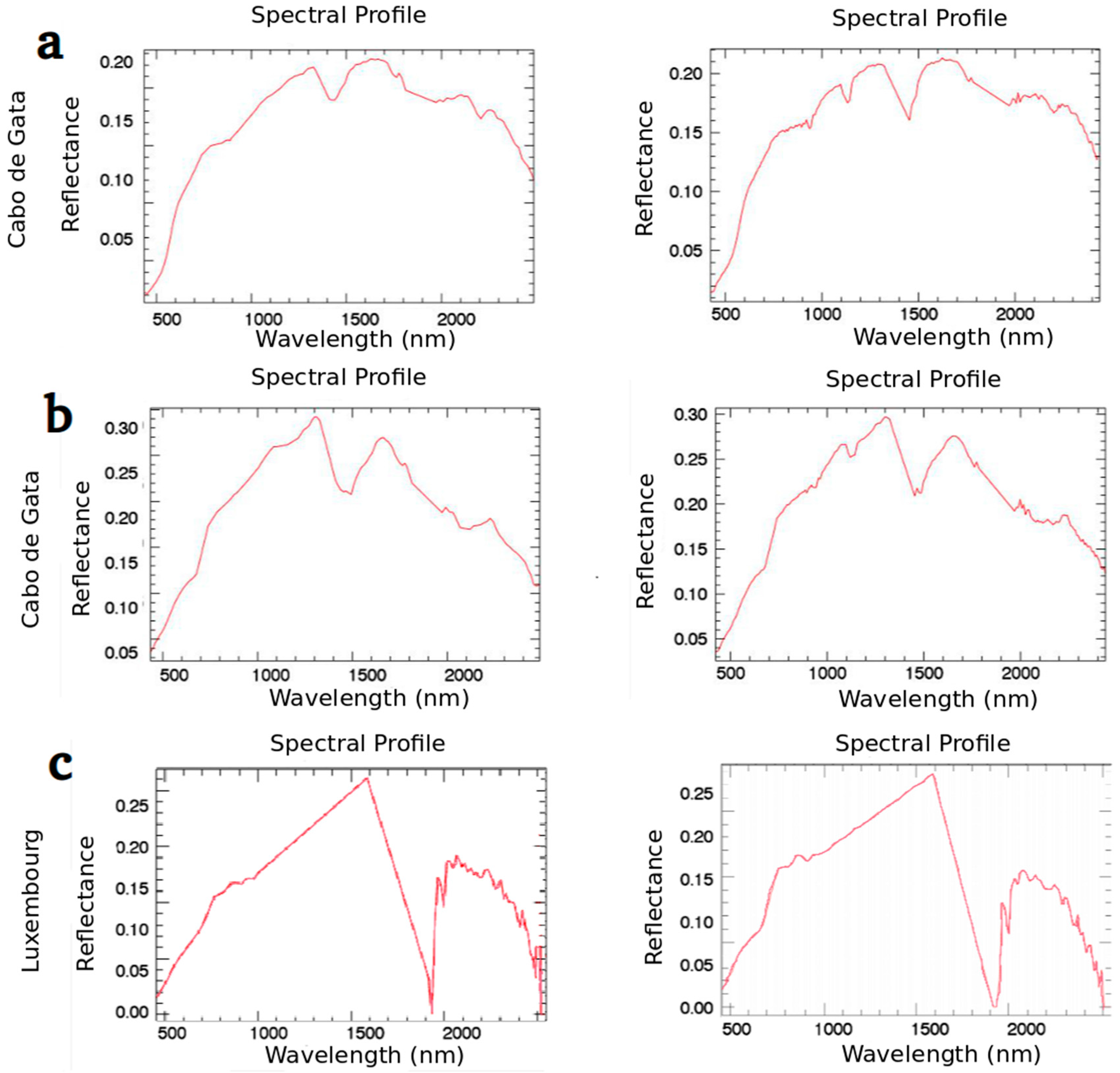
2.1. Test Sites and Datasets

Test sites were carefully selected based on: (1) the availability of high quality hyperspectral reflectance cubes in areas where bare soils are exposed; (2) the availability of extensive ground truth ground truth measurements including the soil properties iron oxide, clay, SOC, associated with surface sampling that have been acquired for validation of optical remote sensing imagery (top-surface samples, spatial sampling to cover homogeneous areas); (3) the presence of a high variability in the soil properties in question; and (4) the a priori feasibility of the spectral determination of a soil property from previous works in related areas. Two test sites were chosen, in Spain and in Luxembourg, in representative agricultural areas from two contrasting environments in semi-arid and temperate climatic zones. It is worth noting that the sampling strategy in both cases was conceptualized originally to accommodate the airborne scale of approximately 5 m × 5 m.

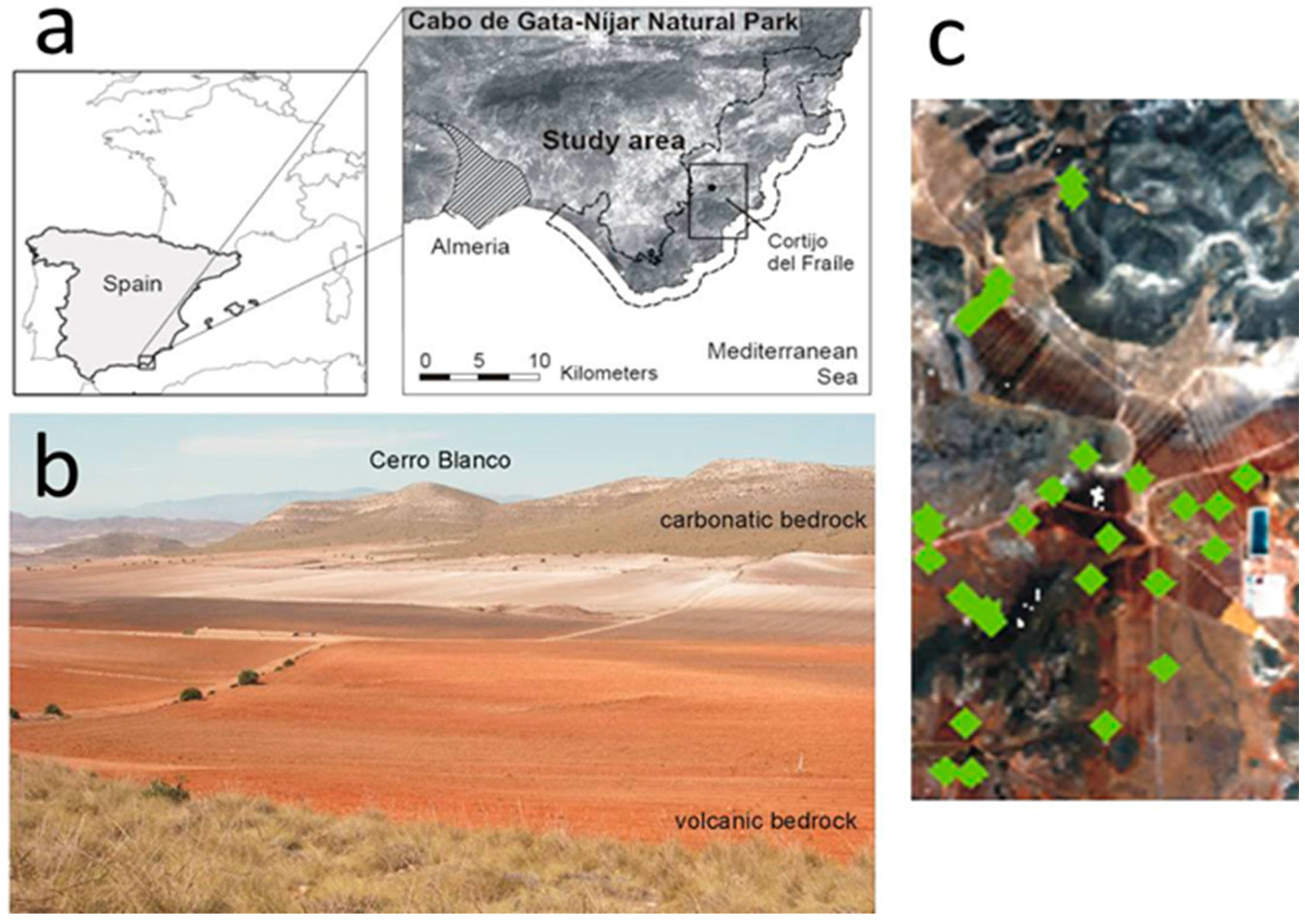
2.1.1. Cabo de Gata-Nijar Test Site for Iron Oxide and Clay Prediction

The first study area is located in the Natural Park Cabo de Gata-Níjar in the Almerian province of southeastern Spain, which is a semi-arid area with mean annual precipitation of 178 mm and mean annual temperature of 18.1 °C [37,38]. Our study focuses on a 6 km2 area at Cortijo del Fraile, which is an agricultural area in the middle of the park with mostly bare fields at the time of the overflight. The Park is characterized by two main geological units, one volcanic in the Southern part with high amounts of Fe-bearing minerals (e.g., hornblende, and biotite) [39], and the other sedimentary in the northern part consisting of marine limestones. An extensive ground truth validation dataset consisting of 51 field samples was characterized for iron oxide and clay content (Figure 1) [40,41]. Associated imaging spectroscopy data [42] were acquired over the area in June 2005 with the HyMap sensor from Integrated Spectronics Pty Ltd. (Baulkham Hills, NSW, Australia); http://www.hyvista.com), Australia. The HyMap sensor [43] provided spectral images after processing to geocoded reflectance with 126 contiguous spectral bands covering the spectral range of 400 to 2450 nm with a spectral resolution of 12 to 17 nm. The resulting ground sampling distance was 4.5 m for this dataset. Laboratory analysis of the field samples [41] showed a very high variability of soil chemical and textural properties. The iron oxide content measured as the citrate-dithionite extractable free iron oxide content (Fed) is normally distributed between 3.5 and 33.7 g·kg−1. The particle-size distribution ranged from sandy loam to clay and clay loam in the U.S. soil system, with a clay content varying between 8.4% and 63.4%.

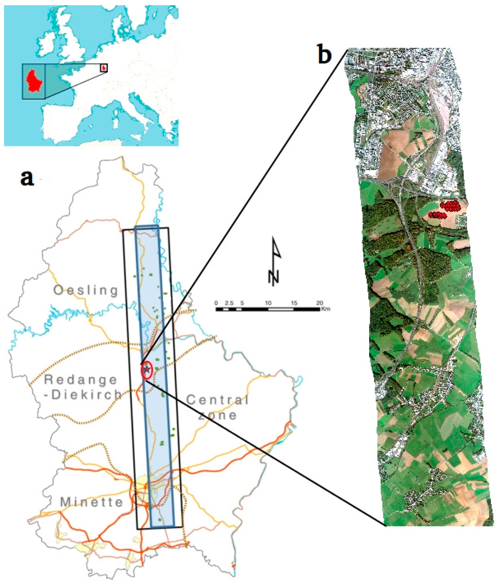
2.1.2. Luxembourg Test Site for SOC Prediction

For the validation of the SOC determination algorithm, a test site in the Grand-Duchy of Luxembourg was selected, where an extensive ground truth validation dataset of soil samples was collected in different bare fields [19]. Simultaneous, hyperspectral images were recorded over the test site area with the 80-band airborne hyperspectral Scanner AHS from INTA (www.inta.es), Madrid, Spain. The AHS-160 provided spectral images with 63 spectral bands from 450 to 2500 nm [44]. Due to a particular very low signal-to-noise ratio in the SWIR channels during data acquisition, this study focused on the VNIR part of the spectrum distributed on 20 contiguous spectral bands from 442 to 1019 nm with a spectral resolution between 27 and 30 nm. The resulting ground sampling distance was 2.6 m × 2.6 m. A total of 81 ground truth ground truth samples collected and measured for SOC out of the entirety of the samples from [19] associated with one AHS flight line covering ~7 km2 and representative of the variability in the region were found suitable for model calibration and validation (Figure 2). A high variability in SOC content ranging from 9 to 40 g·C·kg−1 was observed. Sand, sandy-loam and clay-loam soils exhibited a relatively low SOC variation and contained less than 25 g·C·kg−1 while clay, colluvial-alluvial and loam soils may contain up to 40 g·C·kg−1 and presented a large range of SOC contents in the calibration and validation dataset acquired.

2.1.3. Simulation of EnMAP Spaceborne Hyperspectral Images
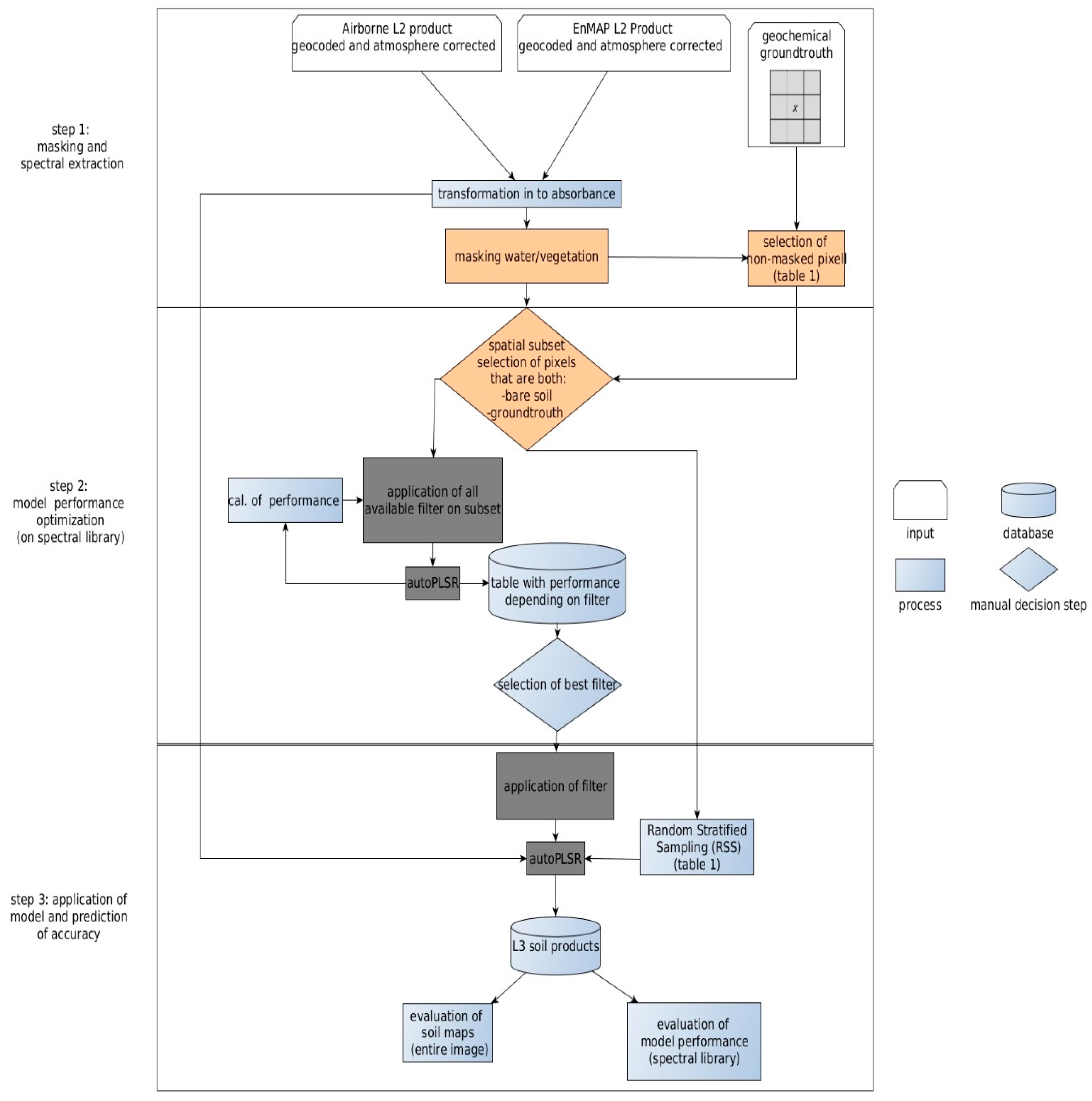
For each dataset, calculation of simulated EnMAP data and associated radiance and reflectance products (Level 1B/1C/2A) at 30 m resolution was performed using the EnMAP end-to-end simulation software EeteS [45]. The EeteS software follows the forward and backward processing schemes simulating the EnMAP image generation process, sensor calibration and data pre-processing. The core payload of EnMAP consists of a dual-spectrometer instrument measuring in 242 spectral bands between 420 and 2450 nm with a spectral sampling distance varying between 5 and 12 nm. It has a measured signal-to-noise ratio of 400:1 in the visible and near-infrared and 180:1 in the shortwave-infrared parts of the spectrum [45] that is considered in the EeteS sensor model. Sensor-like raw image data were produced using the airborne imagery and a digital elevation model (DEM) as input. Next, the data were transformed to Level 1C applying a detector co-registration and image orthorectification, then subsequently processed to reflectance orthorectified data (Level-2A) applying an atmospheric correction. Additional pre-processing of the reflectance simulated EnMAP imagery of the test sites included: (1) removal of the overlapping spectral channels between 900 to 1000 nm due to the two sensors overlap at this spectral region; and (2) removal of low signal-to-noise ratio spectral bands due to atmospheric attenuation around 1130, 1350 to 1500 and 1800 to 1950 nm, resulting in one spaceborne hyperspectral image cube for each test site with 212 spectral bands. Due to the lower spectral resolution of the HyMap and AHS sensor with regard to the EnMAP sensor, the EeteS simulation kept the original data spectral coverage (covering VNIR-SWIR for the Cabo de Gata data, and covering VNIR for the Luxembourg data), and introduced an interpolation of the data in the spectral dimension. Figure 3 presents a comparison of soil surface reflectance between airborne HyMAP/AHS imagery and spaceborne simulated EnMAP imagery in selected locations from field knowledge with high content of the soil properties studied. It can be observed that the spectral features observed in the soil airborne reflectance are maintained in the simulated EnMAP spectral signal. However, slight differences are observed mainly at noisy spectral regions in the EnMAP sensors associated with detectors edges (900 to 1000 nm) and at locations of atmospheric bands.

2.2. Methods

2.2.1. Quantitative Soil Prediction Models

For the multivariate modeling, the PLS approach was used to build prediction models based on available ground truth measurements. PLS models are widely used in hyperspectral remote sensing data analysis of soil properties (e.g., [19,22]) and are good in handling of situations with more predictors than observations [46]. The PLS regression projects predictors (X variables) and response (Y variable) into a low-dimensional space, i.e., a set of orthogonal variables called latent variables, maximizing the covariance between X- and Y-scores.
A detailed description of the PLS algorithm can be found in [46]. A Principal Component Analysis was run prior to the PLS, and for each spectrum the standardized Mahalanobis distance was calculated (H) to detect outliers with regard to the average spectrum [47]. Spectra with H greater than the square root of the 0.95 quantile of the chi-square distribution with two degrees of freedom were identified as outliers and excluded.
In this paper, we used the autoPLSR regression algorithms implemented in the EnMAP Box [48], deriving from the R package “autoPLSR” [49,50]. In order to avoid the problem of overfitting, a critical step of the PLS procedure is the determination of the appropriate number of latent variables. The great advantage of the autoPLSR approach lies in the non-expert, automatic, feature and latent variable selection that removes the need for manual fine-tuning. Better regression results could be expected by expert selection of latent variables and construction of a data specific feature space, as the PLS approach relies completely on the linear relationship between the feature space of latent variables and target variables as well as predictor variables. However, we used the autoPLSR as the operational ability is of interest here.
The autoPLSR software [49] is based on an iterative PLS approach, which uses an initial run, followed by automated predictor variable selection inside a tenfold cross-validation. Disregarding noisy, redundant and irrelevant variables, each iteration with the mentioned Mahalanobis distance criterion is followed up by re-runs, while creating each time predictor subsets, until no more reduction of model errors or latent vectors can be achieved or else the best model was selected. Predictor variables were scaled (centered to mean and normalized) beforehand. The same processing workflow was applied for both airborne and simulated EnMAP images and is presented in Figure 4. It can be separated into three major steps.
Step 1 included masking of non-bare soil pixels, transformation of reflectance (R) to absorbance log (1/R), and extraction of spectra for pre-autoPLSR regression runs.
Step 2 included a filter optimization utilizing a “fast” autoPLSR run only with a subset of data at selected ground truth locations. This is an iterative process that aimed at finding the best performing filter for the data by testing all reasonable pre-selected possibilities on a smaller subset of the data, and is part of the autoPLSR procedure.
Step 3 was associated with the main data processing where the selected best model for the PLS regression analysis was used and a final PLS equation was applied on the entire image. Subsequently, the PLS model performance was evaluated. A Random Stratified Selection (RSS) was applied for selection of calibration and validation dataset based on the ground truth data. A detailed description of each processing step is presented below. Software packages used also include the HYSOMA software [51] for soil masking and extraction of soil spectra from the image.

2.2.2. Pre-Processing

Pre-processing steps included a radiometric normalization to values between 0 and 1, and the calculation of absorbance log (1/R). Then, a mask was applied to the airborne and simulated EnMAP data cubes to keep pixels of bare soil surface only. The soil mask was created following the HYSOMA approach [51]: Open water surfaces were selected using the NDRBI (normalized difference red blue index), then the soil pixels were separated from green and dry matter vegetation components using the NDVI (normalized difference vegetation index) and the NCAI (normalized cellulose absorption index) based on pre-set threshold values. In addition, a mean filter was applied to the airborne data, so that the spectral signal of one pixel will be the average of 3 by 3 pixels. Then, image spectra were extracted that are associated with location of ground truth data. In the case of EnMAP simulated imagery, a single image spectrum was used and for airborne imagery the 3 by 3 window averaged image spectrum was used. Due to the coarser resolution of the EnMAP images, a visual examination of potential sample overlay was performed and potential duplicate samples (less than five samples in every case) were removed and only the ones closest to the center of the averaging window were used.

2.2.3. Model Building and Evaluation

The second step of our processing workflow involved finding the best performing filter in a fast performance test on a subset and subsequently applying the found filter and setting in the model building process on the entire image. The idea is to find the best pre-treatment to calibrate to the soil property to be predicted. This procedure was also done to account for the operational characteristics of this study.
In the fast performance test we applied the autoPLSR on smaller randomly selected square subsets (100 by 100 pixels) of the data, close to the center of the area of interest and including five data samples, of which three were used to construct the model and two to validate. We then evaluated the performance of this models built from the reduced dataset. This was run using different filters and degrees of filtering. As filter we considered the Savitzky–Golay smoothing and derivatives [52] or Gauss smoothing with fixed filter size. A fixed window width of five bands was used, making the absolute filter window width dependent on sensor spectral sampling and allowing different polynomial degrees (first to fifth degree) for the filter. The filter and its degree that performed best on the subset in this fast performance test were then applied to the entire image.
These operations aimed at decreasing the noise and enhancing possible spectral features linked to the property studied. The performance was evaluated using the RPIQ (ratio of performance to interquartile distance).
The next step was to build the final model with autoPLSR with the entire image dataset and the entire available ground truth samples up to this point. However, for the main run of autoPLSR, a calibration and validation dataset needed to be built from all the remaining available data samples. Finally, the autoPLSR was run with the calibration dataset and the smoothed image data.

2.2.4. Dataset Separation for Calibration and Validation

The third step was associated with the final run of the PLS model, derivation of the soil maps and calculation of the model performances. The ground truth dataset was separated to 60/40 by random stratified sampling (RSS) for which 60% of the data were used in the calibration dataset, and 40% for the validation. An exception was allowed here, however, permitting small deviations of ±10% from the 60/40 rule for each strata, if the centered mean of the calibration and validation datasets were of greater/smaller deviations than 20% of the standard mean deviation of the entire dataset, to ensure that a representative stack of data was selected for calibration and validation. This procedure led to small derivations from the 60%/40% calibration/validation distribution, but increased confidence in stability and representativeness of each subset.

2.2.5. Model Performance Assessment

Prediction performances of the regression models were assessed on the validation set and expressed by computing conventional performance indicators R2, Root Mean Square Error (RMSE), and RPD (ratio of performance deviation), all being dependent on the spread of the dataset and the shape of distribution. In addition, the RPIQ was computed as error measure. We made use of the RPD because it is an already established and well known error measure to which this study can be related to similar studies in the literature, but also made use of the RPIQ as RPIQ is a more robust and preferable way of standardizing the prediction error with respect to the spread of the population for soil analysis than RPD, as acknowledged by [53,54]. To produce the soil maps, the final PLS model was used to predict all non-masked pixels of the images, transformed with the automatically selected, best performing filters as given by the autoPLSR procedure.
Another measure of uncertainty was applied based on the variance model and calculations proposed by [55], which allows decomposing the total variance of estimated parameters into several contributors. It considers all sources of uncertainty, which affect the predictors, the dependent variables and the model coefficients. This variance modeling assumes that measurement errors have zero mean and that the error characteristics of the prediction objects are the same as the ones of the training objects. Four terms were used to describe and differentiate the variance contributors:
T1
the hyperspectral data uncertainty;
T2
the model coefficients uncertainty;
T3
the laboratory reference measurement uncertainty and sampling errors; and
T4
the dependency between the spectral and model uncertainties.

2.2.6. Spatial Structure Analysis and Influence of Sensor Resolution

Semivariogram analysis is a geostatistical method to quantify and model spatial dependence of attributes of interest. Semivariograms have been used in the context of soil science and in soil spectroscopy in several studies [25,33] as they provide information about spatial autocorrelation depending on sampling locations. In this study, semivariograms were applied to evaluate the resolvability of patterns of spatial structures in predicted soil properties between spaceborne (30 m) and airborne (4.5 and 2.6 m) images. As such, they complement the point-wise assessment of prediction accuracy. The parameters describing a semivariogram include nugget, sill and range [56]. It is assumed that nearby sample locations are spatially correlated, whereas locations further apart than the range are not correlated. A detailed introduction in semivariogram theory and semivariance formulas can be found in [56].
The generation of semivariograms was based on autoPLSR predicted soil map values in each pixel. A stepwise approach was applied, where first the semivariances were calculated and subsequently a simple linear regression was employed to find a good estimate of the semivariogram nugget. The nugget information is handed down, as well as the semivariances, to the next step, where Matérn model [57] based empirical semivariograms γ(h) of spherical geometry are built using a weighted least square fit, similar to [33].
The empirical semivariograms were computed based on bare soil pixels. For computational reasons, not all but a total of 6.25% of all bare soil pixels was selected in a random sampling, resulting in Cabo de Gata images in 29,490 and 9830 pixels for HyMAP and simulated EnMAP data, respectively, and for Luxembourg in 57,121 and 19,040 pixels for AHS and simulated EnMAP, respectively.

3. Results and Discussion

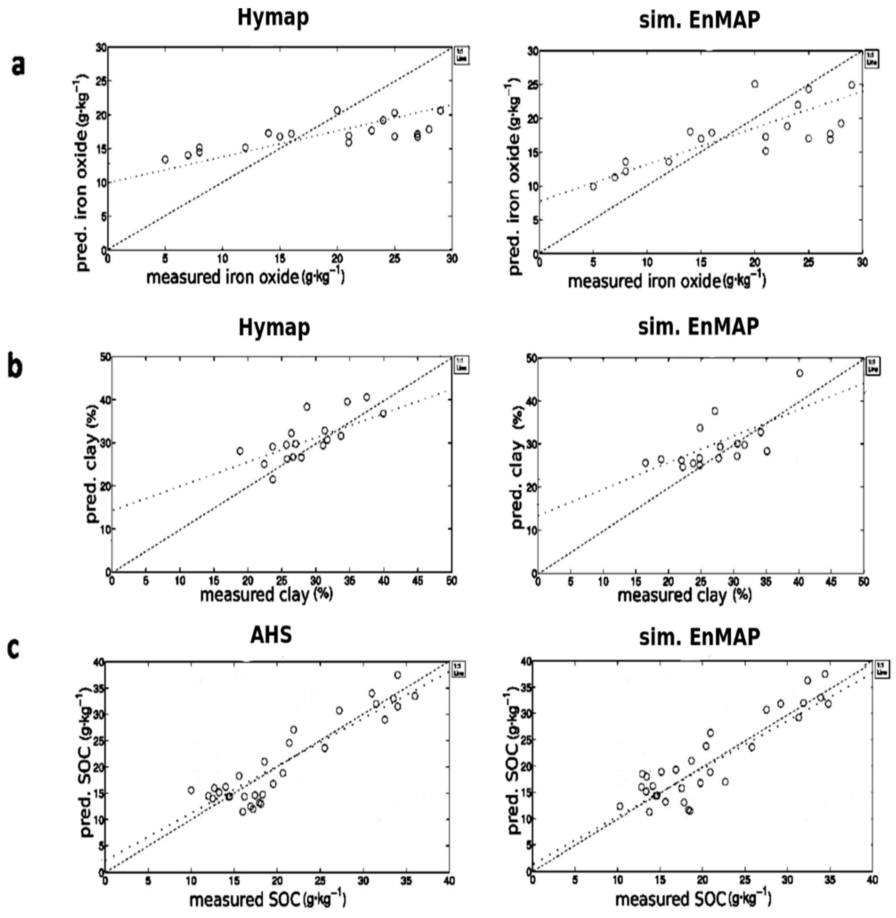
3.1. Quantitative Soil Prediction Models

After image pre-processing the number of ground truth samples available for model input at the spaceborne spatial scale was reduced by 4 for clay as compared to the airborne case, whereas it remained the same for the two other soil parameters (Table 1). The mean, lowest and maximum values of the soil parameters are given in Table 2.
For both, airborne and simulated EnMAP imagery, best pre-treatments were identified based on highest RPIQ values. The Savitzky–Golay smoothing transformation at the fifth order was always selected. This is consistent with [34], which found that the Savitzky–Golay algorithm consistently improved the ability of their models to predict SOC. Model performance statistics and regression plots were calculated (Table 3 and Figure 5).
RPIQ varies from ~1.4 (clay %, EnMAP) to ~2.9 (SOC g·kg−1, AHS). With the exception of the model for clay prediction from simulated EnMAP imagery, the RPIQ in all models is above 2.2; in addition, the RPIQ shows in all cases a conveying behavior between RMSE and R2, for example for the comparison of airborne iron oxide and clay. The iron oxide airborne performances have a R2 of 0.66 and a RMSE of 4.7. The results of the clay prediction model display a slightly lower R2 of 0.64 and RMSE of 2.4. The RPIQ of both cases is, however, comparable (2.3 and 2.2, respectively), showing an adaptive behavior to variance and performance evaluation of the RPIQ. In general, a slight decrease of model performances for EnMAP simulated imagery compared to airborne imagery is observed, linked to an irregular decrease in accuracy depending on test site and soil property studied. On the other hand, all RPD values are very similar and the performances of the models fall in an intermediate category (1.4 < RPD < 2), according to [58]. This was confirmed by R2 values in the validation set reaching 0.53–0.74. The decrease in model accuracy from airborne to spaceborne scale is relatively small (similar value or difference of 0.2% clay for RMSE) except for the SOC prediction (difference of 0.6 g·C·kg−1) where the airborne modeling at a smaller scale does perform much better than at the 30 m scale.
For the Cabo de Gata dataset, a previous study on iron oxide content mapping [59] applied an empirical modeling based on the physical analysis of the iron oxide absorption feature linked to the same airborne and ground truth dataset, which performed with an RPD of 2.19. A multivariate study of the area, based on Support Vector Machines [35], resulted in an RPD of 1.7. For Luxembourg, a previous soil airborne SOC study [19] found a comparable performance with the same dataset as well with RPD values in the same intermediate assessment category (between ~1.5 and ~2), depending on multivariate technique and spectral range. For a multivariate approach based on Support Vector Machines, a comparable, but slightly lower RPD of 1.6 was achieved in another study [35].
The uncertainty terms for the iron oxide parameters coincide with the uncertainties from [40,41]. For iron oxide from airborne data, the largest contribution to variance derives from the spectra (83%), followed by a mixture of all three components (9%), the model (5%) and finally the lab and presumably geostatistical errors (4%). The EnMAP variance contributors behave slightly different, i.e. the mixture term is higher at 12%, and the T3 also rises. The spectra term (T1) is lower with 75%. Clay, however, shows in comparison higher T3 error for airborne and EnMAP of 9% and 11%, respectively. SOC shows a similar pattern as iron oxide.
In general, the T1 term was identified as the main contributor to the variance in all cases (Table 4), with at least over 70% contribution. The term T3 is for EnMAP image based models always higher than for airborne based models in all three cases. In addition, the mixture term T4 is larger in all three cases, which is expected, if there is an inherent data base dependent performance change for example due to the resolution difference between scales. The modeling error T2, however, is comparable for all cases and parameters with no or only slight differences between airborne and EnMAP, showing a robustness of the model itself.
The resulting spatial distribution of the different soil properties is shown in Figure 6. In general, a coherent spatial distribution is observed between airborne and spaceborne imagery, although the lower spatial resolution of the EnMAP sensor at 30 m pixel scale is clearly visible.
The EnMAP soil maps display in each case a slightly higher mean value, as can be seen for example in the iron oxide prediction, while also showing lower maximum values in contrast to the HyMap/AHS soil mapping (see Table 2). The averaging effect of a larger pixel size might be responsible for this trend. On the other hand, for example, in the SOC prediction, EnMAP predicts generally lower SOC content in the southern fields in the image. The lowest predicted values of soil chemistry content in the EnMAP case in comparison to the airborne however show no clear trend. The red field in SOC EnMAP mapping is an artifact associated with an urban structure, which was not masked in the masking procedure.
Additionally, to be able to compare the spatial distribution, the airborne prediction results have been spatially resampled to fit the 30 m resolution scale of the simulated satellite data. Then, the Pearson coefficient of correlation was calculated for all pixels of the prediction results and all soil parameters studied. The results show between HyMAP/AHS and EnMAP predictions a good correlation for clay and SOC (0.86 and 0.84) and a very good correlation for iron oxide predictions (0.91).
The correlation in all cases is sufficient to support the validity of comparability for the EnMAP models to the airborne models.
The distribution of iron oxide and clay compared to a previous study [59] in the Cabo de Gata area show a very similar pattern, only the south of the area of interest shows lower values, where sampling was less dense than in other areas. The difference between the two might be due to differences in masking and soil modeling algorithms. The SOC distribution pattern is also comparable to a previous study in the Luxembourg area [19].

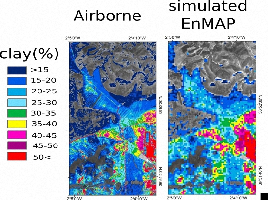
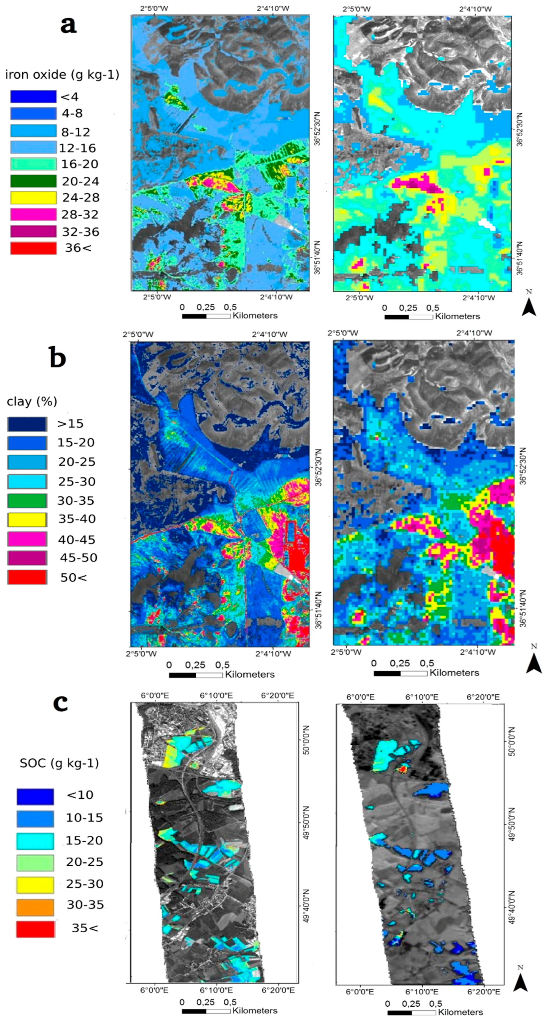
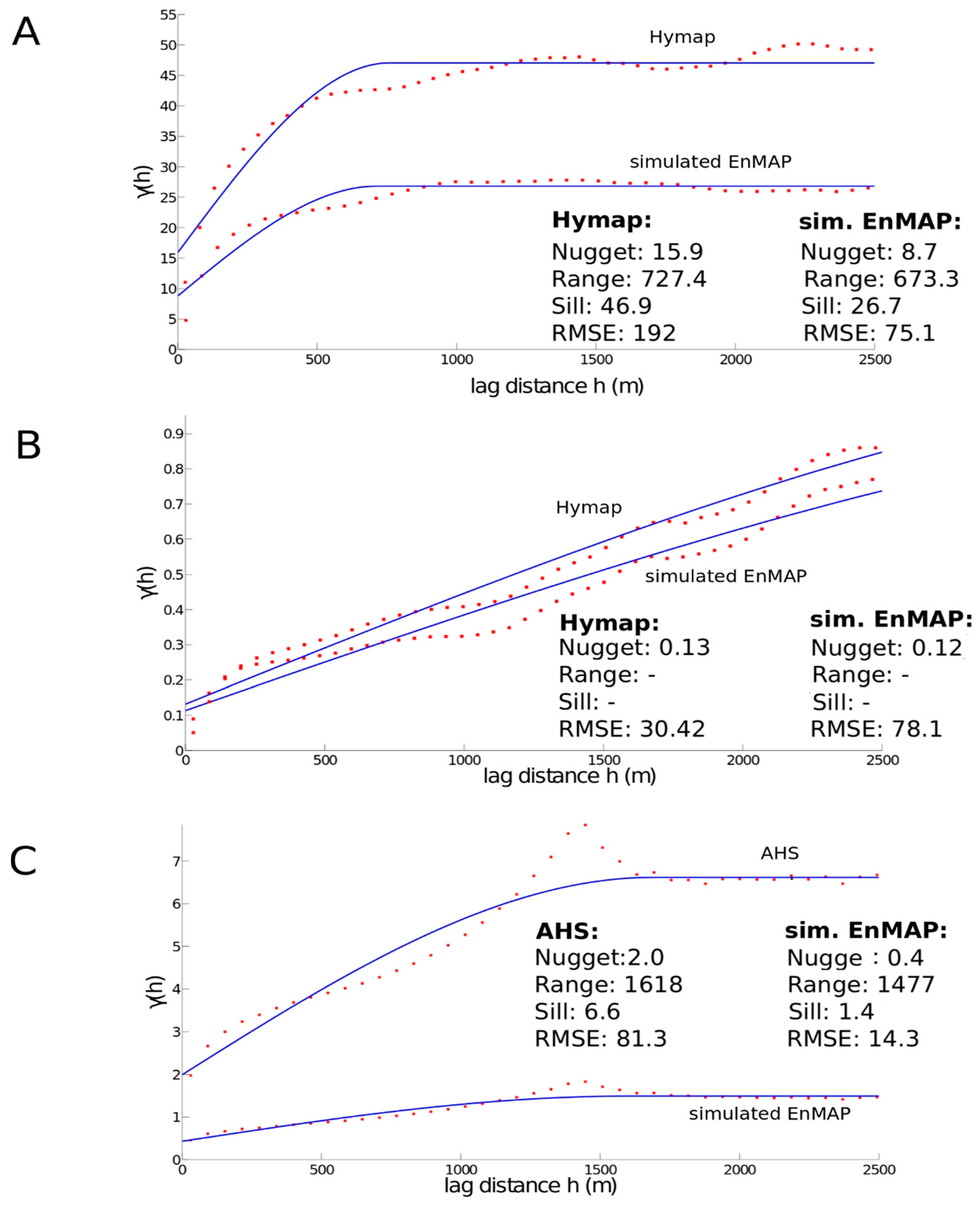
3.2. Spatial Structure Analysis and Influence of Sensor Resolution

In addition to the visual examination of the soil maps, the spatial structures of the predicted soil properties at airborne and spaceborne scale were compared using semivariograms. The fitted variograms based on the Matérn model along with the model parameters are shown in Figure 7. The maximum considered lag distance approximately corresponds to the east–west extent of the image data.
The empirical variograms (Figure 7) reveal variations in the range of approximately several hundred meters along distances likewise in the EnMAP and airborne based semivariances. The missing range and sill in Figure 7B is also discussed later. These may be attributed to the distribution of spatial units such as fields (in the case of Luxembourg) or geomorphic units (in the case of Cabo de Gata) with typical soil characteristics, while variance has not been calculated for large areas where pixels were masked out, so that the semivariograms are a direct representation of the geomorphological structures of the units of interest. Similar spatial variations were presented in other soil studies based on imaging spectroscopy [25,33,60]. In general, variograms calculated from image data are considered to represent the spatial structure of soil properties much better than regional variograms based on ground truth soil sampling [32]. Semivariance, nugget, range, sill and RMSE were found to always be lower for simulated EnMAP as compared to airborne images. This can be attributed to an averaging effect in predicted soil properties due to the lower spatial resolution, resulting in less extreme predicted values and a smoother increase of semivariance along distances based on EnMAP soil predictions. It is also underlined by the fact that the difference in semivariance between airborne and EnMAP is smaller for the Cabo de Gata dataset having 4.5 m pixel size than for the Luxembourg dataset having 2.6 m pixel size, or 13.5 m and 7.8, m respectively, taking the smoothing and averaging from preprocessing into account. Similarly, the predicted soil maps at airborne scale show a much finer spatial detail and short range variation in predicted soil properties.
The predicted iron content was found to have a nugget–sill ratio of 33.9% based on the airborne data and 32.6% based on the simulated EnMAP data. The ranges for predicted iron content expressing the lag distance where points are no longer spatially correlated were found to be 727 m (airborne) and 673 m (EnMAP). Predicted SOC showed nugget–sill ratios of 30.3% and 28.6%, respectively, and ranges of 1618 m and 1477 m, respectively. Nugget–sill ratios reported in the literature vary greatly depending on the local soil conditions and the sampling and analysis methods [32,61].
Generally, high nugget–sill values may be an indicator of discontinuity of the soil parameters or of an insufficient sampling not suitable to reproduce the distribution of the soil properties. In the studied case, the relatively high nugget–sill ratios suggest the presence of noise in the image data as stated by [60] that is propagated when simulating EnMAP data from airborne images. The ratio is also strongly affected by the performance of the soil prediction models and thus also by the soil sampling. In case of Cabo de Gata, most of the samples were collected in the topographically lower areas intersected by small ridges, while in the case of Luxembourg sampling points were located in a small area in the north east that may not be completely representative for the bare soil areas in the entire image.
The distribution of iron content in the Cabo de Gata site shows high values in the center of the area of interest and lower values further away from it resulting in a semivariogram with clearly defined range and sill. In the case of clay, however, sill and range values could not be obtained within the considered maximum lag distance. The clay content is distributed uneven in comparison to iron as it does not follow a natural distribution but is affected by strong anthropogenic influences with the presences of mining activities. This results in very high clay contents in the southeast corner of the area of interest in the mining area. Consequently, the spatial structure could not be captured in the semivariogram. The spatial distribution of SOC in Luxembourg is more homogeneous among fields than iron. In a single field, however, the higher values tend to be in the corners of the field for the airborne predictions, while the averaging effect of the higher EnMAP resolution is more visible for this parameter than for any other, leading to a strong flattening of the semivariograms fitting curve. The separation of mapped fields does not seem to influence the variogram.

4. Conclusions

Soil spectroscopy based on laboratory, field, and airborne data was shown to be an adequate method for the mapping of the spatial distribution of soil surface properties such as iron oxide, clay, and SOC content, moving into the quantitative domain based on multivariate statistics methodologies, as long as soil chromophores are present, the soils are well exposed and homogeneously distributed, and local ground data are available. In this paper, the potential of spaceborne spectroscopy data for the delivery of soil products is investigated. Nowadays, PLS approaches applied to soil spectroscopy have been recognized for its potential to deliver fast and low-cost high quality geo-referenced soil maps for the assessment of soil properties and for soil degradation indicators, and are used here.
With the upcoming launch of the next generation of imaging spectroscopy sensors (e.g., EnMAP, HISUI, HyspIRI, HypXIM, and SHALOM), a major step is expected towards global soil surface mapping from space using imaging spectroscopy. Nevertheless, in the frame of the preparation program for the EnMAP satellite mission to be launched in 2019 with more than 240 spectral bands covering the VNIR-SWIR at a pixel size of 30 m and a high signal-to-noise ratio, a central question at the forefront of research is the potential of the upcoming sensor system for surface soil properties mapping including the expected accuracy.
This paper presents a first study focusing on the test and validation of the EnMAP sensor for the quantitative spatial mapping of iron oxide, clay, and SOC content in semi-arid Mediterranean Spain and temperate area in Luxembourg. An emphasis is placed on the use of semi-operational method (autoPLSR approach in the EnMAP-Box), the evaluation of prediction accuracy, the use of conventional error measures but also uncertainty measures, and spatial structure analyses comparing airborne with spaceborne systems.
The overall results show that EnMAP data derived soil models are able to predict iron oxide, clay, and SOC with an R2 of the validation dataset between 0.53 and 0.67 compared to airborne imagery with R2 of the validation dataset between 0.64 and 0.74. The correlation between EnMAP and airborne imagery prediction results is in all cases higher than a Pearson coefficient of correlation of 0.86.
  • Although the slight decrease in prediction model performance, the spatial distribution of the soil properties is in general coherent between the simulated EnMAP and the airborne mapping.
  • The variance contributor analysis and semivariograms show a highlighted importance of resolution adapted sampling strategies for the simulated EnMAP case. Adapting to this can potentially increase the performance of future multivariate models.
  • The analyses of the variograms show that spatial structures predicted based on simulated EnMAP are well representative of the predicted spatial structures based on the airborne imagery with systematically lower calculated semivariance (averaging effect). The differences between EnMAP and airborne mapping are associated with heterogeneous areas where much finer detail and local variations are present in airborne soil maps and mixed pixels at EnMAP scale cannot represent variations at very small scale.
  • The shape of the semivariograms is coherent with local conditions for SOC and clay (crop fields, and geomorphic unit).
  • The automatic PLS procedure included in the EnMAP-Box is adequate to derive good soil prediction models which perform in an expected range (with RPIQ > 2.2 for the airborne data) and might be suitable for model building in an operational environment as long as adequate ground truth data are available.
  • This paper was a first example concerning case studies from two different soil environments using semi-operational multivariate statistics for the quantitative prediction of soil properties using simulated EnMAP satellite imagery. In general, this work demonstrates the high potential of upcoming spaceborne hyperspectral missions for soil science studies but has also shown the need for future adapted strategies to cope with the lower spatial resolution. Nevertheless, compared with airborne soil maps at much finer scale, simulated EnMAP images at 30 m scale with good spectral resolution and estimated signal-to-noise ratio similar to sensor tests were able to deliver regional soil maps that are coherent with previous analyses in the region.
  • Other factors that influence the prediction accuracy (e.g., spectral noise like atmosphere, surface roughness, sensor noise and illumination) are inherently included in error measures used and should be considered. We carried out a variance analysis to at least distinguish between modeling and data errors. The analysis showed that around 70%–80% of the variance of the results is due to uncertainties in the spectral data itself.
  • Further work should focus on the strategy to cope with degraded satellite signal compared to airborne hyperspectral imagery including field effects and the larger spatial resolution by developing adapted ground sampling strategies for independent validation of the soil models. In particular, more developments are needed on the methodological approaches to check the suitability of current and future improved soil algorithms for global soil mapping, and look at the availability of adequate methodologies for soil model building using appropriate databases for model calibration. One main avenue of research concerns the use of recently available regional and global soil spectral databases to calibrate the soil spectral models and further develop the capabilities for operational quantitative soil mapping from space.

Acknowledgments

The authors wish to thank Sibylle Itzerott for her continuous support for this study and funding of A. Steinberg. We thank Charly Kaufmann and Luis Guanter for support within the EnMAP science preparatory program funded under the DLR Space Administration with resources from the German Federal Ministry of Economic Affairs and Energy. Andreas Rabe from HU Berlin is gratefully acknowledged for technical support and helping with the EnMAP-Box and autoPLSR method. We acknowledge the University of Almeria and Paula Escribano for providing the Cabo de Gata soil data and Université Catholique de Louvain for providing the Luxembourg imagery and associated soil data.

Author Contributions

Andreas Steinberg, Sabine Chabrillat and Saskia Foerster conceived and designed the study and wrote the manuscript. Andreas Steinberg performed all analyses. Antoine Stevens provided the Luxembourg dataset and contributed to the manuscript writing. Karl Segl performed the EnMAP image simulations and revised the manuscript.

Conflicts of Interest

The authors declare no conflict of interest.

References

  1. Hartemink, A.E.; McBratney, A. A soil science renaissance. Geoderma 2008, 148, 123–129. [Google Scholar] [CrossRef]
  2. UNEP. UNEP Year Book 2012; United Nations Environment Program: Nairobi, Kenya, 2012. [Google Scholar]
  3. Grunwald, S.; Thompson, J.A.; Boettinger, J.L. Digital soil mapping and modeling at continental scales: Finding solutions for global issues. Soil Sci. Soc. Am. J. 2011, 75, 1201–1213. [Google Scholar] [CrossRef]
  4. Arrouays, D.; Grundy, M.G.; Hartemink, A.E.; Hempel, J.W.; Heuvelink, G.B.; Hong, S.Y.; Zhang, G.L. Chapter Three-GlobalSoilMap: Toward a fine-resolution global grid of soil properties. Adv. Agron. 2014, 125, 93–134. [Google Scholar]
  5. European Commission. Soil Protection—The Long Story Behind the Strategy; Office for Official Publications of the European Communities: Luxembourg, Luxembourg, 2006. [Google Scholar]
  6. Hunt, G.R. Spectral signatures of particulate minerals in the visible and near-infrared. Geophysics 1977, 42, 501–513. [Google Scholar] [CrossRef] [Green Version]
  7. Hunt, G.R.; Salisbury, J.W. Visible and near-infrared reflectance spectra of minerals and rocks, I: Silicate minerals. Mod. Geol. 1970, 1, 219–228. [Google Scholar]
  8. Ben-Dor, E.; Irons, J.R.; Epema, G.F. Soil reflectance. In Manual of Remote Sensing: Remote Sensing for the Earth Sciences, 3rd ed.; Wiley & Sons: New York, NY, USA, 1999; pp. 111–173. [Google Scholar]
  9. Chabrillat, S.; Pinet, P.C.; Ceuleneer, G.; Johnson, P.E.; Mustard, J.F. Ronda peridotite massif: Methodology for its geological mapping and lithological discrimination from hyperspectral data. Int. J. Remote Sens. 2000, 21, 2363–2388. [Google Scholar] [CrossRef]
  10. Ben-Dor, E.; Banin, A. Near-infrared analysis as a rapid method to simultaneously evaluate several soil properties. Soil Sci. Soc. Am. J. 1995, 59, 364–372. [Google Scholar] [CrossRef]
  11. Dalal, R.C.; Henry, R.J. Simultaneous determination of moisture, organic carbon, and total nitrogen by near infrared reflectance spectrophotometry. Soil Sci. Soc. Am. J. 1986, 50, 120–123. [Google Scholar] [CrossRef]
  12. Nocita, M.; Stevens, A.; Noon, C.; van Wesemael, B. Prediction of soil organic carbon for different levels of soil moisture using Vis-NIR spectroscopy. Geoderma 2013, 199, 37–42. [Google Scholar] [CrossRef]
  13. Sørensen, L.K.; Dalsgaard, S. Determination of clay and other soil properties by near infrared spectroscopy. Soil Sci. Soc. Am. J. 2005, 69, 159–167. [Google Scholar] [CrossRef]
  14. Bellon-Maurel, V.; McBratney, A. Near-infrared (NIR) and mid-infrared (MIR) spectroscopic techniques for assessing the amount of carbon stock in soils—Critical review and research perspectives. Soil Biol. Biochem. 2011, 43, 1398–1410. [Google Scholar] [CrossRef]
  15. Rossel, R.V.; Adamchuk, V.I.; Sudduth, K.A.; McKenzie, N.J.; Lobsey, C. Proximal soil sensing: An effective approach for soil measurements in space and time. Adv. Agron. 2011, 113, 243–291. [Google Scholar]
  16. Soriano-Disla, J.M.; Janik, L.J.; Viscarra Rossel, R.A.; Macdonald, L.M.; McLaughlin, M.J. The performance of visible, near-, and mid-infrared reflectance spectroscopy for prediction of soil physical, chemical, and biological properties. Appl. Spectrosc. Rev. 2014, 49, 139–186. [Google Scholar] [CrossRef]
  17. Nocita, M.; Stevens, A.; van Wesemael, B.; Aitkenhead, M.; Bachmann, M.; Barthes, B.; Ben Dor, E.; Brown, D.J.; Clairotte, M.; Csorba, A.; et al. Soil spectroscopy: An alternative to wet chemistry for soil monitoring. Adv. Agron. 2015, 132, 139–159. [Google Scholar]
  18. Ben-Dor, E.; Chabrillat, S.; Demattê, J.A.M.; Taylor, G.R.; Hill, J.; Whiting, M.L.; Sommer, S. Using imaging spectroscopy to study soil properties. Remote Sens. Environ. 2009, 113, S38–S55. [Google Scholar] [CrossRef]
  19. Stevens, A.; Udelhoven, T.; Denis, A.; Tychon, B.; Lioy, R.; Hoffmann, L.; van Wesemael, B. Measuring soil organic carbon in croplands at regional scale using airborne imaging spectroscopy. Geoderma 2010, 158, 32–45. [Google Scholar] [CrossRef]
  20. Gerighausen, H.; Menz, G.; Kaufmann, H. Spatially explicit estimation of clay and organic carbon content in agricultural soils using multi-annual imaging spectroscopy data. Appl. Environ. Soil Sci. 2012. [Google Scholar] [CrossRef]
  21. Bayer, A.; Bachmann, M.; Müller, A.; Kaufmann, H. A comparison of feature-based MLR and PLS regression techniques for the prediction of three soil constituents in a degraded South African ecosystem. Appl. Environ. Soil Sci. 2012. [Google Scholar] [CrossRef]
  22. Gomez, C.; Rossel, R.A.V.; McBratney, A.B. Soil organic carbon prediction by hyperspectral remote sensing and field Vis-NIR spectroscopy: An Australian case study. Geoderma 2008, 146, 403–411. [Google Scholar] [CrossRef]
  23. Gomez, C.; Lagacherie, P.; Coulouma, G. Continuum removal versus PLSR method for clay and calcium carbonate content estimation from laboratory and airborne hyperspectral measurements. Geoderma 2008, 148, 141–148. [Google Scholar] [CrossRef]
  24. Stevens, A.; Nocita, M.; Toth, G.; Montanarella, L.; van Wesemael, B. Prediction of soil organic carbon at the European scale by visible and NearInfraRed reflectance spectroscopy. PLoS ONE 2013, 8, e66409. [Google Scholar] [CrossRef] [PubMed]
  25. Gomez, C.; Lagacherie, P.; Coulouma, G. Regional predictions of eight common soil properties and their spatial structures from hyperspectral Vis-NIR data. Geoderma 2012, 189, 176–185. [Google Scholar] [CrossRef]
  26. Guanter, L.; Kaufmann, H.; Segl, K.; Förster, S.; Rogaß, C.; Chabrillat, S.; Küster, T.; Hollstein, A.; Rossner, G.; Chlebek, C.; et al. The EnMAP spaceborne imaging spectroscopy mission for earth observation. Remote Sens. 2015, 7, 8830–8857. [Google Scholar] [CrossRef]
  27. Vågen, T.-G.; Leigh, A.; Winowiecki, A.; Tondoh, J.E.; Desta, L.T.; Gumbricht, T. Mapping of soil properties and land degradation risk in Africa using MODIS reflectance. Geoderma 2016, 263, 216–225. [Google Scholar] [CrossRef]
  28. Cudahy, T.; Caccetta, M.; Lau, I.; Rodger, A.; Laukamp, C.; Ong, C.; Chia, J.; Collings, S.; Rankine, T.; et al. Satellite ASTER geoscience map of Australia. v1. CSIRO. Data Collect. 2012. [Google Scholar] [CrossRef]
  29. Okujeni, A.; van der Linden, S.; Hostert, P. Extending the vegetation-impervious-soil model using simulated EnMAP data and machine learning. Remote Sens. Environ. 2015, 158, 69–80. [Google Scholar] [CrossRef]
  30. Malec, S.; Rogge, D.; Heiden, U.; Sanchez-Azofeifa, A.; Bachmann, M.; Wegmann, M. Capability of spaceborne hyperspectral EnMAP mission for mapping fractional cover for soil erosion modeling. Remote Sens. 2015, 7, 11776–11800. [Google Scholar] [CrossRef]
  31. Gomez, C.; Oltra-Carrió, R.; Bacha, S.; Lagacherie, P.; Briottet, X. Evaluating the sensitivity of clay content prediction to atmospheric effects and degradation of image spatial resolution using hyperspectral VNIR/SWIR imagery. Remote Sens. Environ. 2015, 164, 1–15. [Google Scholar] [CrossRef]
  32. Mulder, V.L.; de Bruina, S.; Weyermann, J.; Kokaly, R.F.; Schaepman, M.E. Characterizing regional soil mineral composition using spectroscopy and geostatistics. Remote Sens. Environ. 2013, 139, 415–429. [Google Scholar] [CrossRef]
  33. Schwanghart, W.; Jarmer, T. Linking spatial patterns of soil organic carbon to topography: A case study from south-eastern Spain. Geomorphology 2011, 126, 252–263. [Google Scholar] [CrossRef]
  34. Vasques, G.M.; Grunwald, S.J.O.S.; Sickman, J.O. Comparison of multivariate methods for inferential modeling of soil carbon using visible/near-infrared spectra. Geoderma 2008, 146, 14–25. [Google Scholar] [CrossRef]
  35. Chabrillat, S.; Foerster, S.; Steinberg, A.; Segl, K. Prediction of common surface soil properties using airborne and simulated EnMAP hyperspectral images: Impact of soil algorithm and sensor characteristic. In Proceedings of the 2014 IEEE International Geoscience and Remote Sensing Symposium, Québec City, QC, Canada, 13–18 July 2014; pp. 2914–2917.
  36. Guerrero, C.; Stenberg, B.; Wetterlind, J.; Viscarra Rossel, R.A.; Maestre, F.T.; Mouazen, A.M.; Zornoza, R.; Ruiz-Sinoga, J.D.; Kuang, B. Assessment of soil organic carbon at local scale with spiked NIR calibrations: Effects of selection and extra-weighting on the spiking subset. Eur. J. Soil Sci. 2014, 65, 248–263. [Google Scholar] [CrossRef]
  37. Aranda, V.; Oyonarte, C. Effect of vegetation with different evolution degree on soil organic matter in a semi-arid environment (Cabo de Gata-Níjar Natural Park, SE Spain). J. Arid Environ. 2005, 62, 631–647. [Google Scholar] [CrossRef]
  38. Paruelo, J.M.; Piñeiro, G.; Escribano, P.; Oyonarte, C.; Alcaraz, D.; Cabello, J. Temporal and spatial patterns of ecosystem functioning in protected arid areas in southeastern Spain. Appl. Veg. Sci. 2005, 8, 93–102. [Google Scholar] [CrossRef]
  39. Fernández-Soler, J.M. Volcanics of the Almeria province. A field guide to the Neogene sedimentary basins of the Almería province. SE Spain 2001, 7, 58–88. [Google Scholar]
  40. Richter, N.; Chabrillat, S.; Kaufmann, H. Enhanced quantification of soil variables linked with soil degradation using imaging spectroscopy. In Proceedings of the 5th EARSeL Workshop, Bruges, Belgium, 23–25 April 2007; p. 7.
  41. Richter, N.; Jarmer, T.; Chabrillat, S.; Oyonarte, C.; Hostert, P.; Kaufmann, H. Free iron oxide determination in Mediterranean soils using diffuse reflectance spectroscopy. Soil Sci. Soc. Am. J. 2009, 73, 72–81. [Google Scholar] [CrossRef]
  42. Chabrillat, S.; Naumann, N.; Escribano, P.; Bachmann, M.; Spengler, D.; Holzwarth, S.; Palacios-Orueta, A.; Oyonarte, C. Cabo de Gata-Nίjar natural park 2003–2005—A multitemporal hyperspectral flight campaign for EnMAP science preparatory activities. EnMAP flight campaigns technical report. GFZ Data Serv. 2016. [Google Scholar] [CrossRef]
  43. Cocks, T.; Jenssen, R.; Steward, A.; Wilson, I.; Shields, T. The HyMap airborne hyperspectral sensor: The system, calibration and performance. In Proceedings of the 1st European Association of Remote Sensing Laboratories (EARSeL) Workshop on Imaging Spectroscopy, University of Zurich, Switzerland, 6–8 October 1998; pp. 37–42.
  44. Fernández-Renau, A.; Gómez, J.A.; de Miguel, E. The INTA AHS system. Proc. SPIE 2005. [Google Scholar] [CrossRef]
  45. Segl, K.; Guanter, L.; Rogaß, C.; Küster, T.; Roessner, S.; Kaufmann, H.; Sang, B.; Mogulsky, V.; Hofer, S. EeteS—The EnMAP end-to-end simulation tool. IEEE J. Sel. Top. Appl. Earth Obs. Remote Sens. 2012, 5, 522–530. [Google Scholar] [CrossRef]
  46. Wold, S.; Sjöström, M.; Eriksson, L. PLS-regression: A basic tool of chemometrics. Chemom. Intell. Lab. Syst. 2001, 58, 109–130. [Google Scholar] [CrossRef]
  47. Mark Howard, L.; Tunnell, D. Qualitative near-infrared reflectance analysis using Mahalanobis distances. Anal. Chem. 1985, 57, 1449–1456. [Google Scholar] [CrossRef]
  48. Van der Linden, S.; Rabe, A.; Held, M.; Jakimow, B.; Leitão, P.J.; Okujeni, A.; Schwieder, M.; Suess, S.; Hostert, P. The EnMAP-Box—A toolbox and application programming interface for EnMAP data processing. Remote Sens. 2015, 7, 11249–11266. [Google Scholar] [CrossRef]
  49. Oldenburg, C.; Schmidtlein, S.; Feilhauer, H. AutoPLSR: Manual for Application: AutoPLSR (1.x), EnMAP-Box Documentation. Available online: http://www.dev.geo.hu-berlin.de/enmap-box/documentation/applications/autoPLSR/help/manual.pdf (accessed on 12 August 2015).
  50. Schmidtlein, S.; Bruelheide, H.; Feilhauer, H. Mapping plant strategy types using remote sensing. J. Veg. Sci. 2012, 23, 395–604. [Google Scholar] [CrossRef]
  51. Chabrillat, S.; Eisele, A.; Guillaso, S.; Rogaß, C.; Ben-Dor, E.; Kaufmann, H. HYSOMA: An easy-to-use software interface for soil mapping applications of hyperspectral imagery. In Proceedings of the 7th EARSeL SIG Imaging Spectroscopy Workshop, Edinburgh, UK, 11–13 April 2011.
  52. Savitzky, A.; Golay, M.J. Smoothing and differentiation of data by simplified least squares procedures. Anal. Chem. 1964, 36, 1627–1639. [Google Scholar] [CrossRef]
  53. Bellon-Maurel, V.; Fernandez-Ahumada, E.; Palagos, P.; Roger, J.-M.; McBratney, A.B. Critical review of chemometric indicators commonly used for assessing the quality of the prediction of soil attributes by NIR spectroscopy. TrAC Trends Anal. Chem. 2010, 29, 1073–1081. [Google Scholar] [CrossRef]
  54. Sarkhot, D.V.; Grunwald, S.; Ge, Y.; Morgan, C.L.S. Comparison and detection of total and available soil carbon fractions using visible/near infrared diffuse reflectance spectroscopy. Geoderma 2011, 164, 22–32. [Google Scholar] [CrossRef]
  55. Fernandez-Ahumada, E.; Roger, J.M.; Palagos, B. A new formulation to estimate the variance of model prediction. Application to near infrared spectroscopy calibration. Anal. Chim. Acta 2012, 721, 28–34. [Google Scholar] [CrossRef] [PubMed]
  56. Wackernagel, H. Multivariate Geostatistics: An Introduction with Applications; Springer Science & Business Media: Berlin, Germany, 2013. [Google Scholar]
  57. Matérn, B. Spatial variation, meddelanden fran statens skogsforskningsinstitut. Lect. Notes Stat. 1960, 36, 21. [Google Scholar]
  58. Chang, C.-W.; Laird, D.A.; Mausbach, M.J.; Hurburgh, C.R. Near-infrared reflectance spectroscopy—Principal components regression analyses of soil properties. Soil Sci. Soc. Am. J. 2001, 65, 480–490. [Google Scholar] [CrossRef]
  59. Richter, N. Pedogenic Iron Oxide Determination of Soil Surfaces from Laboratory Spectroscopy and HyMap Image Data—A Case Study in Cabo de Gata-Nijar Natural Park. Ph.D. Thesis, Mathematisch-Naturwissenschafltichen Fakultät II der Humboldt-Universität, Berlin, Germany, 2009. [Google Scholar]
  60. Rousseeuw, P.J.; Debruyne, M.; Engelen, S.; Hubert, M. Robustness and outlier detection in chemometrics. Crit. Rev. Anal. Chem. 2006, 36, 221–242. [Google Scholar] [CrossRef]
  61. Odlare, M.; Svensson, K.; Pell, M. Near infrared reflectance spectroscopy for assessment of spatial soil variation in an agricultural field. Geoderma 2005, 126, 193–202. [Google Scholar] [CrossRef]
Figure 1. Cabo de Gata-Nijar Natural Park test site (modified from [40]): (a) map of Spain with location of HyMap imagery (bold rectangle) and study area Cortijo del Fraile; (b) wiew of the volcanic-carbonatic bedrock transition; and (c) RGB true-color HyMap imagery with sample points (green dots) and selected study area Cortijo del Fraile.
Remotesensing 08 00613 g001
Figure 2. Luxembourg test site (modified from [19]). (a) Top: Map of Europe with location of Luxembourg; Bottom: Map of the Grand-Duchy of Luxembourg with sampling points (dots), selected flight line (blue rectangle); (b) RGB true-color AHS imagery and location of samples points (red dots).
Remotesensing 08 00613 g002
Figure 3. Soil spectral reflectance from airborne HyMAP and AHS (left) and spaceborne simulated EnMAP (right) imagery at: (a) Cabo de Gata iron-rich and clay-rich bare field area; (b) Cabo de Gata dry vegetation area; and (c) Luxembourg bare field area.
Remotesensing 08 00613 g003
Figure 4. Work flow of soil prediction modeling in this study. Grey shaded boxes indicate use of the EnMAP toolbox and light color boxes the use of the Hysoma toolbox, while blue boxes indicate steps developed uniquely in this study.
Remotesensing 08 00613 g004
Figure 5. Plots of measured vs. predicted soil parameters for the validation datasets as obtained: (a) Iron oxide content (g·kg−1), Cabo de Gata test site; (b) Clay content (%), Cabo de Gata test site; NS (c) SOC content (g·kg−1), Luxembourg test site. Left: Airborne imagery (a,b) HyMAP (4.5 m) and (c) AHS (2.6 m); Right: Spaceborne simulated EnMAP images (30 m).
Remotesensing 08 00613 g005
Figure 6. Maps of predicted soil properties: (a) Iron oxide, Cabo de Gata test site; (b) Clay content, Cabo de Gata test site; and (c) SOC content, Luxembourg test site. Left: Airborne imagery (a,b) HyMAP (4.5 m); and (c) AHS (2.6 m). Right: Spaceborne simulated EnMAP images (30 m).
Remotesensing 08 00613 g006
Figure 7. Semivariograms for: (A) Iron oxide, Cabo de Gata test site; (B) Clay, Cabo de Gata test site; and (C) SOC content, Luxembourg test site. The descriptive parameters are included in the figure. RMSE is given in m. γ(h) is the semivariance, which is also given in m.
Remotesensing 08 00613 g007
Table 1. Available ground truth soil database: Total number of samples available, and resulting number of soil samples selected for calibration/validation, as derived from selection of bare pixels and random stratified sampling.
Soil Database AvailableSelected HyMap/AHSSelected EnMAP
Iron Oxide5123/2023/20
Clay5125/1822/17
SOC8146/3146/31
Table 2. Mean, minimum and maximum values of iron oxide (g·kg−1), clay (%) and SOC (g·kg−1) from the derived soil products.
Iron OxideClaySOC
HyMap/AHS14.3 (3.7, 41.5)20.1 (7.7, 65.3)14.6 (8.9, 42.6)
EnMAP14.3 (3.7, 41.2)21.9 (7.9, 65.1)14.9 (8.2, 41.1)
Table 3. Model performance statistics for the validation dataset was calculated and regression plots are depicted in (a) (HyMap/AHS) and (b) (simulated EnMAP). Top: Iron oxide content Cabo de Gata test site; Middle: clay content Cabo de Gata test site, Bottom: SOC content Luxembourg test site. * relates to different units of RMSE depending on the soil properties considered: RMSE is given in g·kg−1 for iron oxide and SOC, RMSE is given in % for clay.
(a) Airborne HyMap/AHS
R2RMSE *RPDRPIQ
Iron Oxide0.664.71.72.3
Clay0.642.41.72.2
SOC0.742.21.92.9
(b) Spaceborne EnMAP
R2RMSE *RPDRPIQ
Iron Oxide0.651.62.2
Clay0.532.61.51.4
SOC0.672.81.72.2
Table 4. Values of uncertainty expressions for (a) airborne HyMap/AHS imagery; and (b) simulated EnMAP images. The values are relative (in %) to the total variance. The terms are: T1 the hyperspectral data uncertainty, T2 the model coefficients uncertainty, T3 the laboratory reference measurement uncertainty, and T4 the dependency between the spectral and model uncertainties (mixture term).
(a) HyMap/AHS
T1T2T3T4
Iron Oxide0.830.050.040.09
Clay0.760.060.090.10
SOC0.800.050.040.11
(b) EnMAP
T1T2T3T4
Iron Oxide0.750.050.080.12
Clay0.700.060.130.11
SOC0.720.600.090.13

