Article

Sea and Freshwater Ice Concentration from VIIRS on Suomi NPP and the Future JPSS Satellites

1
Cooperative Institute for Meteorological Satellite Studies, University of Wisconsin-Madison, 1225 West Dayton St., Madison, WI 53706, USA
2
NOAA/NESDIS, 1225 West Dayton St., Madison, WI 53706, USA
3
Northrop Grumman Aerospace Systems, Redondo Beach, CA 90278, USA
*
Author to whom correspondence should be addressed.
Remote Sens. 2016, 8(6), 523; https://doi.org/10.3390/rs8060523
Submission received: 9 March 2016 / Revised: 1 June 2016 / Accepted: 13 June 2016 / Published: 22 June 2016
(This article belongs to the Special Issue Sea Ice Remote Sensing and Analysis)

Abstract

:
Information on ice is important for shipping, weather forecasting, and climate monitoring. Historically, ice cover has been detected and ice concentration has been measured using relatively low-resolution space-based passive microwave data. This study presents an algorithm to detect ice and estimate ice concentration in clear-sky areas over the ocean and inland lakes and rivers using high-resolution data from the Visible Infrared Imaging Radiometer Suite (VIIRS) onboard the Suomi National Polar Orbiting Partnership (S-NPP) and on future Joint Polar Satellite System (JPSS) satellites, providing spatial detail that cannot be obtained with passive microwave data. A threshold method is employed with visible and infrared observations to identify ice, then a tie-point algorithm is used to determine the representative reflectance/temperature of pure ice, estimate the ice concentration, and refine the ice cover mask. The VIIRS ice concentration is validated using observations from Landsat 8. Results show that VIIRS has an overall bias of −0.3% compared to Landsat 8 ice concentration, with a precision (uncertainty) of 9.5%. Biases and precision values for different ice concentration subranges from 0% to 100% can be larger.

Graphical Abstract

1. Introduction

Observations of ice cover and ice concentration—the fraction of an area covered by ice—are important for commercial transportation, short-term weather forecasting, water management, and damage control, and climate change studies. Arctic sea ice has changed dramatically in the past few decades [1]. Sea ice extent has been decreasing significantly [2], associated with changes in sea ice thickness and age [3,4]. Sea ice in the Antarctic has also been changing, with positive trends in sea ice extent and area [5]. Sea ice interacts with other physical components in the polar climate system. Studies have linked the shrinking of summer/fall sea ice with surface warming [6], a less stable lower troposphere [7], increased cloud amount [8,9], mid-latitude weather and extreme events through teleconnection between Arctic and mid-latitude [10,11,12], and other changes [13].
Sea ice products using satellite observations in the microwave portion of the electromagnetic spectrum have been used for decades. Several widely used sea ice algorithms are the NASA Team (NT) algorithm [14], the enhanced NT algorithm [15], the Bootstrap (BS) algorithm [16], and the ARTIST Sea Ice (ASI) algorithm [17]. More details on the microwave sea ice products can be found in [18,19] and references therein. Advantages of passive microwave data include its high temporal coverage and all weather capability. However, the spatial resolutions of these data sets are relatively coarse. For example, sea ice concentration (SIC) products at a grid cell size of 25 km × 25 km from the scanning multichannel microwave radiometer (SMMR) onboard the Nimbus-7 satellite, the Special Sensor Microwave/Imager (SSMI) onboard the Defense Meteorological Satellite Program (DMSP) F8, F11, and F13 platforms, and the Special Sensor Microwave Imager Sounder (SSMIS) onboard the DMSP F17 platform [20,21] are the most common products. Ice products using the Advanced Microwave Scanning Radiometer—Earth Observing System (AMSR-E) onboard the Aqua satellite and the Advanced Microwave Scanning Radiometer 2 (AMSR2) onboard the Global Change Observation Mission 1st (GCOM-W1) satellite can have higher spatial resolution [22,23]. This spatial resolution may be satisfactory for climate studies, but may not be adequate for navigation and small-scale studies of ice dynamics and meteorology. Active microwave observations, e.g., space-borne synthetic aperture radar (SAR), can make an important contribution to sea ice concentration retrieval and sea ice monitoring with its high resolution and all-sky capability [24,25].
Visible and infrared (hereafter “visible/IR”) data provide the possibility of higher spatial resolution ice concentration products, with the shortcoming that they are only available under clear-sky conditions. Visible/IR data may also produce more accurate summertime ice concentrations, which are difficult to obtain with passive microwave data due to the similar emissivities of melt ponds and open water. The shortcoming of the ice concentration from visible data is that they are only available in the daytime. Methods have been developed to estimate ice concentration from visible/IR imagers such as the Advanced Very High Resolution Radiometer (AVHRR), the Moderate Resolution Imaging Spectroradiometer (MODIS), and the Visible Infrared Imaging Radiometer Suite (VIIRS) [26,27,28,29,30,31,32]. VIIRS, which is currently onboard the Suomi National Polar Orbiting Partnership (S-NPP) satellite and will fly on future Joint Polar Satellite System (JPSS) satellites, provides an opportunity to better monitor the ice routinely due to its high spatial resolution, better signal-to-noise ratio, and a wider swath than its heritage sensors [33]. In addition, the combination of VIIRS and MODIS will provide a long time series of ice information that can be used to study the role of ice in the climate system.
Here, we present an algorithm that will be used operationally by the U.S. National Oceanic and Atmospheric Administration (NOAA) to generate ice cover mask and ice concentration products over the oceans, lakes, and rivers from JPSS VIIRS. It is also being implemented for S-NPP VIIRS, to run in parallel with the current operational product that is generated by the NOAA Interface Data Processing Segment (IDPS). This new algorithm, one of NOAA’s “Enterprise” algorithms, was first developed for use with the future Geostationary Operational Environmental Satellite-R (GOES-R) Advanced Baseline Imager. It builds on previous algorithms developed for AVHRR, MODIS, and VIIRS, notably the IDPS ice concentration algorithm [34]. The methodology is applied to sea ice in the Arctic Ocean and freshwater ice in the Great Lakes. Also presented is a robust examination of the product accuracy using high-resolution visible/IR imagery from Landsat 8. A comparison to ice concentration derived from low-resolution passive microwave SSMIS and AMSR2 data provides a useful perspective on the difficulties of validating ice concentration products.

2. Data and Method

A high level processing flow diagram illustrates the main processing sections of the ice cover mask and ice concentration algorithm (Figure 1). Details of input data and methods are explained in this section.

2.1. Algorithm Data Input

2.1.1. Instrument Input

S-NPP was launched on 28 October 2011. S-NPP is a polar orbiting satellite with an early afternoon ascending equator crossing time of 1:30 p.m. local time. S-NPP orbits the polar regions 14 times a day and provides complete coverage of the polar regions twice daily. VIIRS has 22 spectral bands covering wavelengths from 0.4 to 11.8 μm. Of the 22 bands, there are five high resolution imagery bands (the “I” bands, 375 m spatial resolution at nadir), 16 moderate resolution bands (“M” bands, 750 m spatial resolution at nadir), and one Day/Night Band (DNB, 750 m spatial resolution). The VIIRS swath width is 3000 km. The VIIRS reflective solar band radiometric uncertainties are within 2% [33]. The horizontal sampling interval at the scan edge grows by a factor of two compared to nadir, which results in a bow-tie effect. VIIRS applies bow-tie deletion to remove duplicated pixels in the off-nadir part of the scan [33,34]. The geolocation error for the I and M bands is around 1% of the pixel size in mean and less than 20% of the pixel size in root mean squared error [35].
Inputs to the ice concentration algorithm include reflectances at 0.67 μm, 0.86 μm, 1.6 μm at the top of the atmosphere (TOA) without a solar zenith angle correction, and split-window brightness temperatures at 10.7 and 11.8 μm (more generally referred to as 11 and 12 μm), which are VIIRS band M5, M7, M10, M15, and M16 (Table 1). Inputs also include geolocation, solar zenith angle, and satellite zenith angle.

2.1.2. Derived Products

A cloud mask and a clear-sky ice surface temperature product are also used. The current S-NPP VIIRs cloud mask is derived using multiple threshold methods [36]. For future JPSS satellites, a Bayesian cloud mask will be employed [37]. There are four categories in both cloud mask products: cloudy, probably cloudy, probably clear, and clear. Ice concentration is only retrieved for pixels that are clear and probably clear.
The ice surface temperature is retrieved using brightness temperatures in split window bands at 11 and 12 μm, and satellite sensor scan angle. The retrieval algorithm is explained in detail in [38,39]. The ice/snow surface skin temperature (IST) is calculated as
Ts = a + bT11 + cT12 + d [(T11T12)(secθ − 1)]
where Ts is the estimated surface skin temperature (K), T11 and T12 are the brightness temperatures (K) at 11 μm and 12 μm bands, and θ is the sensor scan angle. Coefficients a, b, c, and d are derived for the temperature ranges T11 < 240 K, 240 K < T11 < 260 K, and T11 > 260 K. The coefficients are based on modeled radiances using Arctic and Antarctic temperature and humidity profiles, and angular emissivity models for snow [39], and the S-NPP VIIRS spectral response functions. Coefficients for S-NPP VIIRS are given in Table 2; they will be updated for JPSS VIIRS. More details on the derivation of the coefficients can be found in [38,39]. In Equation (1), the sensor scan angle is derived from the sensor zenith angle as
θ = arcsin[sinλ × Re/(Re + Asat)]
where λ is the sensor zenith angle, Re is the equatorial radius of the Earth, and Asat is the nominal altitude of the satellite. The root-mean-square error with the bias removed is less than 1.0 K when compared to observations from an aircraft-mounted downward-looking pyrometer.

2.1.3. Ancillary Data

As the ice concentration algorithm is only run over water, a surface type mask is needed. Surface types included in the VIIRS cloud mask are land/desert, land no desert, inland water, sea water, and coastal. Those surface types are further categorized into four values in a surface mask used as input to this algorithm: ocean, inland water, land (including land/desert, land no desert, and coast), and all other pixels. Ice concentration is retrieved for pixels with ocean and inland water surface types. All the input parameters, including instrument inputs, derived products, and ancillary data, have the same spatial resolution as the M band (750 m at nadir).

2.2. The Enterprise VIIRS Ice Concentration Algorithm

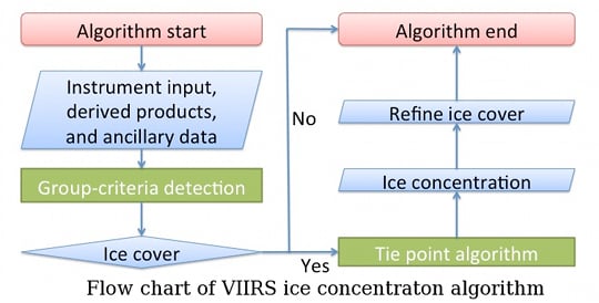
The purpose of this algorithm is to detect ice and to estimate ice concentration, i.e., the fraction of a satellite field-of-view that is covered by ice. Ice is first detected by a group-criteria method. Then ice concentration is retrieved after the visible band reflectance and ice surface temperature of pure ice are determined through a tie point algorithm. The ice cover mask is then further refined based on the retrieved ice concentration. This algorithm has a solid physical foundation and is capable of identifying ice cover mask and retrieving ice concentration in both day (sunlight) and night (dark) conditions. It runs automatically and can be applied globally. Because the surface is obscured by clouds in the visible and infrared observations, the ice cover mask and concentration can only be determined in clear-sky areas.
The accuracy of the algorithm is therefore influenced by the quality of the cloud mask. Pixels that are clear but identified as cloud do not introduce errors in the ice concentration estimates, as these pixels are excluded from the retrieval. In contrast, pixels that are cloudy but identified as clear, called “leakage”, do contribute to errors in ice concentration, as they may be labeled as ice due to their high visible reflectance and/or low temperature. The leakage rate is not known for sea ice scenes, but tests over Greenland show a leakage rate of up to 2.4% with the original VIIRS cloud detection algorithm, and as low as 0 with more recent improvements [36]. How this impacts errors in ice concentration is difficult to determine, as it depends on the proportions of ice and clouds in any given scene as well as the actually ice concentration under the pixels that were misidentified as clear. The performance of cloud mask in the polar regions in daytime is generally better than that during nighttime due to more available spectral information in daytime. This difference can lead to cloud mask discontinuity in regions that include the terminator, the boundary between the sunlit and dark portions of the earth, and hence a discontinuity in the ice cover mask and ice concentration retrievals.

2.2.1. Ice Detection

On the microphysical scale, surface albedo depends strongly on the internal structure of ice, such as brine pockets and air bubbles in the near surface layers [40]. These internal structures change with season, the state of the near surface layers, and the age of ice. Absorption and scattering in the snow and ice are determined by their internal inhomogeneities [40,41]. Sea ice and snow albedo are very high at visible wavelengths and are low at wavelengths longer than 1.4 micrometers in both Arctic and Antarctic due to stronger absorption and less backscattering in the shortwave infrared, with higher visible albedo for snow surface, as shown in Figures 9 and 10 in [41], and Figures 1 and 2 in [42]. This feature is shared by lake ice and snow-covered lake ice in both theoretical simulations and observations, as shown in Figures 2–5 in [43], and Figure 12 in [44]. Surface albedo is much lower for surfaces with melting ice and surfaces with melt ponds, with a maximum albedo in the 0.4–0.5 micrometer region and a steep decrease between 0.5 and 0.8 micrometers [41,45]. Some ice types, such as clear lake ice, grease ice, and sea ice with melt ponds, can be difficult to detect due to the very low contrast with open water [41,43].
In the absence of sunlight, we have to rely on temperature to distinguish ice from liquid water. Surface skin (radiating) temperatures over ice are lower than the melting point (273.15 K for fresh water and around 271.35 K for salt water), when the sea ice/its snow cover is not melting.
Traditionally, the Normalized Difference Snow Index (NDSI) is used to detect snow and ice. NDSI is defined as
NDSI = (R1R2)/(R1 + R2)
where R1 is the visible channel reflectance (e.g., 0.55 μm, 0.67 μm, or 0.86 μm) and R2 is the reflectance in a shortwave infrared channel (e.g., 1.6 μm or 2.2 μm). Ice is identified when NDSI is larger than some threshold. In this algorithm, 0.86 μm and 1.6 μm are used for R1 and R2, which are VIIRS bands M7 and M10. One advantage of 0.86 μm over 0.55 μm is that NDSI calculated with the 0.55 μm reflectance is high for water that is high in green pigment, causing a false snow/ice detection, while NDSI from 0.86 μm is not.
In the daytime, defined here as solar zenith angles lower than 85°, a pixel is identified as ice covered if the NDSI value is larger than 0.45, the reflectance at 0.865 μm is higher than 0.08 [46,47,48], and the surface temperature is lower than 275.0 K over both freshwater and ocean water. The reason for not using the melting temperature is that ice-covered pixels with some liquid water (leads, melt ponds, or near the ice edge) may have temperatures above the melting point. At night, defined here as solar zenith angles of 85° and higher, a pixel is identified as ice covered if the surface temperature is lower than 275.0 K over lakes, rivers (fresh water), and oceans (salt water).
Over melting ice and melt ponds, the surface albedo is low between 0.5 and 0.8 micrometers, which may cause the NDSI to misidentify melting ice and melt pond as water. When the ice is melting or very thin, the ice surface temperature is close to the melting point, which can lead to errors in the ice/no ice identification. Meanwhile, the uncertainties in the derived ice surface temperature and VIIRS reflectances can also lead to errors in the ice/no ice identification.

2.2.2. Tie Point Algorithm

The ice concentration (fraction) in any given pixel is calculated as Equation (4). Reflectances and brightness temperatures of 100% ice and 100% water are needed. These are referred to as “tie points”. However, ice characteristics can vary considerably over space and time so it is not possible to specify fixed reflectance and temperature tie points for ice. While the spectral properties of ice vary with illumination and viewing geometry, air temperature, and the physical characteristics of ice, the main reason for variability within an image is the variation in ice concentration. Therefore, the methodology is to use a search window around each pixel and build histograms of reflectance and brightness temperature in order to identify pixels that are 100% ice. The water tie point is parameterized, as described later.
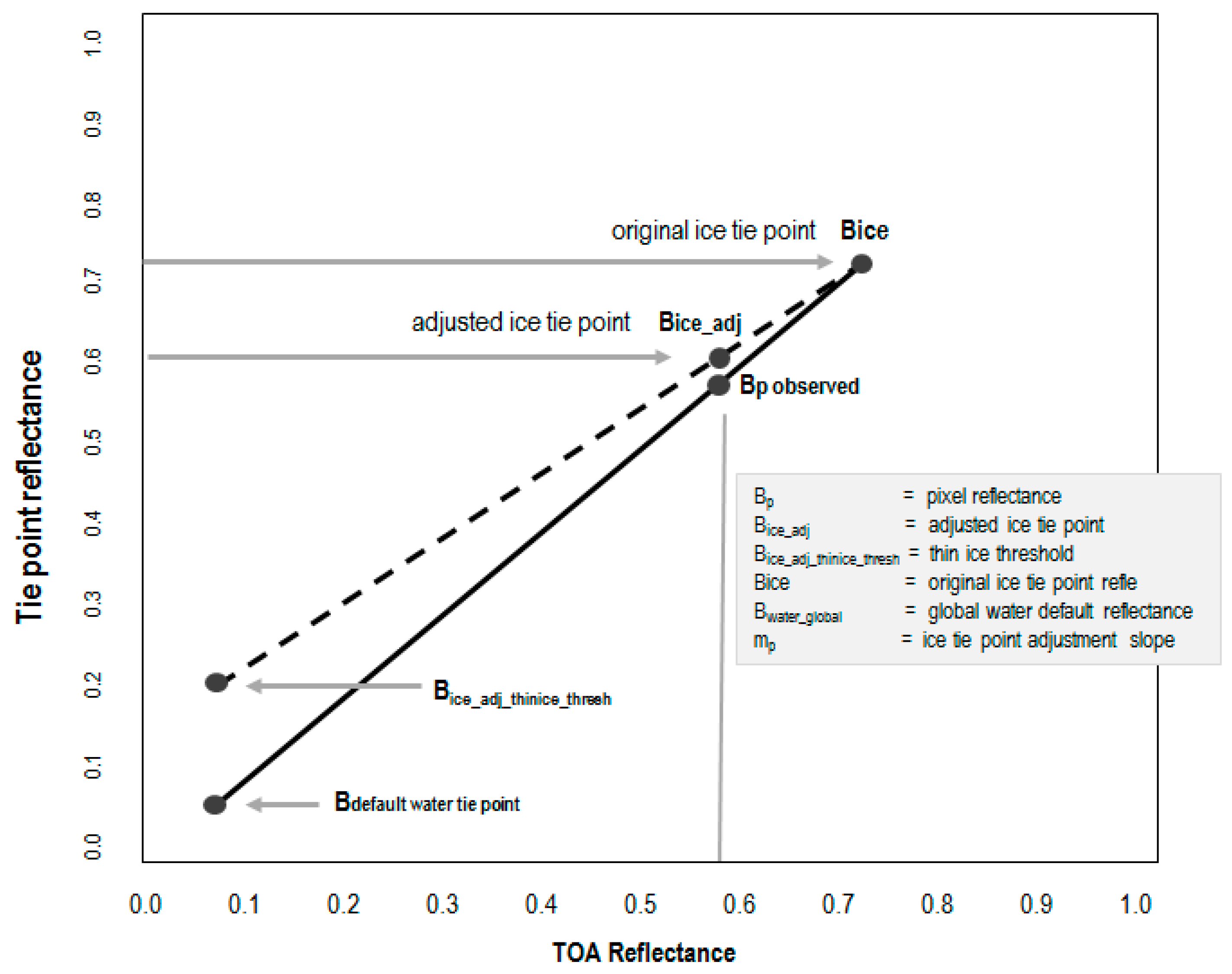
If an ice tie point can be found, then ice concentration for a pixel, Cp, at the location is calculated by
Cp = (BpBwater)/(BiceBwater)
where Bwater is the reflectance or temperature of pure water pixels, Bice is the reflectance or temperature of pure ice pixels (tie point reflectance or temperature), and Bp is the observed reflectance or temperature of the pixel. The reflectance in the visible band at 0.67 μm is used because it gives excellent spectral separation between ice (or snow on ice) and open water. In this algorithm, the visible reflectance is used during the day, and ice surface temperature is used at night.
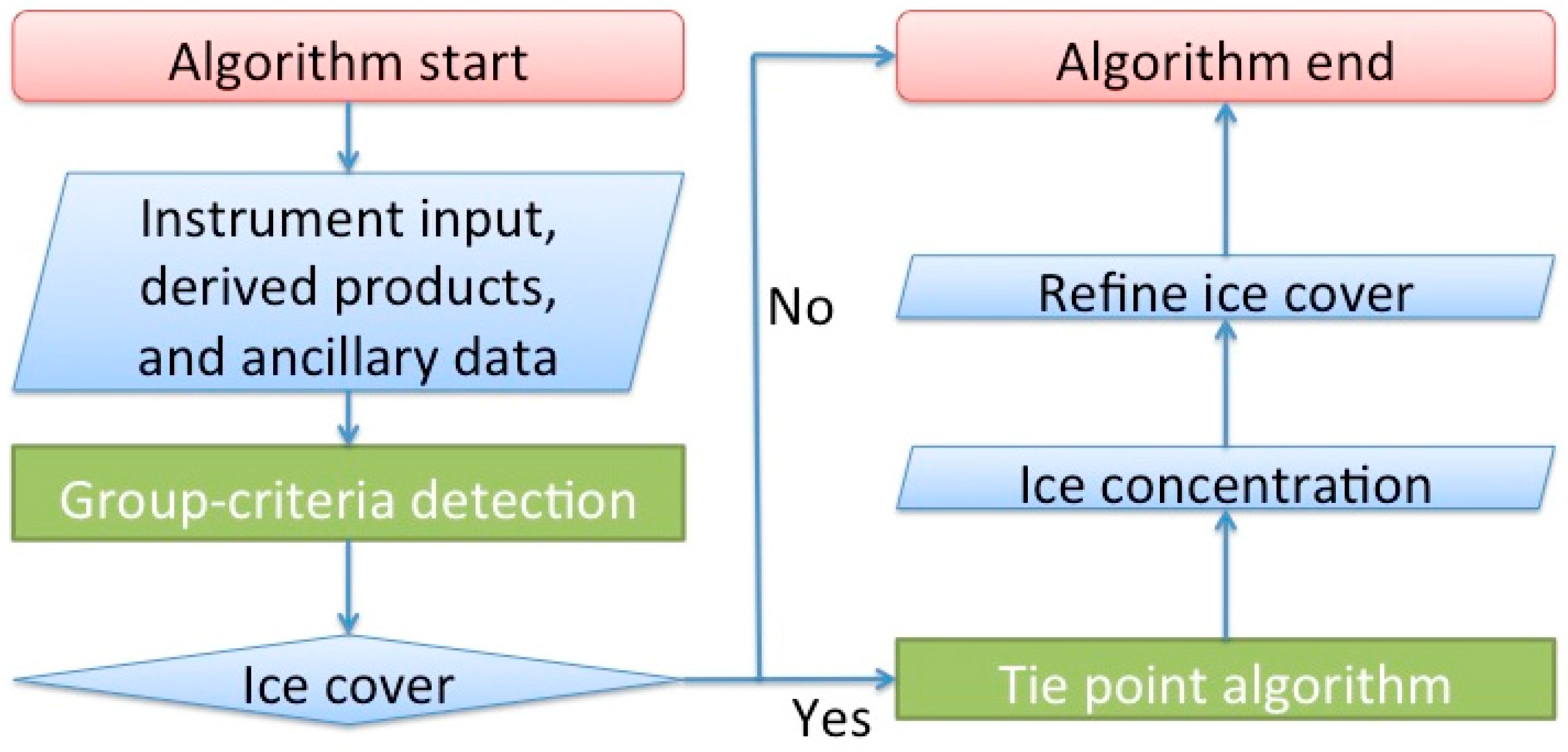
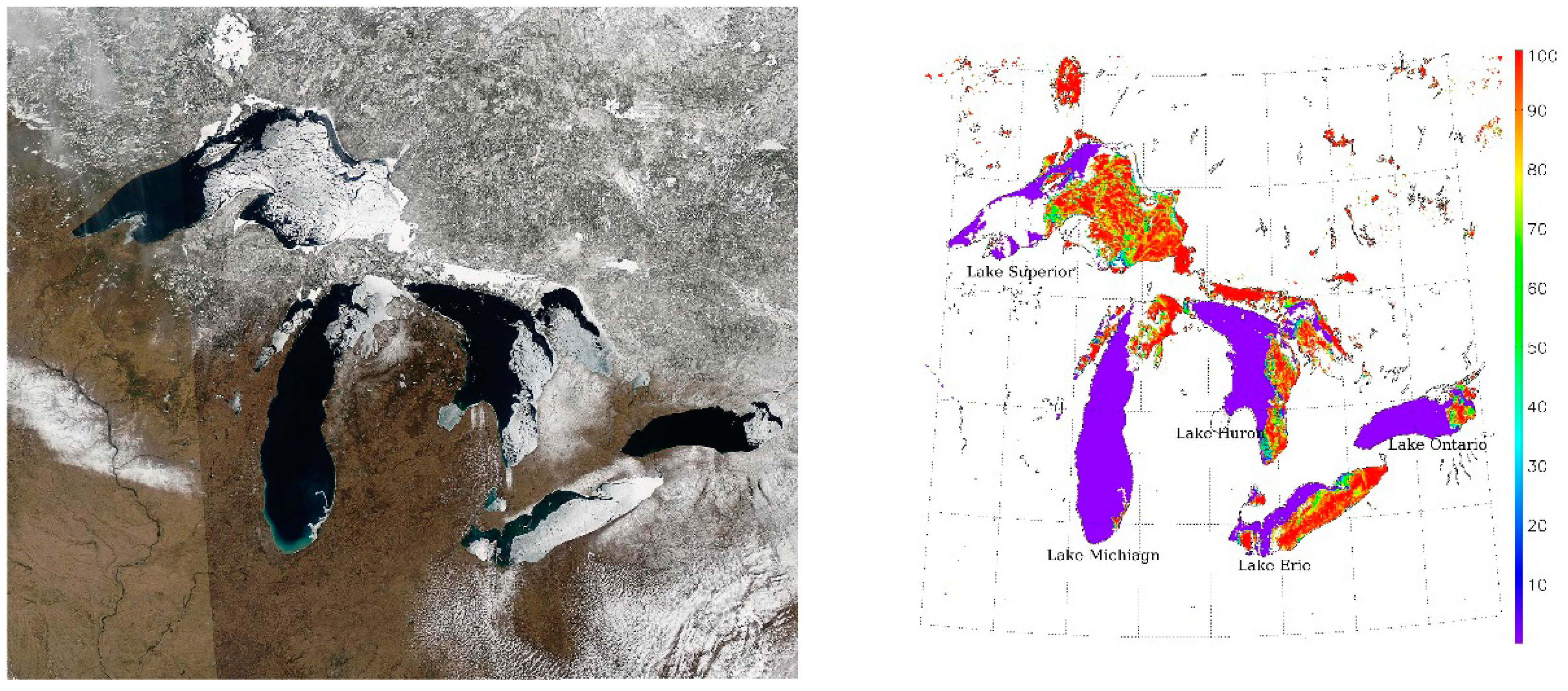
Figure 2 is an RGB (red-green-blue) image from the Landsat 8 Operational Land Imager (OLI) and VIIRS over the Kara Sea just east of Novaya Zemlya. The original spatial resolutions of the Landsat 8 OLI and VIIRS are 30 m and 750 m, which are remapped to 50 m and 1 km using the Equal-Area Scalable Earth (EASE)-Grid using the MODIS Swath-to-Grid Toolbox (MS2GT) (http://nsidc.org/data/modis/ms2gt/index.html). This scene shows pixels that are open (unfrozen) water, partially ice-covered, and fully ice-covered.
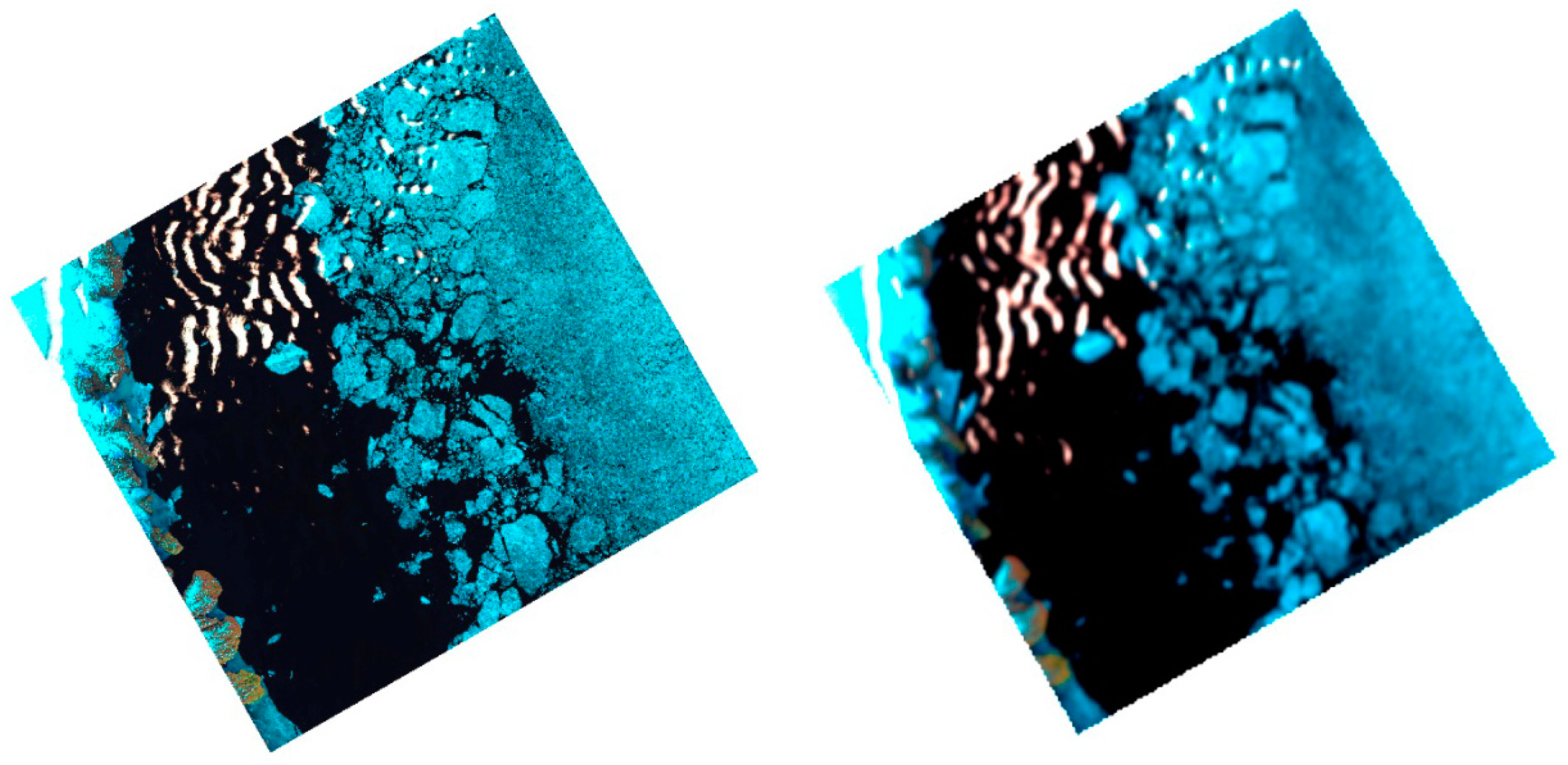
Determining the reflectance/temperature ice tie point at a location is the key to calculating the ice concentration. In a square, sliding search window with a size of N × N original VIIRS M band pixels, the ice reflectance/temperature probability density function (PDF) is calculated using all ice-covered pixels identified by the methodology in the previous section. N is set to 51 with the location of interest at the center. Retrieved tie point values are found to be insensitive to N for 31 < N < 51. This PDF is presented as a histogram; i.e., it is visualized as a relative frequency histogram. For temperature, the minimum central bin value is 215 K with a bin width of 0.5 K, and a total number of bins of 121. For reflectance, the minimum central bin value is 0.0 with bin width of 0.02; the total number of bins is also 121 to be consistent with temperature. The PDF is then smoothed using a boxcar filter with a width of 5 bins, in which a sliding integral is calculated over the original PDF. Figure 3 shows the PDF of reflectance of all the ice-covered pixels of the scene in Figure 2.
The PDF in individual search windows resembles the PDF shown in Figure 3, with narrower distributions. The ice reflectance/temperature tie point in a search window is the reflectance/temperature with the maximum probability density in the smoothed PDF, i.e., the maximum sliding integral. The ice reflectance/temperature tie point is assigned to the central pixel. It should be noted that the tie point algorithm is run only under the constraint that at least 10% of the pixels in a search window are clear-sky ice-covered pixels, and the central pixel is ice covered. The sliding search window moves 1 pixel each time to determine the tie point at each every pixel in a scene. 
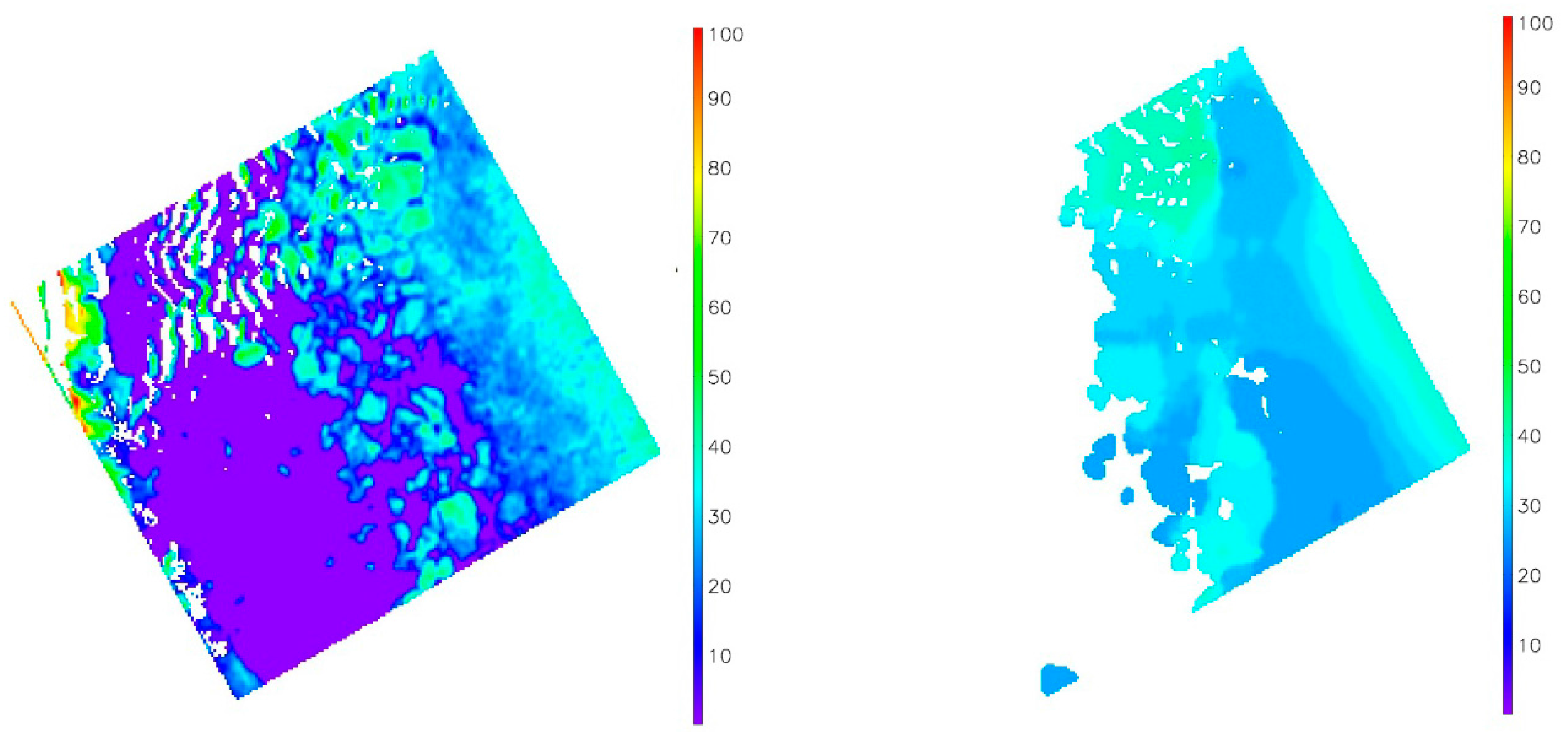
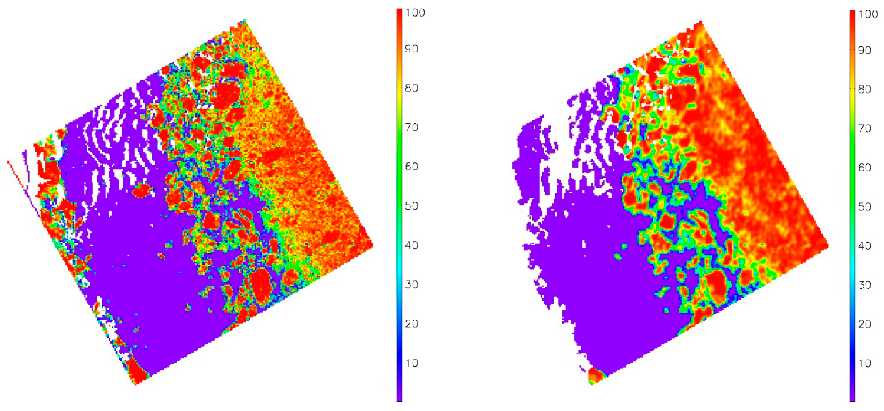
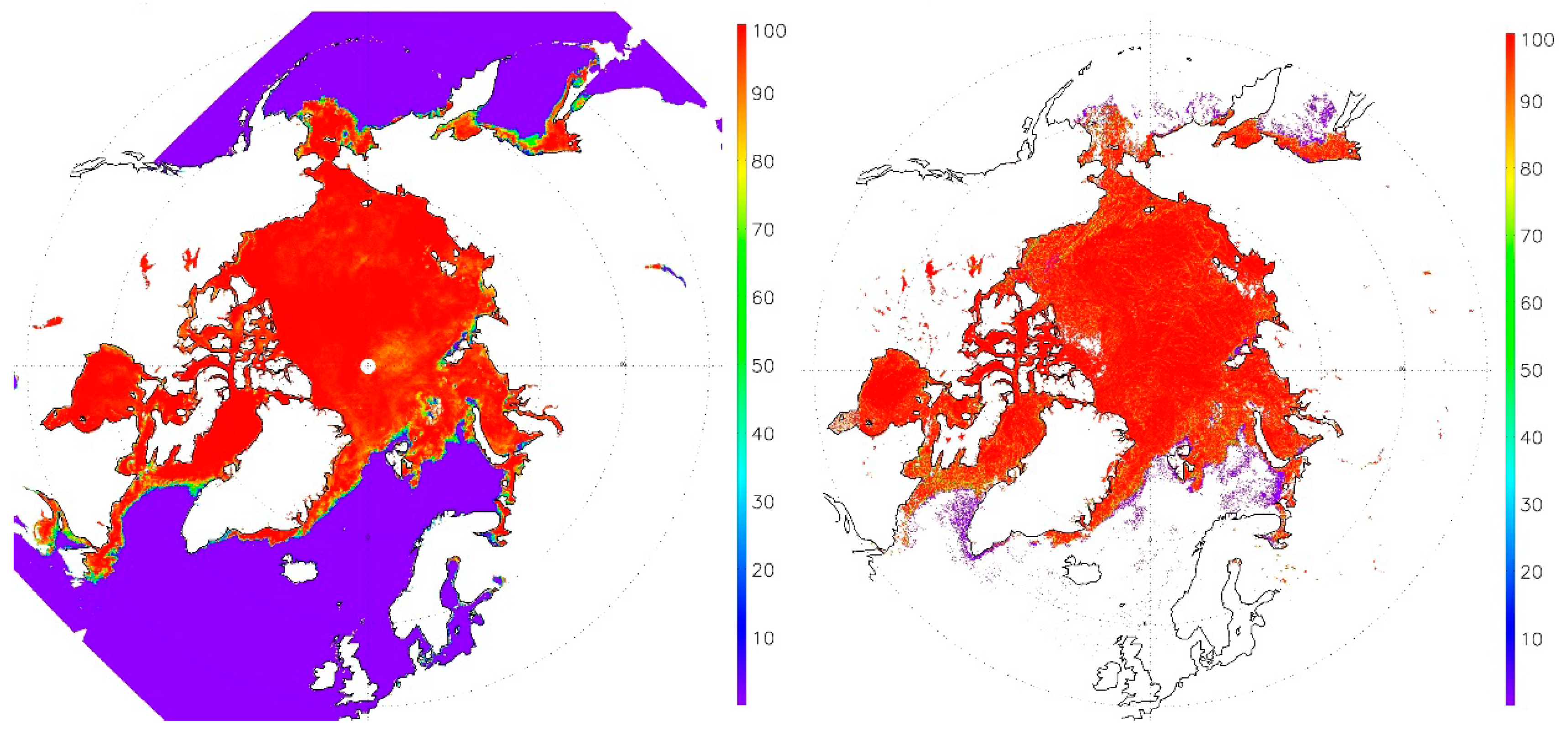
Figure 4 shows the reflectance at 0.67 μm and the derived tie points. This tie point algorithm is adapted from a similar algorithm in [49], with the assumption that 100% ice concentration occupies enough of all the available clear-sky ice-covered pixels in a search window that an ice tie point can be derived, and ice characteristics in the search window are homogeneous. When these assumptions are not satisfied, the ice concentration can have large uncertainties in regions like the marginal ice zone, and transition zones between melt pond covered and melt pond free sea ice. Due to the constraints on the available clear-sky ice-covered pixels, this tie point algorithm does not work on very small bodies of water.
While the tie point of open water could be obtained dynamically in the same way as the ice tie point, the reflectance and temperature of water within or near the ice pack does not vary as much as ice of varying thicknesses. Therefore, the water reflectance tie point is simply parameterized as a function of solar zenith angle, with a value of 0.05 for solar zenith angles less than 65°, and 0.07 for solar zenith angles greater than or equal to 65° and less than 85°. The water temperature tie point changes with the water salinity, being 273.15 K for freshwater and 271.35 K for salt water.
After the reflectance/temperature ice tie point is determined, ice concentration is calculated following Equation (4), where ice concentration is 100% if the observed reflectance is higher or the temperature is lower than the tie point, or 0% if it is lower (reflectance)/higher (temperature) than the water tie point. 
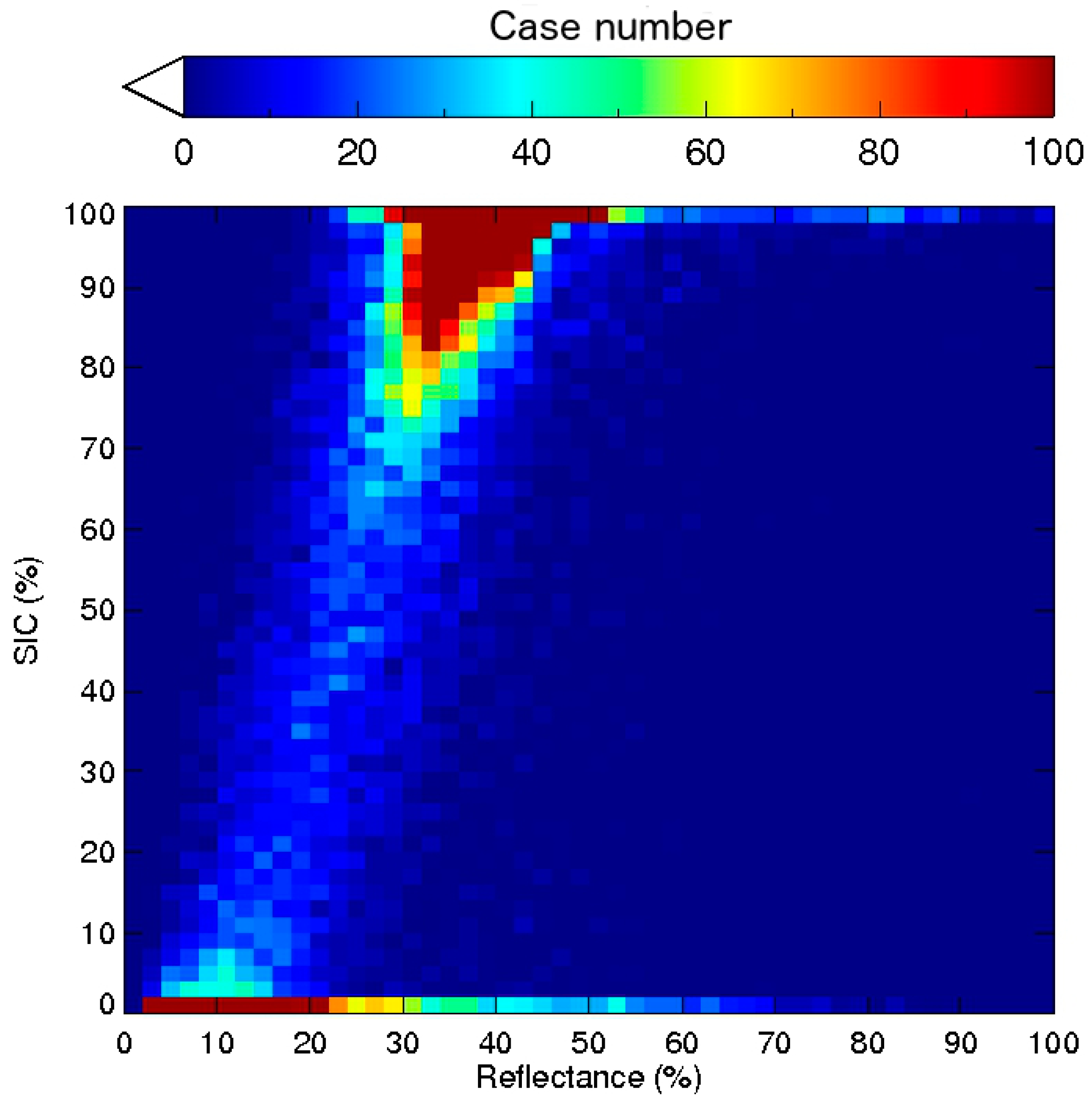
Figure 5 shows the linear relationship of the 0.64 μm reflectance and ice concentration derived from Landsat 8, which demonstrates that using Equation (4) to calculate the ice concentration is a valid approach. The large spread of 0.64 μm reflectances for ice concentrations near 0% may be due to cloud contamination, errors in the land cover data, and/or geo-location errors. Details of the Landsat 8 ice concentration calculation are given in the next section.
As the last step, the ice cover mask from the ice identification step is refined as the final ice cover mask. If the retrieved ice concentration is below 15%, the pixel is relabeled as water in the ice cover mask. This is done because the uncertainty of the estimates for low ice concentrations is 15%–20% (see next section), and to be consistent with passive microwave ice concentration products, which traditionally use the same criterion.

2.3. Validation Data

Given the lack of in situ data for validation of the VIIRS ice concentration product, the approach used here is to use very high resolution satellite data, label each pixel as either ice or open water, then calculate the percentage of ice pixels in an area the size of a VIIRS pixel. Landsat 8 is employed because it is high resolution and accessible. All Landsat 8 scenes in 2013 and 2014 containing Arctic sea ice and that are 90% or more clear sky were obtained from the U.S. Geological Survey (USGS) data server. There are a total of 181 Landsat scenes, with a scene size of 170 km by 185 km. For each scene, visible and thermal channel observations at 30 m spatial resolution are available from the OLI and the Thermal Infrared Sensor (TIRS). Only daytime images are used because of the larger calibration uncertainty associated with 12 μm band of TIRS, which is needed for surface temperature retrieval and hence nighttime ice concentration estimates. Therefore, validation with Landsat is restricted to the months of February through October.
Each pixel at the original Landsat spatial resolution is identified as either ice covered or open water using the tests detailed in Section 2.2.1. A pixel is identified as ice covered if the NDSI value, calculated from band 5 and band 6 of Landsat 8, is larger than 0.45, and if the reflectance at 0.865 μm, band 5 of Landsat 8, is higher than 0.08. The surface temperature constraint is not used. Ice concentration at the 1 km spatial resolution was calculated as the ratio of the number of 30 m Landsat ice-covered pixels to the total number of pixels in a 1 km grid cell. For each of the Landsat scenes, a corresponding VIIRS scene is found for time differences less than 1 h. This resulted in 155 matches (Figure 6). Ice concentration for all VIIRS pixels in those scenes was calculated using algorithms in Section 2.2.1 and Section 2.2.2, and then remapped to 1 km EASE-Grid.
A daily mean sea ice concentration product was also obtained from the SSMIS onboard the DMSP F17 satellite. The product has a 25 km resolution in a polar stereographic grid and is based on the NASA Team algorithm [20] from the National Snow and Ice Data Center (NSIDC). Lastly, we applied the NASA Team 2 sea ice concentration algorithm [15] to AMSR2 cases in winter, spring, and summer for an additional comparison to VIIRS ice concentration.

3. Results

The algorithm described above was applied to the 155 matched VIIRS scenes. In addition, ice concentration is produced routinely for every overpass in both poles. VIIRS ice concentration daily composites are generated by remapping individual overpasses of VIIRS ice concentration to a 1 km EASE-Grid with newer cloud free data replacing older cloud free data. An example of VIIRS ice concentration for a single S-NPP overpass over the Arctic is shown in Figure 7.

3.1. Sea Ice Concentration and Fresh Water Ice Concentration Result

Figure 8 shows the ice concentration for the scene in Figure 2, for both Landsat 8 and VIIRS. No retrievals were done from VIIRS on the left boundary of the scene because the VIIRS land mask indicates that it contains land over Novaya Zemlya, while the Landsat ice concentration does not exclude that land area. Both ice concentrations show very similar spatial distributions and values. The Landsat 8 ice concentration gives more detail, of course, with more distinct ice edges and smaller areas of open water inside the pack ice.
Figure 9 shows ice concentration from SSMIS at 25 km resolution and from a VIIRS daily composite comprised of multiple orbits at 1 km resolution on 20 February 2015. Both products show very high ice concentrations over the pack ice in the central Arctic Ocean. The passive microwave product shows relatively low concentration toward the ice edge and also near the North Pole. The ice concentration transition from high to low values is not as obvious in VIIRS product as in SSMIS, except in the southern portion of Baffin Bay. The fast ice along the Russian coast seems to have a sea ice concentration close to 100% in the VIIRS SIC map compared to the SSMIS map. This also applies to both the Kara as well as the Laptev Seas. In general, the SSMIS ice concentration product does not show much detail within the pack ice mainly due to its low spatial resolution.
In contrast, VIIRS shows much detail, particularly sea ice leads (fractures). This is illustrated in Figure 10, which shows the area from the North Pole to the Laptev and East Siberian Seas. Leads can be seen in the VIIRS product but not in the SSMIS ice concentration. Additionally, the somewhat lower concentration area near the North Pole in the SSMIS product is not seen in the VIIRS product, though there are some leads in that area. We would not expect such a large area of ice concentrations less than 90% in February around the North Pole, and do not see it in the VIIRS data. This reduced sea ice concentration may be caused by snow properties and variations in the ice–snow interface feeding back to the microwave emissivity of the sea ice [18].
Ice concentration over fresh water in lakes and rivers is also retrieved. Ice detection, the tie point algorithm, and the ice concentration calculation are done using the same approach as detailed in Section 2.2.1 and Section 2.2.2. Figure 11 (left) is a true-color image from Aqua MODIS 1 km Level 1b data on 28 March 2015, showing mostly clear conditions over the Great Lakes. The Great Lakes, between 41° and 49° latitude and −75° and −93° longitude, include five interconnecting large lakes, one small lake, four connecting channels, and the St. Lawrence Seaway, and contain the largest supply of freshwater in the world. The Aqua MODIS data is from the Level 1 and Atmosphere Archive and Distribution System (LAADS) at the Goddard Space Flight Center. The MODIS NDSI is calculated with band 2 (0.85 μm) and band 6 (1.6 μm) for Terra, and band 2 and band 7 (2.1 μm) for Aqua, as Aqua band 6 is essentially unusable. Ice surface temperature is calculated as Equation (1) based on MODIS bands 31 and 32 (11 μm and 12 μm) and viewing angles with coefficients for MODIS Terra and Aqua. A pixel is identified as ice covered if the NDSI value is larger than 0.45, and the reflectance at 0.865 μm is higher than 0.08. The surface temperature constraint is employed. The tie point method is applied to MODIS band 1 (0.64 μm), and ice concentration is calculated as Equation (4). Details of the ice cover can be seen in the eastern portions of all the lakes. Ice concentration using the algorithm presented here but with MODIS data is shown in Figure 11 (right), demonstrating the capability of detecting relatively small areas with ice coverage over the Lake Michigan and Lake Ontario, and more extensive coverage over Lake Erie, Lake Huron and Lake Superior.

3.2. Comparison of VIIRS and AMSR2 Ice Concentration

Sea ice concentration and an ice cover mask are being generated routinely and compared to similar products from other datasets, e.g., the ice concentration from SSMIS as shown in Figure 9 and from AMSR2. Sea ice concentration retrievals from VIIRS and the daily passive microwave product are collocated through remapping to a 25 km EASE-Grid with the nearest neighbor interpolation for the passive microwave data, and a weighted average for interpolation of VIIRS as detailed in MS2GT. Besides the very different spatial resolution of these two products, differences in their ice concentrations come from differences in instrument sensitivities (visible/IR versus passive microwave), instrument field-of-view, and fundamental differences in the retrieval algorithms.
Results from comparisons with AMSR2 in January through August 2015, Arctic and Antarctic, are given in Table 3. Two days from each month were examined. The bias is defined as the average difference between observations of the two products. The root-mean-square error (RMSE) is the square root of the mean squared difference of the two products. RMSE is also calculated with the bias removed, which is the square root of the average squared deviation of the errors from the mean error, or the standard deviation of the errors. For some applications, the absolute values of the bias, the RMSE, and the RMSE with the bias removed, are termed as measurement accuracy, measurement uncertainty, and measurement precision, respectively. This terminology is used in the JPSS program. Biases (accuracies) range from 0.25% to 3.2%. RMSE (precision) values are in the range 8%–20%.

3.3. Ice Concentration Validation with Landsat in Daytime

A more direct validation of VIIRS sea ice concentration is done with the use of higher resolution, rather than lower resolution, data. Bias and RMSE of ice concentration from VIIRS in comparison to Landsat 8 are calculated using the 155 collocated cases described in Section 2.3.
The ice cover mask is binary mask that can be determined from the ice concentration products following the convention that a pixel is ice covered with 15% or more ice concentration. The 155 matched VIIRS-Landsat sea ice concentration scenes pairs correspond to 2,812,734 valid, clear sky match-ups. We count the number of pixels with SIC < 15% and denote them as class “open water” and we count the pixels with SIC > 15% and denote them as class “ice”. Table 4 shows the distribution of case numbers of open water and ice from Landsat 8 and VIIRS. The overall agreement is measured as the detection accuracy, 100 × (Nice + Nwater)/N, where Nice and Nwater are the number of ice pixels and water pixels in agreement. Detection accuracy has range of 0 to 1, with 1 as the perfect score. The score for this case study is 0.97. The agreement is also expressed by the Hanssen-Kuiper Skill Score (KSS) [50], which is useful when the analyzed parameter is not normally distributed. Such is the case for ice concentration. This score expresses the hit rate relative to the false alarm rate, with range of −1 to +1, with 0 and negative as no skill, and 1 as perfect. The KSS is 0.81. However, 57,490 of total 318,843 pixels identified as water by Landsat are classified as ice by VIIRS. Compared to the low rate that pixels identified as ice by Landsat are classified as water by VIIRS, this high rate of water misclassification may result from the differences in the inputs to the VIIRS and Landsat ice concentration and differences in how the products are derived, e.g., the differences in the VIIRS and Landsat cloud mask, and tie point method is applied in VIIRS ice concentration, but not in Landsat.
Histograms of the differences between VIIRS and Landsat 8 ice concentration match-ups are shown in Figure 12 for all cases and for concentration bins of 15%–30%, 30%–50%, 50%–70%, 70%–90%, and 90%–100%. Only cases (pixels) with ice concentration from both products higher than 15% are included. For over 2 million matched pairs, the VIIRS ice concentration shows an overall bias of −0.3% and an RMSE with the bias removed of 9.5% as shown in Table 5. The majority of the ice concentration differences (biases) have absolute values less than 10.0%.
On a bin-by-bin basis the differences can be somewhat larger as shown in Table 5. For the bin with the VIIRS ice concentration between 90% and 100%, the bias is positive and small at 0.9%. The bias becomes negative for smaller VIIRS ice concentration, and becomes more negative with decreasing VIIRS ice concentration. The RMSE with bias removed values also increases with smaller VIIRS ice concentrations.
It should be noted that Landsat uses its own cloud detection, which is different from VIIRS. This difference can affect the validation results. Melting ice and melt ponds can affect the ice/no ice identification, and can lead to uncertainties in the ice concentration retrieval due to its similar temperature and reflectance with open water. As shown in Table 6, the overall bias is similar for all surface temperature subranges, and the overall RMSE is between 4% and 6% for surface temperature of 250 K or higher, but below 2% for surface temperature below 250 K. For medium ice concentration, e.g., 30%–50%, the VIIRS SIC bias and RMSE decrease with increasing surface temperature; the same applies to the bias for 50%–70%, 70%–90% and 90%–100% VIIRS SIC.

3.4. Ice Concentration Validation with Landsat Applying Nighttime Algorithm on Daytime Data

As stated in Section 2.2.2, the visible reflectance at 0.67 μm is used during the day, and ice surface temperature is used at night to calculate the VIIRS ice concentration after tie point reflectance/temperature are determined. In Section 3.3, Landsat ice concentration is used to validate the daytime algorithm for all the Landsat scenes are in daytime. To assess the nighttime algorithm, we apply it to the VIIRS scenes corresponding to the Landsat scenes, and validate the derived VIIRS ice concentration using the same Landsat ice concentration and same approach as detailed in Section 3.3, which means that the sea-ice concentration based on Landsat images is based on optical data while sea-ice concentration derived with VIIRS is solely based on thermal channel information. The results are shown in Table 7. The nighttime algorithm performance is comparable to, or better than, the daytime algorithm for surface temperatures below 260 K, especially for VIIRS ice concentrations between 30% and 90%. Both algorithms perform similarly for surface temperatures between 260 and 270 K. The daytime algorithm performs substantially better when the surface is near the melting point.

3.5. Tie Point Adjustment

The comparison of VIIRS ice concentration and Landsat 8 ice concentration demonstrates a larger absolute bias and larger RMSE for lower VIIRS ice concentrations. Similar biases were identified during prelaunch testing of the IDPS version of the VIIRS Sea Ice Concentration product [34]. Ice concentrations observed prelaunch using MODIS data as a proxy were frequently too low for lead-like features associated with thin ice or a mixture of thin ice and subpixel water. The bias towards low ice concentrations for such features is the result of the assumption that an ice tie point can be adequately defined as that of the predominant ice type within a search window.
A mechanism for reducing the bias has been implemented as a mitigation strategy. An adjusted ice tie point is computed as a function of the observed reflectance/temperature and is allowed to take on values close to the observed pixel value and to vary linearly up to the value of the ice tie point of the window (Figure 13):
mp = (BiceBice_adj_thinice_thresh)/(BiceBwater_defaultl)
Bice_adj = (mp)(BpBwater_default) + Bice_adj_thinice_thresh
where mp is the slope of the linear ice tie point adjustment for a pixel; Bp is the reflectance/temperature of the pixel; Bice is the reflectance/temperature of a pure ice pixel, i.e., the ice tie point; Bwater_default is the default tie point reflectance/temperature for water; Bice_adj is the adjusted ice tie point reflectance/temperature; and Bice_adj_thinice_thresh is the thin ice adjustment threshold reflectance/temperature.
The adjustment is applied only to regions with pixels that have temperatures below a threshold value and with ice tie point reflectance values greater than that of the minimum thin ice tie point value. The magnitude of the adjustment is tunable via the minimum thin ice reflectance thresholds (maximum temperature threshold). The adjustment scheme is applied only for the situation where few water pixels are found in a local search window. This adjustment is designed for cases in which the lead-like features are ice free or covered by thin, snow-free ice with a substantially higher temperature and/or a substantially lower reflectance.
After the adjustment methodology is implemented, the validation of S-NPP VIIRS ice concentration with Landsat 8 ice concentration reported above was updated, with results shown in Figure 14 and Table 8. The overall bias increases, with a reduction in the overall RMSE. The SIC range 90%–100% is the dominant range for all cases, and the bias and RMSE for this range increase. The bias and RMSE for the SIC ranges 15%–30%, 30%–50% and 50%–70% decrease except the RMSE for SIC range 70%–90%.
It should be noted that the tie point adjustment methodology presented here has not been implemented in the Enterprise VIIRS sea ice concentration algorithm. Its future implementation relies on a deeper understanding of the discrepancy between VIIRS ice concentration and ice concentration from Landsat and other data sources.

4. Summary and Conclusions

A new algorithm for estimating ice concentration from visible and infrared satellite images has been presented. Clear-sky sea and fresh-water ice concentration at 0.75 km resolution are produced from VIIRS visible and infrared data in both daytime and nighttime. It will be used operationally with VIIRS on the future JPSS satellites. The approach builds on previous research algorithms for the AVHRR, MODIS, and on the current operational VIIRS algorithm. It determines local ice tie points and then linearly interpolates the ice concentration for each pixel between ice and water tie points.
High-resolution Landsat 8 data were used to validate the VIIRS ice concentration. Overall, the VIIRS ice concentration has a bias of −0.3% and an RMSE with the bias removed of 9.5%. The majority of the ice concentration differences (biases) for different concentration ranges have absolute values less than 10.0%. This shows that overall the VIIRS ice concentration algorithm is performing well.
Comparisons of VIIRS and passive microwave ice concentrations reveal the strengths and weaknesses of each. Historically, passive microwave sensors have been used for ice concentration, primarily because of their all-weather capability. However, small-scale information can only be obtained from optical and infrared sensors, albeit only for clear-sky areas. Validation of VIIRS ice concentration is best performed with higher resolution optical sensors. Landsat 8 has proven to be a valuable asset for this task. SAR is a potential validation source as well, as it provides high spatial resolution data under all weather conditions. Ice concentration algorithms for SAR have been developed [51], but operational products do not yet exist. Nevertheless, such a product should be considered in the future for validating the VIIRS ice concentration.
NOAA’s operational satellite products are available from the National Centers for Environmental Information (NCEI) Comprehensive Large Array-data Stewardship System (CLASS). The Enterprise VIIRS ice concentration product is planned for operations in late 2016.

Acknowledgments

This work was supported by the JPSS Program Office and the GOES-R Program Office. We thank Richard Dworak for performing the comparison of VIIRS and AMSR2 ice concentrations. The views, opinions, and findings contained in this report are those of the author(s) and should not be construed as an official National Oceanic and Atmospheric Administration or U.S. Government position, policy, or decision.

Author Contributions

Yinghui Liu designed the research, collected most of the data, implemented most of the data analysis, and wrote the manuscript. Jeffrey Key advised the whole study, and made significant revisions of the manuscript. Robert Mahoney contributed the tie point adjustment and was involved in product validation. All the authors contributed to the revisions of the manuscript.

Conflicts of Interest

The authors declare no conflict of interest.

References

  1. Serreze, M.C.; Stroeve, J. Arctic sea ice trends, variability and implications for seasonal ice forecasting. Philos. Trans. R. Soc. A 2015, 373. [Google Scholar] [CrossRef] [PubMed]
  2. Stroeve, J.C.; Serreze, M.C.; Holland, M.M.; Kay, J.E.; Malanik, J.; Barrett, A.P. The Arctic’s rapidly shrinking sea ice cover: A research synthesis. Clim. Chang. 2012, 110, 1005–1027. [Google Scholar] [CrossRef]
  3. Maslanik, J.; Stroeve, J.; Fowler, C.; Emery, W. Distribution and trends in Arctic sea ice age through spring 2011. Geophys. Res. Lett. 2011, 38. [Google Scholar] [CrossRef]
  4. Kwok, R.; Cunningham, G.F. Variability of Arctic sea ice thickness and volume from Cryosat-2. Philos. Trans. R. Soc. Lond. A Math. Phys. Eng. Sci. 2015, 373, 20140157. [Google Scholar] [CrossRef] [PubMed]
  5. Parkinson, C.L.; Cavalieri, D.J. Antarctic sea ice variability and trends, 1979–2010. Cryosphere 2012, 6, 871–880. [Google Scholar] [CrossRef]
  6. Liu, Y.; Key, J.; Wang, X. Influence of changes in sea ice concentration and cloud cover on recent arctic surface temperature trends. Geophys. Res. Lett. 2009, 36. [Google Scholar] [CrossRef]
  7. Schweiger, A.J.; Lindsay, R.W.; Vavrus, S.; Francis, J.A. Relationships between Arctic sea ice and clouds during autumn. J. Clim. 2008, 21, 4799–4810. [Google Scholar] [CrossRef]
  8. Liu, Y.; Key, J.; Liu, Z.; Wang, X.; Vavrus, S. A cloudier arctic expected with diminishing sea ice. Geophys. Res. Lett. 2012, 39, L05705. [Google Scholar] [CrossRef]
  9. Taylor, P.C.; Kato, S.; Xu, K.-M.; Cai, M.C.J.D. Covariance between Arctic sea ice and clouds within atmospheric state regimes at the satellite footprint level. J. Geophys. Res. Atmos. 2015, 120, 12656–12678. [Google Scholar] [CrossRef]
  10. Cohen, J.; Screen, J.A.; Furtado, J.C.; Barlow, M.; Whittleston, D.; Coumou, D.; Francis, J.; Dethloff, K.; Entekhabi, D.; Overland, J. Recent arctic amplification and extreme mid-latitude weather. Nat. Geosci. 2014, 7, 627–637. [Google Scholar] [CrossRef] [Green Version]
  11. Wu, B.; Handorf, D.; Dethloff, K.; Rinke, A.; Hu, A. Winter weather patterns over northern Eurasia and Arctic sea ice loss. Mon. Weather Rev. 2013, 141, 3786–3800. [Google Scholar] [CrossRef]
  12. Wu, B.; Su, J.; D’Arrigo, R. Patterns of Asian winter climate variability and links to Arctic sea ice. J. Clim. 2015, 28, 6841–6858. [Google Scholar] [CrossRef]
  13. Francis, J.A.; White, D.M.; Cassano, J.J.; Gutowski, W.J., Jr.; Hinzman, L.D.; Holland, M.M.; Steele, M.A.; Voeroesmarty, C.J. An Arctic hydrologic system in transition: Feedbacks and impacts on terrestrial, marine, and human life. J. Geophys. Res. Biogeosci. 2009, 114. [Google Scholar] [CrossRef]
  14. Cavalieri, D.J.; Gloersen, P.; Campbell, W.J. Determination of sea ice parameters with the NIMBUS-7 SMMR. J. Geophys. Res. Atmos. 1984, 89, 5355–5369. [Google Scholar] [CrossRef]
  15. Markus, T.; Cavalieri, D.J. An enhancement of the NASA team sea ice algorithm. IEEE Trans. Geosci. Remote Sens. 2000, 38, 1387–1398. [Google Scholar] [CrossRef]
  16. Comiso, J.C. Characteristics of arctic winter sea ice from satellite multispectral microwave observations. J. Geophys. Res. Oceans 1986, 91, 975–994. [Google Scholar] [CrossRef]
  17. Kaleschke, L.; Lüpkes, C.; Vihma, T.; Haarpaintner, J.; Bochert, A.; Hartmann, J.; Heygster, G. SSM/I sea ice remote sensing for mesoscale ocean-atmosphere interaction analysis. Can. J. Remote Sens. 2001, 27, 526–537. [Google Scholar] [CrossRef]
  18. Ivanova, N.; Pedersen, L.T.; Tonboe, R.T.; Kern, S.; Heygster, G.; Lavergne, T.; Sørensen, A.; Saldo, R.; Dybkjær, G.; Brucker, L. Inter-comparison and evaluation of sea ice algorithms: Towards further identification of challenges and optimal approach using passive microwave observations. Cryosphere 2015, 9, 1797–1817. [Google Scholar] [CrossRef] [Green Version]
  19. Ivanova, N.; Johannessen, O.M.; Pedersen, L.T.; Tonboe, R.T. Retrieval of Arctic sea ice parameters by satellite passive microwave sensors: A comparison of eleven sea ice concentration algorithms. IEEE Trans. Geosci. Remote Sens. 2014, 52, 7233–7246. [Google Scholar] [CrossRef]
  20. Cavalieri, D.J.; Parkinson, C.L.; Gloersen, P.; Comiso, J.C.; Zwally, H.J. Deriving long-term time series of sea ice cover from satellite passive-microwave multisensor data sets. J. Geophys. Res. Oceans 1999, 104, 15803–15814. [Google Scholar] [CrossRef]
  21. Cavalieri, D.J.; Parkinson, C.L.; DiGirolamo, N.; Ivanoff, A. Intersensor calibration between F13 SSM/I and F17 SSMIS for global sea ice data records. IEEE Geosci. Remote Sens. Lett. 2012, 9, 233–236. [Google Scholar] [CrossRef]
  22. Beitsch, A.; Kaleschke, L.; Kern, S. Investigating high-resolution AMSR2 sea ice concentrations during the February 2013 fracture event in the Beaufort Sea. Remote Sens. 2014, 6, 3841–3856. [Google Scholar] [CrossRef]
  23. Comiso, J.C.; Cavalieri, D.J.; Markus, T. Sea ice concentration, ice temperature, and snow depth using AMSR-E data. IEEE Trans. Geosci. Remote Sens. 2003, 41, 243–252. [Google Scholar] [CrossRef]
  24. Dierking, W. Sea ice monitoring by synthetic aperture radar. Oceanography 2013, 26, 100–111. [Google Scholar] [CrossRef]
  25. Fily, M.; Rothrock, D.A. Extracting sea ice data from satellite SAR imagery. IEEE Trans. Geosci. Remote Sens. 1986, GE-24, 849–854. [Google Scholar] [CrossRef]
  26. Massom, R.; Comiso, J.C. The classification of Arctic sea ice types and the determination of surface temperature using advanced very high resolution radiometer data. J. Geophys. Res. Oceans 1994, 99, 5201–5218. [Google Scholar] [CrossRef]
  27. Lindsay, R.W.; Rothrock, D.A. Arctic sea ice leads from Advanced Very High Resolution Radiometer images. J. Geophys. Res. 1995, 100, 4533–4544. [Google Scholar] [CrossRef]
  28. Comiso, J.C.; Steffen, K. Studies of Antarctic sea ice concentrations from satellite data and their applications. J. Geophys. Res. 2001, 106, 31361–31385. [Google Scholar] [CrossRef]
  29. Drue, C.; Heinemann, G. High-resolution maps of the sea-ice concentration from MODIS satellite data. Geophys. Res. Lett. 2004, 31. [Google Scholar] [CrossRef]
  30. Drue, C.; Heinemann, G. Accuracy assessment of sea-ice concentrations from MODIS using in-situ measurements. Remote Sens. Environ. 2005, 95, 139–149. [Google Scholar] [CrossRef]
  31. Baker, N. Joint Polar Satellite System (JPSS) VIIRS Sea Ice Characterization Algorithm Theoretical Basis Document (ATBD). 2011. Available online: http://npp.gsfc.nasa.gov/sciencedocs/2015-06/474-00047_VIIRS_Sea_Ice_ATBD_Rev-20110422.pdf (accessed on 22 April 2011). [Google Scholar]
  32. Rösel, A.; Kaleschke, L.; Birnbaum, G. Melt ponds on Arctic sea ice determined from MODIS satellite data using an artificial neural network. Cryosphere 2012, 6, 431–446. [Google Scholar] [CrossRef] [Green Version]
  33. Cao, C.; Xiong, J.; Blonski, S.; Quanhua, L.; Uprety, S.; Xi, S.; Yan, B.; Fuzhong, W. Suomi NPP VIIRS data record verification, validation, and long-term performance monitoring. J. Geophys. Res. Atmos. 2013, 118, 11664–11678. [Google Scholar] [CrossRef]
  34. Hutchison, K.D.; Cracknell, A.P. Visible Infrared Imager Radiometer Suite, a New Operational Cloud Imager; CRC Press, Taylor and Francis Group: Boca Raton, FL, USA, 2006. [Google Scholar]
  35. Wolfe, R.E.; Lin, G.; Nishihama, M.; Tewari, K.P.; Tilton, J.C.; Isaacman, A.R. Suomi NPP VIIRS prelaunch and on-orbit geometric calibration and characterization. J. Geophys. Res. Atmos. 2013, 118, 11508–11521. [Google Scholar] [CrossRef]
  36. Hutchison, K.D.; Roskovensky, J.K.; Jackson, J.M.; Heidinger, A.K.; Kopp, T.J.; Pavolonis, M.J.; Frey, R. Automated cloud detection and classification of data collected by the Visible Infrared Imager Radiometer Suite (VIIRS). Int. J. Remote Sens. 2005, 26, 4681–4706. [Google Scholar] [CrossRef]
  37. Heidinger, A.K.; Evan, A.T.; Foster, M.J.; Walther, A. A naive Bayesian cloud-detection scheme derived from CALIPSO and applied within PATMOS-x. J. Appl. Meteorol. Climatol. 2012, 51, 1129–1144. [Google Scholar] [CrossRef]
  38. Key, J.; Haefliger, M. Arctic ice surface-temperature retrieval from AVHRR thermal channels. J. Geophys. Res. Atmos. 1992, 97, 5885–5893. [Google Scholar] [CrossRef]
  39. Key, J.R.; Collins, J.B.; Fowler, C.; Stone, R.S. High-latitude surface temperature estimates from thermal satellite data. Remote Sens. Environ. 1997, 61, 302–309. [Google Scholar] [CrossRef]
  40. Grenfell, T.C.; Maykut, G.A. The optical properties of ice and snow in the Arctic basin. J. Glaciol. 1977, 18, 445–463. [Google Scholar]
  41. Perovich, D.K. The Optical Properties of Sea Ice; CRREL Monogr, No. 96-1; U.S. Army Cold Regions Research and Engineering Laboratory: Hanover, NH, USA, 1996; p. 25. [Google Scholar]
  42. Brandt, R.E.; Warren, S.G.; Worby, A.P.; Grenfell, T.C. Surface albedo of the Antarctic Sea ice zone. J. Clim. 2005, 18, 3606–3622. [Google Scholar] [CrossRef]
  43. Bolsenga, S.J. Spectral reflectances of snow and fresh-water ice from 340 through 1100 nm. J. Glaciol. 1983, 29, 296–305. [Google Scholar]
  44. Mullen, P.C.; Warren, S.G. Theory of the optical properties of lake ice. J. Geophys. Res. Atmos. 1988, 93, 8403–8414. [Google Scholar] [CrossRef]
  45. Tschudi, M.A.; Maslanik, J.A.; Perovich, D.K. Derivation of melt pond coverage on Arctic sea ice using MODIS observations. Remote Sens. Environ. 2008, 112, 2605–2614. [Google Scholar] [CrossRef]
  46. Hall, D.K.; Riggs, G.A.; Salomonson, V.V. Algorithm Theoretical Basis Document for the MODIS Snow and Sea Ice Mapping Algorithms. 2001. Available online: https://eospso.gsfc.nasa.gov/sites/default/files/atbd/atbd_mod10.pdf (accessed on 1 September 2001). [Google Scholar]
  47. Hall, D.K.; Riggs, G.A.; Salomonson, V.V. MODIS Sea Ice Products User Guide to Collection 6. 2015. Available online: http://nsidc.org/data/docs/daac/modis/pdf/modis-sea-ice-user-guide-C6.pdf (accessed on 17 March 2015).
  48. Riggs, G.A.; Hall, D.K.; Ackerman, S.A. Sea ice extent and classification mapping with the Moderate Resolution Imaging Spectroradiometer Airborne Simulator. Remote Sens. Environ. 1999, 68, 152–163. [Google Scholar] [CrossRef]
  49. Appel, I.; Jensen, K.A. Fresh Water Ice Visible/Infrared Imager/Radiometer Suite Algorithm Theoretical Basis Document; Version 5; SBRS Document SBRS-Y2404; 2002. Available online: https://www.ntis.gov/Search/Home/titleDetail/?abbr=PB2005102024 (accessed on 19 June 2016).
  50. Hanssen, A.W.; Kuipers, W.J.A. On the Relationship between the Frequency of Rain and Various Meteorological Parameters; Mededelingen en verhandelingen; Staatsdrukkerij- en Uitgeverijbedrijf: s-Gravenhage, The Netherlands, 1965; Volume 81, pp. 2–15. [Google Scholar]
  51. Karvonen, J. A sea ice concentration estimation algorithm utilizing radiometer and SAR data. Cryosphere 2014, 8, 1639–1650. [Google Scholar] [CrossRef]
Figure 1. High level processing flow diagram of the ice cover mask and concentration algorithm.
Remotesensing 08 00523 g001
Figure 2. (left) Natural-color RGB image combination of Landsat 8 Operational Land Imager (OLI) band 5 (1.6 μm, red component), band 4 (0.86 μm, green component) and band 3 (0.64 μm, blue component) resampled to 50 m resolution; and (right) VIIRS M-band natural-color RGB image combination of band M10 (1.6 μm, red component), band M7 (0.86 μm, green component), and band M5 (0.67 μm, blue component) resampled to 1 km resolution. The images cover the Kara Sea east of Novaya Zemlya at 7:59 a.m. UTC on 25 June 2013. Sea ice and snow-covered sea ice are cyan; water is black; clouds are white.
Remotesensing 08 00523 g002
Figure 3. Probability density distribution of 0.67 μm reflectance for the ice covered pixels shown in Figure 2.
Remotesensing 08 00523 g003
Figure 4. (left) Reflectance at 0.67 μm from S-NPP VIIRS; and (right) derived tie points at 0.67 μm.
Remotesensing 08 00523 g004
Figure 5. Reflectance and sea ice concentration (SIC) relative frequency distribution at 0.64 μm for Landsat ice cover in Figure 2.
Remotesensing 08 00523 g005
Figure 6. (left) spatial distribution of the center point of 155 Landsat 8 scenes; and (right) the monthly distribution of scenes.
Remotesensing 08 00523 g006
Figure 7. Ice concentration over the Arctic Ocean from the VIIRS overpass 8:43 p.m. to 9:03 p.m. UTC on 20 February 2015. The cloud-covered areas are white.
Remotesensing 08 00523 g007
Figure 8. (left) Sea ice concentration derived from the Landsat image in Figure 2; and (right) the calculated sea ice concentration using the Suomi NPP VIIRS data in Figure 2. White areas denote pixels flagged out as either land or cloudy.
Remotesensing 08 00523 g008
Figure 9. Ice concentration from SSMIS (left); and a daily ice concentration composite from VIIRS (right) over the Arctic on 20 February 2015. White areas in the SSMIS image denote pixels flagged as either land or the area around the pole that is not covered by the instrument. White areas in the VIIRS data denote pixels flagged as land, ice-free ocean, or cloud.
Remotesensing 08 00523 g009
Figure 10. Ice concentration from SSMIS (left); and from VIIRS daily composite (right) over portion of the Arctic (longitude: 90–180, latitude: 70–90) on 20 February 2015. The North Pole is in the lower left corner. White areas in the SSMIS denote pixels flagged as either land or the area around the pole that is not covered by the instrument. White areas in the VIIRS data denote pixels flagged as either land or cloudy.
Remotesensing 08 00523 g010
Figure 11. Aqua MODIS true-color image at 6:20 p.m. UTC on 28 March 2015 (left); and the corresponding ice concentration (right).
Remotesensing 08 00523 g011
Figure 12. Comparison of VIIRS minus Landsat ice concentrations for different concentration ranges/bins. Note that for “All” and “90–100” plots the vertical axis range is different than for other sea ice concentration ranges.
Remotesensing 08 00523 g012
Figure 13. The ice tie point adjustment scheme.
Remotesensing 08 00523 g013
Figure 14. Comparison of VIIRS and Landsat ice concentrations for different concentration ranges/bins when a tie point adjustment scheme is employed.
Remotesensing 08 00523 g014
Table 1. Summary of the Visible Infrared Imaging Radiometer Suite (VIIRS) Band Numbers and Wavelengths.
Band NumberBand Wavelength (μm)Horizontal Sample Interval (km)
NadirEnd of Scan
M50.6720.75 × 0.751.60 × 1.58
M70.8620.75 × 0.751.60 × 1.58
M101.6020.75 × 0.751.60 × 1.58
M1510.7290.75 × 0.751.60 × 1.58
M1611.8450.75 × 0.751.60 × 1.58
Table 2. Values of coefficients in Equation (1) for Suomi National Polar Orbiting Partnership (S-NPP) VIIRS.
Temperature Rangeabcd
Arctic<240 K7.5609931.0313441.2481510.406514
240–260 K8.9186371.0366580.5142562.111948
>260 K6.8728861.0282881.0197832.340682
Antarctic<240 K2.3988631.0107770.2253800.457090
240–260 K9.6889471.0402700.4632952.862228
>260 K9.0169851.0369050.3301302.595204
Table 3. Statistics for a comparison of VIIRS and AMSR2 ice concentration for cases in 2015.
DateArcticAntarctic
AccuracyPrecisionCasesAccuracyPrecisionCases
30 January1.618.76123,7470.5021.4522,776
31 January1.629.10124,5141.5322.0319,556
27 February2.059.91122,3761.0420.1920,101
28 February2.039.35120,3430.2120.8822,256
30 March2.4510.01122,1081.5214.9048,343
31 March2.129.39118,8412.4815.2443,737
30 April3.0211.9888,9591.8512.6479,228
31 April3.0111.8779,7562.2412.6282,094
30 May3.2011.4665,4182.1913.0399,093
31 May3.2211.9270,9901.8012.97104,142
30 June2.1914.0556,8641.5511.08121,964
31 June1.8914.4155,5801.5611.78123,805
30 July1.8918.3335,5772.4312.62142,350
31 July2.5318.2038,0692.5812.34138,524
30 August0.2518.4828,7272.7911.87133,027
31 August0.6117.1927,3152.9512.71142,208
Table 4. VIIRS/Landsat ice and water classification results.
Landsat IceLandsat Water
VIIRS ice2,479,81457,490
VIIRS water14,077261,353
Table 5. Bias and RMSE with bias removed (precision) for comparisons of VIIRS minus Landsat ice concentrations for different concentration ranges/bins.
OverallVIIRS SIC 15%–30%VIIRS SIC 30%–50%VIIRS SIC 50%–70%VIIRS SIC 70%–90%VIIRS SIC 90%–100%
Case number2,479,814778427,73266,977262,7612,114,560
Bias (%)−0.3−15.6−16.9−11.7−4.80.9
RMSE (%)9.520.426.022.614.46.4
Table 6. Bias and RMSE with bias removed (precision) for comparison of VIIRS minus Landsat ice concentrations for different concentration ranges/bins for different surface temperature ranges with match-up pairs more than 1000.
OverallVIIRS SIC 15%−30%VIIRS SIC 30%–50%VIIRS SIC 50%–70%VIIRS SIC 70%–90%VIIRS SIC 90%–100%
Surface TemperatureBias/RMSE (%)Bias/RMSE (%)Bias/RMSE (%)Bias/RMSE (%)Bias/RMSE (%)Bias/RMSE (%)
<240 K0.0/0.9
240–250 K−0.1/1.5 −8.2/16.9−0.3/3.4
250–260 K−0.2/5.4 −32.4/27.8−21.2/21.5−9.7/14.50.5/7.1
260–270 K−0.3/4.8−22.9/24.7−24.0/26.8−15.2/22.5−5.4/14.30.6/6.3
>270 K0.3/5.9−12.5/17.3−9.4/22.2−5.4/21.1−2.2/13.71.6/6.3
Table 7. VIIRS minus Landsat ice concentrations bias and RMSE with bias removed (precision) for cases where the nighttime ice concentration algorithm was applied to daytime data, over different concentration ranges/bins for different surface temperature ranges with match up pairs more than 1000.
OverallVIIRS SIC 15%–30%VIIRS SIC 30%–50%VIIRS SIC 50%–70%VIIRS SIC 70%–90%VIIRS SIC 90%–100%
Surface TemperatureBias/RMSE (%)Bias/RMSE (%)Bias/RMSE (%)Bias/RMSE (%)Bias/RMSE (%)Bias/RMSE (%)
<240 K0.0/0.7
240–250 K−0.2/1.8 −9.1/13.2−0.9/3.7
250–260 K−0.4/6.3 −13.4/24.2−16.4/22.8−8.9/14.00.0/7.2
260–270 K−0.2/6.4−27.5/29.3−16.7/26.4−12.1/23.0−6.1/15.01.4/8.7
>270 K−3.0/12.6−71.4/15.0−54.7/14.4−35.6/13.0−16.4/12.12.6/12.1
Table 8. Bias and RMSE with bias removed (precision) for comparisons of VIIRS minus Landsat ice concentrations for different concentration ranges/bins after tie point adjustment.
OverallVIIRS SIC 15%–30%VIIRS SIC 30%–50%VIIRS SIC 50%–70%VIIRS SIC 70%–90%VIIRS SIC 90%–100%
Case number2,480,093605516,55934,428168,0092,255,042
Bias (%)1.4−12.6−9.1−4.50.31.6
RMSE (%)8.917.422.421.717.27.2

