Article

Downscaling of MODIS One Kilometer Evapotranspiration Using Landsat-8 Data and Machine Learning Approaches

1
Beijing Laboratory of Water Security, Base of the State Key Laboratory of Urban Environment Process & Digital Modeling, Capital Normal University, Beijing 100089, China
2
School of Urban and Environmental Engineering, Ulsan National Institute of Science and Technology (UNIST), Ulsan 44919, South Korea
*
Author to whom correspondence should be addressed.
Remote Sens. 2016, 8(3), 215; https://doi.org/10.3390/rs8030215
Submission received: 12 December 2015 / Revised: 22 February 2016 / Accepted: 1 March 2016 / Published: 8 March 2016

Abstract

:
This study presented a MODIS 8-day 1 km evapotranspiration (ET) downscaling method based on Landsat 8 data (30 m) and machine learning approaches. Eleven indicators including albedo, land surface temperature (LST), and vegetation indices (VIs) derived from Landsat 8 data were first upscaled to 1 km resolution. Machine learning algorithms including Support Vector Regression (SVR), Cubist, and Random Forest (RF) were used to model the relationship between the Landsat indicators and MODIS 8-day 1 km ET. The models were then used to predict 30 m ET based on Landsat 8 indicators. A total of thirty-two pairs of Landsat 8 images/MODIS ET data were evaluated at four study sites including two in United States and two in South Korea. Among the three models, RF produced the lowest error, with relative Root Mean Square Error (rRMSE) less than 20%. Vegetation greenness related indicators such as Normalized Difference Vegetation Index (NDVI), Enhanced Vegetation Index (EVI), Soil Adjusted Vegetation Index (SAVI), and vegetation moisture related indicators such as Normalized Difference Infrared Index—Landsat 8 OLI band 7 (NDIIb7) and Normalized Difference Water Index (NDWI) were the five most important features used in RF model. Temperature-based indicators were less important than vegetation greenness and moisture-related indicators because LST could have considerable variation during each 8-day period. The predicted Landsat downscaled ET had good overall agreement with MODIS ET (average rRMSE = 22%) and showed a similar temporal trend as MODIS ET. Compared to the MODIS ET product, the downscaled product demonstrated more spatial details, and had better agreement with in situ ET observations (R2 = 0.56). However, we found that the accuracy of MODIS ET was the main control factor of the accuracy of the downscaled product. Improved coarse-resolution ET estimation would result in better finer-resolution estimation. This study proved the potential of using machine learning approaches for ET downscaling considering their effectiveness and ease of implementation. Future research includes development of the spatial-temporal fusion models of Landsat data and MODIS ET in order to increase temporal resolution of downscaled ET.

Graphical Abstract

1. Introduction

Land surface evapotranspiration (ET) is an important hydrological process that controls water and energy transfer between soil, vegetation, and atmosphere. Quantification of ET is extensively needed in many agricultural, forest, and climatic applications. At local to regional scales, information on the spatial and temporal variations of ET is vital for drought monitoring, ecosystem health assessment, water requirement evaluation, and agricultural water allocation and management [1]. At regional to global scales, quantifying ET is essential for mesoscale and global circulation modeling as it affects water and energy cycles between land, ocean, and atmosphere [2]. As satellite remote sensing techniques can provide viable approaches for land surface process monitoring over large areas, various approaches have been developed for ET estimation from moderate to low resolutions based on remotely sensed data during the last few decades. These approaches generally include empirical/statistical methods that link land surface temperature (LST) and/or vegetation indices (VI) with in situ ET measurements, and more physically-based models including surface energy balance (SEB) models such as Surface Energy Balance Algorithm for Land (SEBAL) [3,4], Mapping EvapoTRanspiration with Internalized Calibration (METRIC) [5], Atmosphere-Land Exchange Inverse (ALEXI) model [6], and Surface Energy Balance System (SEBS) models [7], and Penman–Monteith models [8].
The Moderate Resolution Imaging Spectroradiometer (MODIS) global evapotranspiration products (MOD16) are the first 1 km land surface ET dataset for the 109,030,000 km2 global vegetated land surface at 8-day, monthly, and annual intervals [9]. The products were developed using a Penman-Monteith approach driven by MODIS derived surface albedo, land cover, Leaf Area Index (LAI), the Fraction of absorbed Photosynthetically Active Radiation (FPAR), and daily surface meteorological parameters [9,10]. Various studies have evaluated the products over different regions and shown that they agree well with the other satellite or model-based ET datasets, such as the EUropean Organisation for the Exploitation of METeorological SATellites (EUMETSAT) Satellite Application Facility on Land Surface Analysis (LSA-SAF), ET product from Meteosat Second Generation (MSG) [11] and the European Centre for Medium-Range Weather Forecasts (ECMWF) (GLDAS) ET images [12]. The evaluation against ground measurements showed that the errors of MODIS ET products were around 0.31 mm/day, or 24% of the ET measured from 46 AmeriFlux eddy covariance flux towers [10]. It was also reported that the products had better accuracy in temperate and fully humid climates, but underestimated ET in semiarid climates compared to 15 CarboEurope eddy covariance tower sites [11]. Currently, the MODIS ET products have been used in many applications such as terrestrial gross primary productivity (GPP) estimation [13], drought monitoring [14], groundwater recharge quantification [15,16], and watershed runoff simulation [17].
Although MODIS ET products have provided a great opportunity for routine monitoring of land surface conditions at mesoscale, the 1 km ET estimates tend to be inaccurate and are not applicable at field, local, or basin scale because of a high level of spatial heterogeneity of land cover within a pixel. Especially for agriculture applications, MODIS resolution of 1 km is too coarse and may cause significant ET errors since a single pixel is generally larger than individual crop fields. During the last five years, a few methodologies have been proposed for the downscaling of ET from coarser resolution remotely sensed data using information provided by higher resolution imagery. Some studies [18,19,20] introduced disaggregation schemes that have been applied in thermal data fusion by examining the linear relationship between lower and higher resolution ET from multisensor datasets; other research [21,22] made use of image fusion methods such as the spatial and temporal adaptive reflectance fusion model (STARFM) that was designed for surface reflectance blending. Some studies aimed at improving spatial details of coarse resolution ET based on fine resolution remotely sensed data [19,21], while others aimed at generating both high spatial and temporal resolution ET [21,22]. A comprehensive review by Ha et al. [23,24] stated that although downscaling methods have been widely developed to retrieve high resolution air temperature, precipitation and soil moisture, the approaches specifically for ET downscaling have not been fully explored. The study reviewed 28 downscaling methods used in various disciplines including hydrology, meteorology, image processing, and geostatistics, and addressed the potential of introducing these methods for ET downscaling.
The existing approaches developed specifically for ET downscaling mainly involved generation of ET from both MODIS and Landsat images, and then the relationship between the two ET products was evaluated to derive daily [18,22], monthly [19] or seasonal [20] ET at Landsat resolution. This indicates that the accuracies of downscaled ET are dependent on both MODIS and Landsat ET calculations, which are mostly based on SEB models such as METRIC and SEBAL. Although SEB models have been widely used for Landsat-series data including Landsat 5 Thematic Mapper (TM) and Landsat 7 Enhanced Thematic Mapper plus (ETM+) [3,4,5,6,7,8], they have not been used for recently launched Landsat 8 data. Research has revealed that estimation of daily ET at pixel level could be very sensitive to LST, meteorological input parameters such as net radiation, air temperature, and reference ET calculated with these parameters [25,26]; some parameters are satellite sensor specific, which have been well established for MODIS and Landsat TM/ETM+ sensors, but not for Landsat 8 Operational Land Imager (OLI) or Thermal Infrared Sensor (TIRS) sensors yet. Conventional SEB models that were tuned for Landsat TM/ETM+ sensors must be used with caution because the new sensors vary with their predecessors in that the spectral bands and the instrument performances are different [27].
In this paper, we introduced machine learning approaches for MODIS ET downscaling. Although machine learning algorithms have been successfully used in downscaling land parameters in other topics such as downscaling of General Circulation Models (GCMs) outputs [28] or latent heat flux estimates from Noah land surface model [29], and also have been used in downscaling satellite-derived soil moisture [30], they have not been applied in remotely sensed ET downscaling [
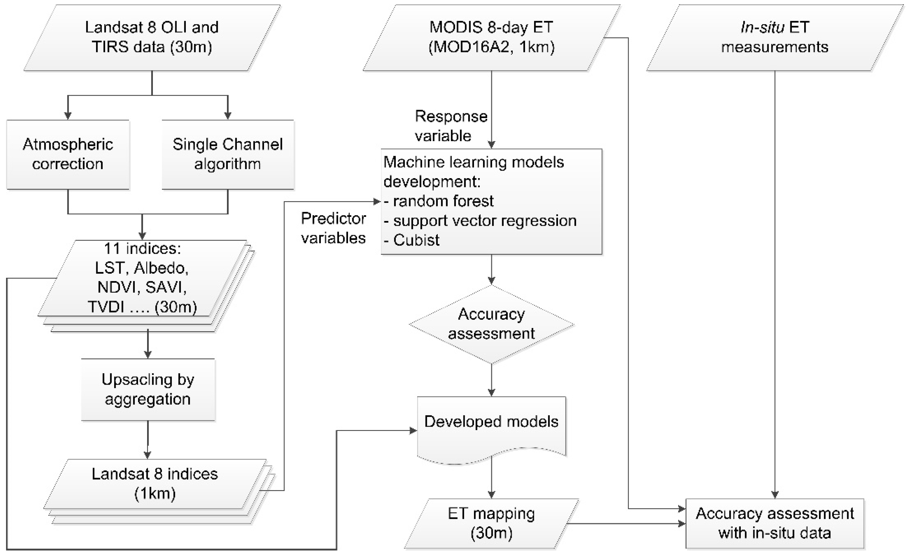
23,24]. The objective of this study is to develop a machine learning-based method in order to generate 8-day ET maps at 30 m resolution, based on MODIS 8-day ET product (MOD16A2) and Landsat 8 data, aiming to produce higher resolution ET that is consistent with the MODIS ET product. The method assumed that vegetation and surface wetness conditions do not change considerably within an 8-day interval. We examined three machine learning approaches—Cubist, Support Vector Regression (SVR), and Random Forest (RF)—for downscaling of MODIS 1 km 8-day ET product (MOD16A2) using eleven 30-m Landsat 8 data-derived variables (indices), including surface albedo, LST, Normalized Difference Vegetation Index (NDVI), Enhanced Vegetation Index (EVI), Soil Adjusted Vegetation Index (SAVI), Modified Soil Adjusted Vegetation Index (MSAVI), Normalized Difference Moisture Index (NDMI), Normalized Difference Water Index (NDWI), Depth of Landsat 8 OLI band 6 (D1609), Normalized Difference Infrared Index—Landsat 8 OLI band 7 (NDIIb7) and Temperature Vegetation Dryness Index (TVDI). Among the eleven indices, LST has been successfully used for ET estimation due to its sensitivity to local moisture status; surface albedo has been used as an input parameter for various SEB models; vegetation greenness indices including NDVI, EVI, SAVI and MSAVI are associated with growing status of vegetation; and wetness indices including NDWI, NDMI, D
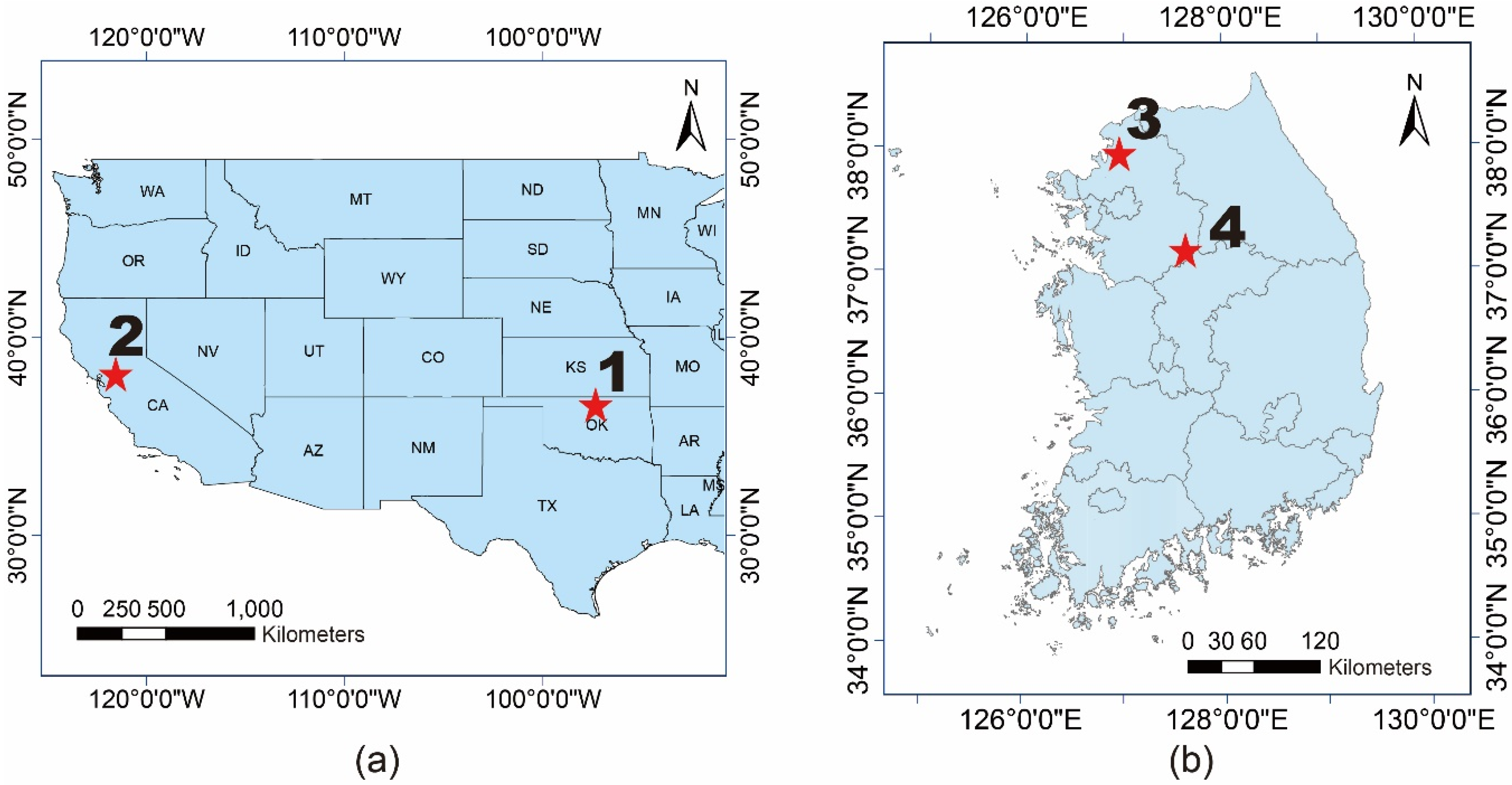
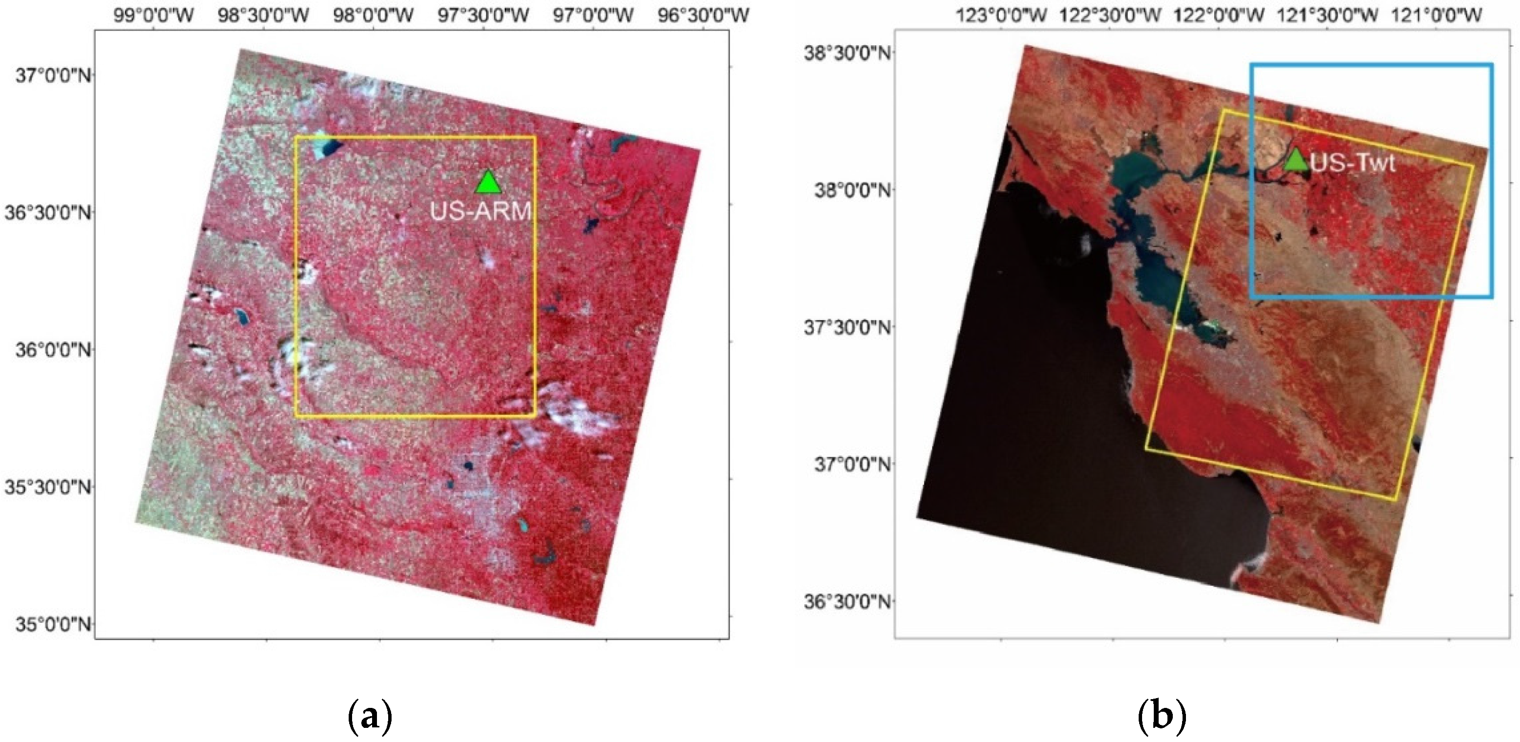
1609, and NDIIb7 are highly correlated with water consumption that is reflected from ET processes. The method assumed that vegetation and surface wetness conditions do not change considerably within an 8-day interval, and the growing status of vegetation is highly correlated with water consumption that is reflected from ET processes. Different from previous ET downscaling methods, the machine learning models in our study do not need to calculate Landsat-based ET and thus do not rely on the accuracy of meteorological parameters. The models were tested at four study sites within different climate zones in the United States and South Korea, and evaluated using in situ flux tower measurements.

2. Study Area and Data

2.1. Study Areas

Four study areas, including two sites in the United States and two sites in South Korea, were explored in this study (Figure 1). The two U.S. sites are located near Lamont, Oklahoma (Site 1: 97.89°W, 36.27°N) and Twitchell Island, California (Site 2: 121.65°W, 37.58°N), and feature two distinct climate conditions based on the Köppen–Geiger climate classification map [31]. Site 1 experiences a humid subtropical climate (Köppen climate map classified as Cfa) with hot, wet summers and cold, dry winters. The average temperature is around 16.3 °C and annual precipitation is around 880 mm. Twitchell Island is within the Sacramento-San Joaquin Delta approximately 100 km inland from the Pacific Ocean and a Mediterranean climate zone, with hot, dry summers, and cool, wet winters (Köppen climate map classified as Csb). The mean air temperature is 15.1 °C and the mean annual precipitation is 335 mm.
Two sites in South Korea are Seolmacheon in Paju (Site 3: 126.95°E, 37.93°N) and Cheongmicheon in Yeoju (Site 4: 126.65°E, 37.15°N). The climatic characteristics of the two sites are similar. Both are of humid climate and hot in summer while cold in winter. Annual mean temperature of the sites is about 11.5 °C and annual precipitation is about 1150 mm. While Seolmacheon is located in a mixed forest, Cheongmicheon is located in rice paddy fields.

2.2. Landsat 8 Imagery and MODIS ET Products

A total of 32 Landsat 8 Level 1 (L1T) images with minimum cloud cover (<5% within the study area) during the year 2013–2014 were obtained from USGS Global Visualization Viewer (http://glovis.usgs.gov/), including 11 images over Site 1 from 3 June 2013 to 25 August 2014; 15 images over Site 2 from 16 April 2013 to 9 August 2014, and three images over each of Sites 3 and 4 during the growing season (Figure 2, Table 1). Because of the geometric excellence of Landsat 8 OLI and TIRS images [32], all images had geometric accuracy, i.e., root mean square error (RMSE) less than 1 pixel. A subset of each image was extracted to cover a variety of land cover types and less non-vegetated area.
MODIS ET product, specifically MOD16A2, provides global ET, latent heat flux (LE), potential ET (PET), potential LE (PLE) datasets, and the quality control flag of ET (ET_QC) for each 8-day interval (5-day or 6-day for the end of the year) at 1 km resolution from the year 2000 to 2014 [33]. MOD16A2 ET is the sum of ET during each 8-day time periods within a year (mm/8 days, mm/5 days or mm/6 days for 361 composite data). In this study, the datasets covering Landsat image dates were selected, with starting dates of 1–4 days before the Landsat image was acquired (Table 1). ET and ET_QC layers were subset within the study area boundary, and the quality flag layer was used to exclude low quality ET. All ET products were re-projected to be the same projection system with Landsat 8 imagery, i.e., UTM WGS 1984 14N for Site 1, 10N for Site 2 and 52N for Sites 3 and 4.

2.3. In Situ ET Calculation

In situ ET measurements were obtained from AmeriFlux towers at the two U.S. sites and flux towers operated by the Hydrological Survey Centre at the South Korean sites. AmeriFlux is a network composed of over 110 sites across North and South America that continuously measure meteorological variables such as CO2, water and energy fluxes using an eddy covariance technique. In this study, each U.S. site has an AmeriFlux tower station, namely US Atmospheric Radiation Measurement Program Southern Great Plains Main (US-ARM SGP Main) at Site 1, and US Twitchell Island (US-Twt) at Site 2 (Figure 2a,b). US-ARM flux tower is located at an open cattle pasture surrounded by a rain fed winter wheat field [34]. Summer crops such as maize, soybean, or sorghum are commonly planted after wheat is harvested [34,35]. US-Twt site is a rice paddy field. Level 2 data with half-hourly flux measurements during 2013-2014 were downloaded and processed as higher level data is not available for recent years. Air temperature, relative humidity (RH) and air pressure (Pa) measurements were used to calculate water vapor for LST computation [36], and LE (W/m2) measurements were used to derive 8-day ET measurements (mm/8-day) following [10]. As the AmeriFlux tower observations are collected every 30 minutes, ET (mm/30 min) was first calculated as
λ = ( 2.501 0.002361 × T n ) × 10 6
E T n = L E n × 60.0 × 30.0 λ
where T n is air temperature for nth 30-minute observation in degree Celsius and λ is the latent heat of vaporization (J/kg). When the number of valid 30-minute measurements of LE and T n (N) is no less than 40, daily ET was calculated using Equation (3). When N is less than 40, daily ET was estimated by linear interpolation with the two nearest daily ET values. The 8-day ET is a sum of daily ET during an 8-day interval with the same starting date of MODIS ET product.
E T = n = 1 N E T n × 48 N
Similar to the AmeriFlux system, two flux towers in South Korea (i.e., Seolmacheon in Site 3 and Cheongmicheon in Site 4) measure meteorological and soil parameters and use an eddy covariance method to calculate ET (Figure 2c,d). The Seolmacheon flux tower was designed to observe ET over a mixed forest with trees of 30–50 years at an altitude of about 420 m, while the Cheongmicheon was constructed to monitor ET over agricultural lands in a rice paddy area at an altitude of 310 m.

3. Methodology

The ET downscaling method mainly consists of three components (Figure 3), including (1) derivation of eleven Landsat 8 data-based indicators that are associated with vegetation growth, surface temperature and moisture, and upscaling of the indicators so as to be consistent with the MODIS 8-day ET product; (2) development of machine learning models using samples with Landsat 8-derived indicators as predictor variables and MODIS 8-day ET as a response variable; and (3) generation of ET with 30 m resolution based on the developed models, and accuracy assessment through comparison between the downscaled ET, MODIS and in situ ET measurements.

3.1. Derivation and Upscaling of Landsat 8-Based Indices

3.1.1. Landsat 8 VIs Calculation

Surface albedo and vegetation indices were derived from Landsat 8 OLI surface reflectance. Although surface reflectance data for the Landsat 8 OLI sensor are provided from USGS, the internal atmospheric correction algorithm has not been published and validated [37]. Research has found that different atmospheric correction methods, such as Second Simulation of a Satellite Signal in the Solar Spectrum Vector (6SV), radiative transfer algorithm, Dark Object Subtraction (DOS) and Fast Line-of-sight Atmospheric Analysis of Hypercubes (FLAASH) algorithm do not produce significant differences in vegetation index calculation from Landsat 8 OLI data [27]. Therefore, in this study we adopted the FLAASH algorithm in ENVI software to perform atmospheric correction for the Landsat 8 images. Surface reflectance of bands 1–7 were used to calculate albedo and vegetation indices, and a brightness temperature of band 10 was used to generate LST. Cloud and cloud shadows were detected using the “Fmask” algorithm [38] in order to create a mask layer. The mask layer, in combination with Landsat 8 OLI L1T-provided Quality Assurance (QA) data were used to remove contamination by cloud/cirrus/shadow. Eight vegetation indices showing vegetation greenness and water content including NDVI, EVI, SAVI, MSAVI, NDMI, NDWI, NDIIb7, and D1609 were calculated from surface reflectance for each cloud-clear pixel (see Table 2 [39,40,41,42,43,44,45,46] for equations).

3.1.2. Landsat 8 Broadband Surface Albedo Estimation

To date, operational algorithms have not been developed for Landsat 8 OLI broadband surface albedo computation. Compared to its predecessors Landsat TM and ETM+ sensors, Landsat 8 OLI incorporates two additional spectral bands, one deep blue band (0.43–0.45 μm) and one shortwave infrared band (1.36–1.39 μm). Besides, reflective wavebands corresponding to the previous Landsat ETM+ bands have narrower waveband widths, i.e., different spectral response functions. Therefore, algorithms and parameters developed for albedo calculation for Landsat TM/ETM+ sensors cannot be directly used for the Landsat 8 OLI sensor. In this study, the albedo calculation strategy widely used for SEB models was employed [47], where broadband surface albedo is calculated as the integration of at-surface reflectance across the shortwave spectrum, as shown in Equation (4).
α =   b = 1 7 [ ρ b · w b ]
where α is albedo, ρ b is surface reflectance for a given band b, which can be derived from any atmospheric correction method such as FLAASH used in this study. w b is the weighting coefficient representing the surface solar radiation fraction within the spectral range for band b, and is calculated as:
w b =   L O b U P b R s λ · d λ 0.3 4 R s λ · d λ
where R s λ is at-surface spectral hemisphere solar radiation for wavelength λ (μm); and U P b and L O b are upper- and lower-wavelength bounds assigned to Landsat 8 band b, respectively. Table 3 lists the band settings of Landsat 8 OLI in comparison with Landsat 7 ETM+ sensor. Landsat 8 OLI Cirrus band (band 9: 1.36–1.39 μm) was not included in calculation due to its high absorption and low reflective characteristics.
Following similar procedures in [47], the Simple Model of the Atmospheric Radiative Transfer of Sunshine (SMARTS) radiative transfer model [48] was used for the calculation of at-surface solar radiation levels for three combinations of land elevations, precipitable water content, and solar angles. Regardless of the wide range of solar radiation settings, w b did not have significant change. Table 4 presents the calculated w b for Landsat 8 OLI in comparison with Landsat 7 ETM+ sensor.

3.1.3. Landsat 8 LST and TVDI Estimation

Although Landsat 8 TIRS sensor measures thermal infrared radiance with two bands (band 10 and band 11) located at 10 and 12 μm, significant calibration errors caused by stray light have been reported for band 11 [49]. As suggested by United States Geological Survey (USGS), a single channel algorithm by Jiménez-Muñoz et al. [50] was adopted to derive land surface temperature from band 10 in this study. Water vapor content required by the algorithm was derived from the measurements at weather stations or the MODIS water vapor product (MOD05L2 Collection 5.1) if weather station measurements were not available within the study area [36].
TVDI, which represents water stress of vegetation, was estimated on the basis of the triangular shape of LST vs. NDVI scatter plots [51].
T V D I   =   T s   T s m i n a +   b · N D V I   T s m i n
where T s is LST for each pixel in the image, T s m i n is the minimum LST, i.e., wet edge in the LST-NDVI space. Coefficients a and b are determined by a linear fit between maximum LST for a given NDVI ( T s m a x ) and NDVI at the dry edge [51].

3.1.4. Upscaling of Landsat 8 Indices

Landsat 8 data-derived indicators were upscaled to 1 km resolution by means of a simple aggregation approach. First, MODIS 8-day 1 km ET product (MOD16A2) was re-projected with the same projection system as Landsat 8 data. For each indicator, pixels within each MODIS 1 km grid were averaged to generate Landsat 1 km indicators. If a considerable amount of 30 m pixels (>30%) were covered with cloud/cirrus/cloud shadow within a 1 km grid, the grid was excluded from modeling. Ke et al. [27] has shown that the simple aggregation method produced good consistency between Landsat 8 derived NDVI and MODIS NDVI at MODIS resolution. MOD16A2 QA masks were also used to remove grids with low quality caused by cloud/aerosol states or algorithm failure [33].

3.2. Machine Learning-Based Downscaling Models

Three machine learning algorithms including Cubist, Support Vector Regression (SVR) and Random Forest (RF) were examined in this study. Cubist is a software package that implements a modified regression tree algorithm, which combines instance- and model-based techniques to create rule-based multivariate regression models from training data [52]. It allows overlap between multivariate regression models, thus predictions from multiple rules are averaged to produce the final output. Cubist has been widely used in different applications of remote sensing, such as biomass estimation, impervious surface quantification, drought monitoring, water quality estimation, and land cover estimation [53,54,55,56].
SVR is a regression version of Support vector machines (SVMs). The basic principle of SVM is that independent variables are mapped to a higher dimensional space where nonlinear correlations are transformed to be linearly separable using kernel functions, and the optimal linear separator is selected to maximize the margin between classes [57]. SVR, as an extension of SVM, uses the same principles as SVM for classification, while it can produce real numbers as output given a set of independent input variables by defining a margin of tolerance (ε). Both SVM and SVR have been proven robust for classification and the estimation of continuous properties in remote sensing [58,59,60,61,62,63,64]. In this study, LibSVM (version 3.20) tools developed by Chang and Lin [65] were adopted to implement SVR, for which the radius basis function (RBF) kernel was used and the optimal combination of parameters such as cost, gamma and ε were selected using a grid search approach.
RF is an improved algorithm based on a classification and regression trees (CART) method, by combining a large set of CARTs in an ensemble. It has been widely used for various remote sensing applications for both classification and regression [66,67,68]. Compared to the CART algorithm, RF uses a bootstrap aggregating technique to improve model performance. Each tree is built from a random subset of training data with a random subset of predictor variables, and the aggregation of output from many trees may smooth the variance between trees and yield more accurate prediction results [69]. Variable importance is obtained by the percentage increase in the mean squared error (MSE), which is calculated using out-of-bag (OOB) data when each variable is permuted. In this study, randomForest add-on package provided in R statistical software was used to implement the method.
Using the eleven upscaled 1 km Landsat indices as predictor variables and MODIS 1 km ET product as the response variable, prediction models were established based on Cubist, SVR and RF algorithms, respectively. The developed models were then applied to the eleven 30 m Landsat indices in order to generate 30 m ET product. In order to evaluate the model performances, ten-fold cross validation with fixed subsets of samples was conducted for each model, and the average RMSE and relative RMSE (rRMSE) as a percentage of mean MODIS 8-day ET of validation datasets were assessed and compared. The developed machine learning models were then applied to the original 30 m Landsat indicator layers to predict downscaled ET at 30 m resolution. The models were also applied to the upscaled indicators to create Landsat-modeled 1 km ET. The downscaled 30 m ET was then compared with MODIS 1 km ET and Landsat modeled 1 km ET in terms of the ET spatial patterns. The predicted 30 m ET was aggregated to 1 km resolution and compared to MODIS ET. All four products, including MODIS 1 km ET, Landsat-downscaled 30 m ET, Landsat-modeled 1 km ET, and Landsat-aggregated 1 km ET were assessed using in situ ET measurements.

4. Results

4.1. Results from Three Machine Learning Algorithms

Among all three models, SVR models resulted in the lowest performances, as the RMSE and rRMSE were always the highest at all study sites (Figure 4). RF yielded similar or slightly better performances than Cubist, with RMSE less than 2.5 mm/8 days for US sites and 5.7 mm/8 days for Korean sites; rRMSEs were less than 20% at the US sites and less than 15% at Korea sites, which is within the range of the MODIS ET product accuracy (rRMSE around 25%) [10]. Performances of all models have similar temporal patterns, with increasing errors (both RMSE and rRMSE) during growing seasons (June–September) and decreasing errors during leaf-off seasons (October–December).
Figure 5 shows the average importance of the eleven Landsat indicators resulting from all RF models and their ranks. Importance of a variable is measured by the increase in MSE when the variable is permuted. Greater increase in MSE indicates higher importance of the variable. Table 5 shows the mean and standard deviation of linear correlation coefficients ( ρ ) between Landsat indicators and MODIS ET calculated at all dates or only during growing seasons. From Figure 5 and Table 5, the variable importance in RF models was largely consistent with the correlations between the variables and MODIS ET. Among the eleven indictors, NDVI, EVI, and SAVI that are related to vegetation greenness and growth conditions were ranked the most important in ET modeling. Permuting values of NDVI could lead to as much as a 7.2 mm/8 days ET bias. The correlation coefficients between these variables and MODIS ET were also highest with positive relationships ( ρ > 0.69 when averaged at all dates and ρ > 0.73 during growing seasons, p-value < 0.0001).
Variables representing vegetation moisture status including NDIIb7 and NDWI were ranked the fourth and fifth. As is shown in Table 5, correlations between NDIIb7, NDWI and MODIS ET were slightly weaker than NDVI/EVI/SAVI but still strong and significant ( ρ = 0.68 and −0.67, respectively, for all seasons and ρ = 0.79 and −0.76 for growing seasons). LST and TVDI are also negatively related to ET as increasing temperature usually corresponds to dry conditions resulting in less evapotranspiration. Although previous studies have shown that temperature-related variables have a dominant impact on satellite-based daily ET estimation, the correlation coefficients between LST and ET are only −0.59 on average in our study and those between TVDI and ET were only −0.32 when all seasons were considered. LST/TVDI were overall ranked less important than vegetation greenness and moisture indices. However, during growing seasons the relationships between LST/TVDI and ET were much stronger, as the correlation coefficients increased to −0.73 and −0.60, respectively, and the standard deviations declined. Albedo has little impact on the modeling results. The relationship between albedo and ET was weak ( ρ = −0.38 for all seasons and −0.44 for growing season). The modified SAVI (MSAVI) was not superior over SAVI in this study, as the correlation was weaker and was not identified as an important variable.

4.2. Agreement between Landsat and MODIS ET

As RF outperformed SVR and it produced similar or slightly better accuracy than Cubist, it was used to generate the downscaled 30 m ET and Landsat modeled 1 km ET. In order to evaluate the overall agreement of Landsat downscaled ET against MODIS ET, the 30 m product was aggregated to 1 km grids (Landsat-aggregated 1 km ET), and RMSE and rRMSE were calculated for each site. As shown in Figure 6, RMSE of Landsat-aggregated 1 km ET was within 2 mm/8 days and rRMSE within 23% at Site 1. Site 2 produced slightly higher RMSE (0.8–2.9 mm/8 days) and rRMSE (15%–26%). Korean sites have higher RMSE and similar rRMSE as US sites. The average rRMSE from the four sites is 22%. Sites 1 and 2 showed obviously similar temporal trends, as the aggregated ET had a decreasing agreement with MODIS ET during the growing season compared to leaf-off season. The agreement was slightly lower than, if not similar as, that between the Landsat modeled 1 km ET and MODIS ET shown in Figure 4. This means that the model performance could be used as an indicator to explain the resultant accuracy of downscaled ET with MODIS ET as reference data.
Figure 7 and Figure 8 show time series of the ET maps at the northeast part of Site 2 (US-Twt) and the southwest part of Site 4 (Cheongmicheon) through 2013 and the corresponding land cover types. Both Landsat modeled 1 km and Landsat downscaled 30 m ET showed very similar spatiotemporal patterns as MODIS ET. At cropland, which is mainly irrigated in Site 2, ET increased from April to July, and then decreased until the end of the year. ET in grassland showed a decreasing trend since April. As grass growth in this area is mainly controlled by the amount of precipitation, it is expected that ET is lower during the hot and dry summer. Spatial variation of ET at cropland was higher than the other vegetated land covers for all three products, and at cropland the Landsat downscaled product showed even more detailed spatial distribution of ET than MODIS and the Landsat modeled 1 km ETs. Since only three dates were available for Site 4, the temporal patterns of ET were not captured in details. However, ET at cropland was a bit lower than that in forests in the middle of the growing season (i.e., June) while ET was very low during the off-growing season (i.e., November) regardless of land cover type. The good agreement between Landsat and MODIS ET in terms of spatial and temporal patterns proved the potential of our downscaling approach.

4.3. Spatial Variation of the Downscaled ET Product

It is obvious that the Landsat-scale ET map in Figure 7 and Figure 8 showed more spatial details than coarse resolution ET. Zoomed views of Landsat downscaled ET at Site 2 (Figure 9) also demonstrated that the product was able to represent the spatiotemporal dynamics of ET at the patch level, with different patches showing varying trends of ET change.
In order to evaluate the improvement of spatial information represented by the downscaled ET, the differences between the 30 m and 1 km MODIS ETs within the corresponding 1 km grids was calculated and the statistics of the differences was analyzed for each land cover type. First, a 1 km land cover layer was generated using 30 m land cover products. The USGS National Land Cover Database (NLCD) 2011 [70] was used for US sites and three land cover products (MODIS Global 500m Terra and Aqua combined land cover product (MCD12Q1 IGBP) [71], European Space Agency (ESA) Global Land Cover Map 2009 product (GlobCover 2009) [72], and the Finer Resolution Observation and Monitoring of Global Land Cover (FROM-GLC) [73] were combined for Korea sites to ensure accurate land cover information [27]. The three products were combined to create a new ensemble 30 m land cover data only using the pixels that agreed from all three land cover layers. Grids with pure land cover types, i.e., a single land cover occupying over 80% of the 1 km grid area were selected for further analysis. Boxplots in Figure 10 show the distribution of the differences between 30 m Landsat downscaled ET and MODIS ET within crop, forest, grass, and shrub land. For all sites, the median of the differences was around zero, indicating an overall unbiased estimation of ET using MODIS ET as a reference. Dispersion of the biases against MODIS ET increased from spring to summer and decreased during winter, implying that the downscaled ET revealed a higher spatial variation during growing seasons. At Site 1, the majority of the differences (25th–75th percentile) was within ±5 mm/8 days, and the extreme difference values were around ±10 mm/8 days. Cropland and forests showed a slightly greater dispersion of the differences than grassland. At Site 2, the difference values were on average within ±5 mm/8 days; the extreme values were on average ±20 mm/8 days at croplands and forest, and ±6 mm/8 days at grassland and shrub area. Sites 3 and 4 showed a similar pattern. For both sites, the majority of the differences (25th–75th percentile) were within ±10 mm/8 days, and the extreme difference values were around ±20 mm/8 days. Dispersion of the biases considerably decreased during the leaf-off season for Site 4, while it was maximized in the middle of the growing season for Site 3.

4.4. Comparisons between Satellite-Based and in Situ ET

Time series of satellite-based ET and in situ observations at the flux towers (US-ARM, US-Twt, Seolmacheon, and Chungmicheon) within the four study sites are summarized in Figure 11. At the four sites, both satellite-based and in situ ETs showed a similar seasonal trend, with a peak season around July and a low season in December at Sites 1, 2, and 4, and ET peak was found to be in the middle of the growing season at Site 3. Compared to the other sites, the flux tower at Site 2 (US-Twt) observed greater ET in growing seasons. This is because the flux tower is located within a rice paddy that consumes a greater amount of water than the wheat does at Site 1 (similarly rice paddy at Site 4). Each year, the field is flooded after rice is planted in spring, and drained when rice is harvested in early fall. Thus, ET experiences a rapid rise from April to June and a sharp descent from September.
Although satellite-based products captured the temporal trend of ET variation at the four study sites, the values of ET had large discrepancies from the in situ ET measurements, especially during growing seasons. Figure 11a, b, and d show a large underestimation of ET at the crop sites, especially for the MODIS-based, Landsat modeled 1 km, and Landsat aggregated 1 km products, with the bias as great as −20 mm/8 days. The downscaled 30 m ET is similar to MODIS ET at US-ARM (Site 1, during the year 2013) and Cheongmicheon (Site 4), while at US-Twt (Site 2) it is on average 13mm/8days higher than MODIS ET during growing seasons, which is closer to in situ ET. Further examination indicates that compared to Sites 1 and 4, the crop patches are more heterogeneous within a 1 km grid around the flux measurement tower at Site 2 (Figure 11f). The measurement tower is located within a rice patch, with higher vegetation greenness and wetness values and lower LST observation compared to the corn, alfalfa and fallow/idle crop patches surrounding the tower [74], thus higher ET estimates than the 1 km averaged ET within the MODIS 1 km grid. The higher and more accurate downscaled ET estimation at US-Twt site shows that the downscaling models could capture the ET spatial variation. Although it would be ideal to select homogeneous lands for our model evaluation, US-ARM and US-Twt are the only crop sites that provide flux measurements going up to 2014, and they represent typical climate types. Cheongmicheon (Site 4) is surrounded by rice paddy fields and a small portion of forested areas. Cheongmicheon showed a similar pattern with Sites 1 and 2, but the differences between the satellite-based and in situ ETs in Site 4 were smaller (~10 mm/8 days for the growing season and ~1 mm/8 days for the off-growing season) than in Sites 1 and 2, which could be due to relatively homogeneous crop areas and nearby forests. Unlike other sites, satellite-derived ETs were higher than in situ ET measurements for all three dates in the growing season at Site 3 (Figure 11c), where forest is the dominant land cover. Hu et al. [11] reported similar findings that the MOD16 ET product tends to overestimate forest ET mainly due to high LAI values used as input to ET estimation models. It was not able to look into seasonal variation, as there were only three dates of satellite-derived ETs all of which were from the growing season. While there were also three dates of satellite-derived ETs in Site 4, one was from the growing season and the other two from the off-growing season. Both in situ and satellite-derived ET showed a similar seasonal pattern at Sites 1 and 2.
Figure 12 shows the scatterplots of satellite-based ET estimates against in situ observations at each of the four sites, and Table 6 lists their linear agreement. Note that linear regression was not calculated for Sites 3 and 4 because there were only three measurements for the sites. At Site 1, downscaled ET yielded the highest R2 (0.76) and lowest RMSE (11.8 mm/8 days) compared to coarse resolution products. At Site 2, although downscaled ET produced lower R2 than MODIS ET, it still gave the lowest RMSE.

5. Discussion

5.1. Novelty, Performances and Opportunities

In this paper, machine learning approaches were first introduced for ET downscaling from coarse resolution to fine resolution by combining MODIS 8-day ET product and Landsat 8-derived eleven indicators. The rRMSEs of RF models were less than 20% and within the error range of the MODIS ET product (rRMSE around 25%), indicating the reliability of the downscaling model. Among the eleven indicators, vegetation greenness-related indices such as NDVI/EVI/SAVI were the most important variables used in the machine learning modeling. In Penman–Monteith model that was used to generate MOD16 ET products, remotely-sensed LAI is an important input parameter for quantification of wet canopy surface evaporation and plant transpiration [33]. As LAI and NDVI/EVI/SAVI are highly correlated, it is reasonable that these variables were highly important. These indices have also long been recognized as important indicators for ET estimation, especially at crop areas that were dominant land cover types in study Sites 1, 2 and 4. NDVI is on average the most important indicator among the VIs. Although NDVI is known to have saturation issues and it can be influenced by soil background, the use of EVI and other vegetation greenness related indices such as SAVI could help to avoid these issues and ensures the reliability of the models. Vegetation moisture-based indicators such as NDIIb7 and NDWI were also important because these variables describe soil moisture and leaf water content, higher leaf moisture results in greater amount of water transpired from leaves, especially during growing seasons. Interestingly, LST-related indicators were less important. Unlike SEB models that rely on LST to derive ET, the Penman–Monteith model did not use remotely sensed LST as an input. On the other hand, LST derived from Landsat 8 imagery only represents the instant thermal conditions at the image acquisition date/time. Although our investigation showed that the instant Landsat-derived LST had high correlation with the MODIS 8-day average LST product (MOD11A2) ( ρ > 0.8 and mean R2 = 0.83), the surface temperature can vary considerably during the 8-day period. Therefore, it is not surprising that LST has less of a contribution to the modeling of 8-day aggregated ET.
Our results showed that the downscaled ET is overall consistent with MODIS ET product, and it demonstrates detailed spatial variation and temporal trend at 30 m resolution. The downscaling approach assumes that Landsat-derived indicators characterize vegetation conditions during each 8-day period. The overall consistency between downscaled and MODIS ET proved that this assumption is reasonable even when the resolution of MODIS ET product is over 1000 times (33 × 33) coarser than Landsat data. Greater variation of the downscaled ET over cropland was observed as crop ET varies significantly with irrigation and growth. This also demonstrated the capability of the product to represent the spatial and temporal heterogeneity of ET. The ET estimates have better agreement with in situ measurements, especially at Site 2 where ET heterogeneity is high within 1 km grids. Because the downscaling models rely on the MODIS ET estimation, the accuracy of the MODIS product highly impacts the finer-resolution estimation. With the improved accuracy of coarse resolution global or regional ET products, it is expected that our downscaling approach can achieve better performance in various regions with different climate and environmental characteristics.
The downscaling method is easy to implement; it does not require computation of Landsat daily ET, hence does not need parameter tuning for ET estimation models such as SEB, and the method is not impacted by the accuracy of meteorological parameters such as solar radiation and wind speed. All indicators used in the machine learning models can be easily derived based on Landsat 8 OLI and TIRS data. Because the satellite-based indicators are spatially explicit, the method can be applied over large areas or basins for ET estimation. It is also expected that this approach can also be applied to the downscaling of daily MODIS ET or ET from other coarse-resolution satellites such as MERIS.

5.2. Challenges

One major limitation of the proposed approach is that the accuracy of downscaled ET is greatly impacted by the accuracy of coarse-resolution ET. As many methods have been developed for improving MODIS ET [75,76], better MODIS ET estimation is expected to increase the accuracy of the downscaled product. Another disadvantage of the approach is that downscaled ET can only be produced on cloudless image acquisition days. In areas with more frequent cloud cover, such as South Korea, the approach might not be able to describe the temporal trends of ET at higher spatial resolution. As Landsat 8 collects images in an 8-day offset from Landsat 7, our approach may provide ET at higher temporal resolution using the combination of the two datasets. In our future research, spatial-temporal fusion of Landsat data and MODIS ET will be explored to increase the temporal resolution of downscaled ET. The proposed approach may require post processing over the areas overlapped between adjacent Landsat scenes or the boundary areas of MODIS tiles where there could be spatial discrepancy of ET estimates. One possible solution would be to use merging algorithms typically used to mosaic images considering spatiotemporal variations of ET estimates. An alternative is to use fusion algorithms that are often used for downscaling such as Spatial and Temporal Adaptive Reflectance Fusion Model (STARFM; [22,77]) to mitigate the variations of ET estimates over such overlapped areas.

6. Conclusions

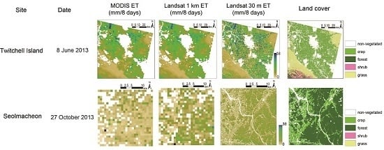
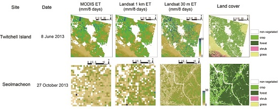
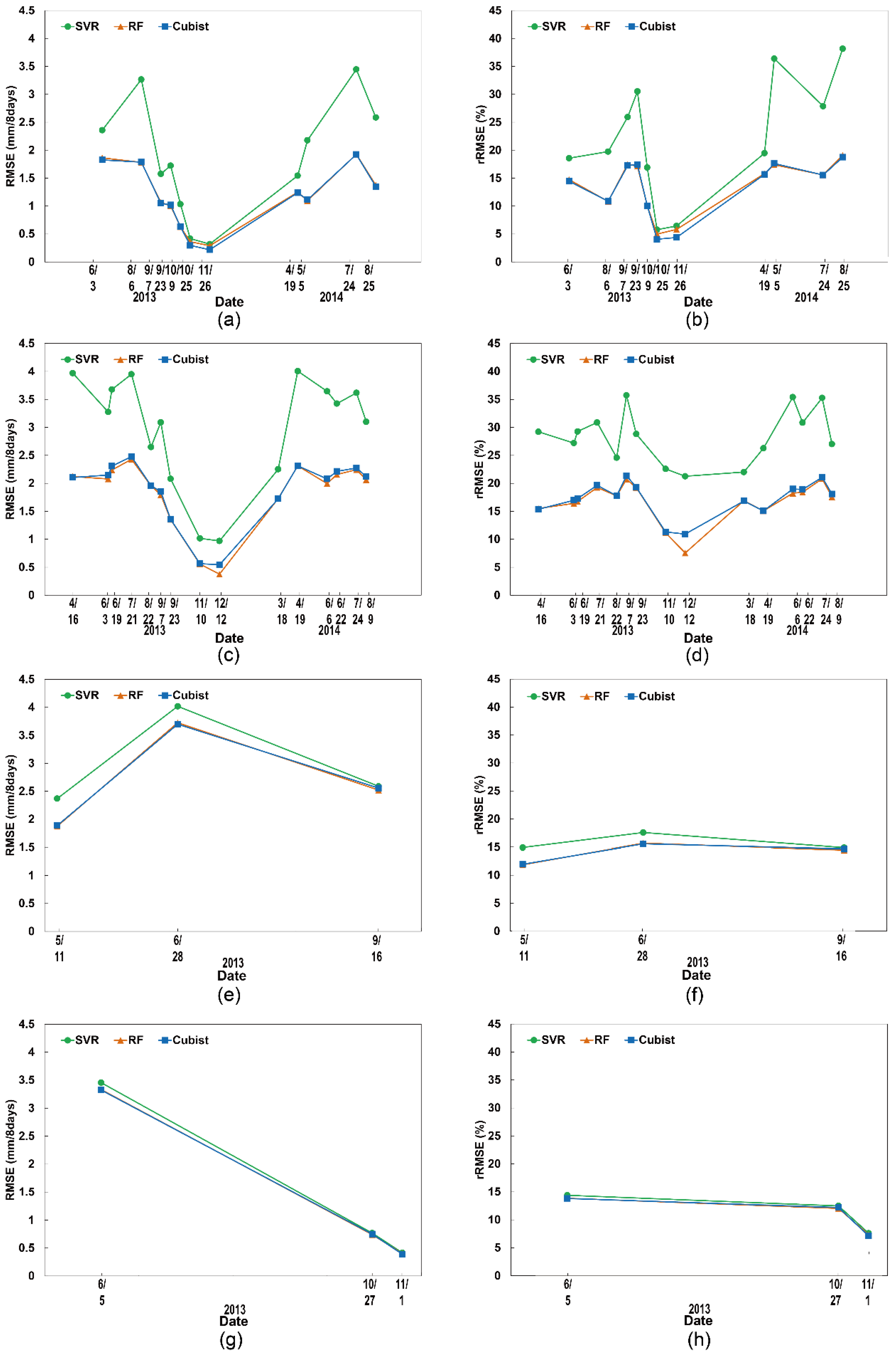
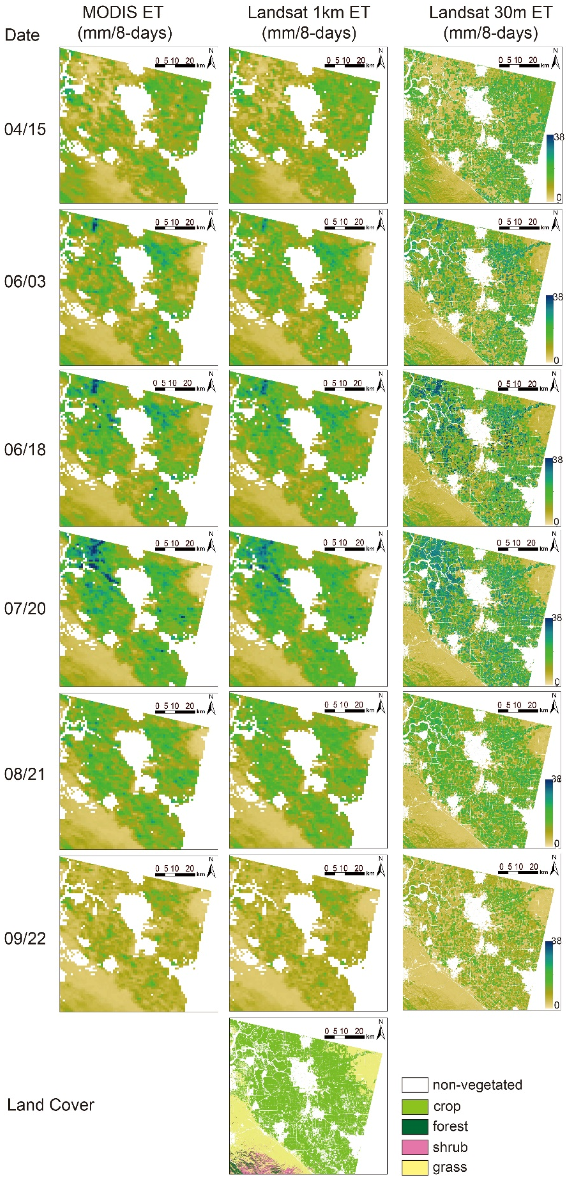
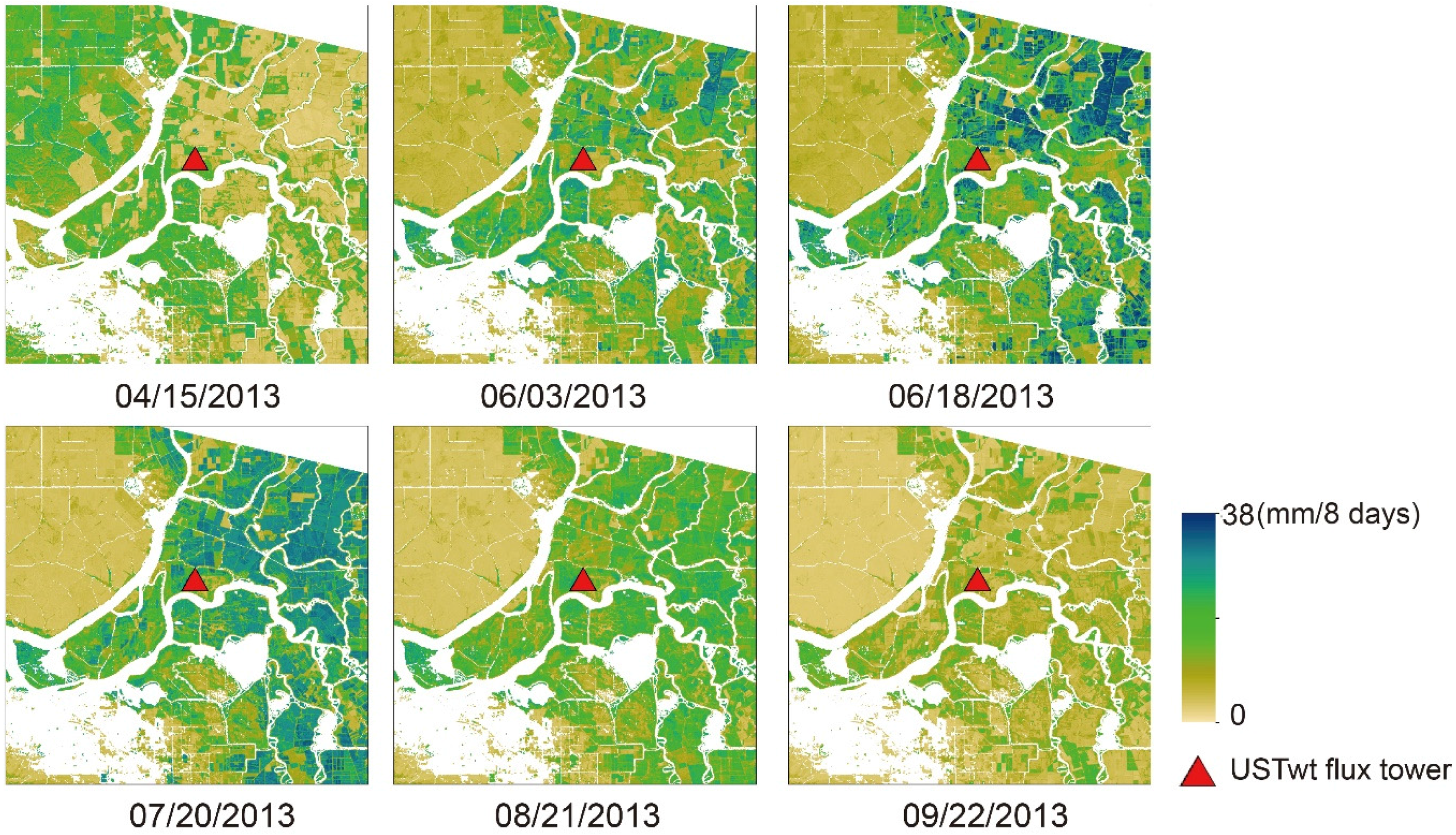
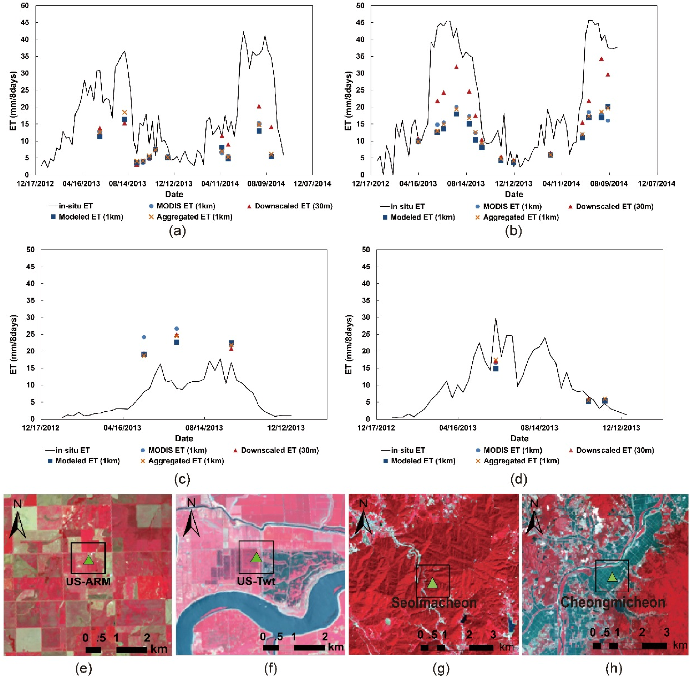
In this study, we proposed a machine learning-based method for MODIS ET downscaling with Landsat 8 data. Eleven indicators, including albedo, LST, and VIs such as NDVI, EVI, SAVI, MSAVI, NDMI, NDWI, D1609, NDIIb7 and TVDI, derived from Landsat 8 data, were used as predictor variables and MODIS 8-day 1 km ET product (MOD16A2) as a response variable to build machine learning models. Among the three machine learning algorithms including SVR, Cubist, and RF examined, RF and Cubist resulted in higher model accuracies. rRMSEs from RF models were less than 20% for the four study sites in the US and South Korea, which were within the error range of the MODIS ET product (rRMSE around 25%). The variable importance analysis showed that vegetation growth-related indicators such as NDVI, EVI, and SAVI were most important in 8-day ET modeling by RF, while vegetation moisture-based indicators such as NDIIb7 and NDWI had slightly lower importance. LST-related indicators representing temperature at the time of image acquisition were less important than either vegetation greenness or wetness indicators. The predicted Landsat downscaled ET had an overall good agreement with MODIS ET, as the average rRMSE was around 22%. The downscaled ET product showed a similar temporal trend as MODIS ET. In addition, the product demonstrated higher spatial details; especially in crop areas, the downscaled product could represent ET variation at patch scale. Neither MODIS ET nor Landsat downscaled ET product yielded a very good agreement with in situ ET probably because of land cover heterogeneity around flux tower sites, however, the downscaled ET estimates were closer to in situ observations (R2 = 0.76 and 0.77, RMSE = 11.8 and 12.5 mm/8 days for Site 1 and Site 2, respectively). The results showed the potential of using machine learning approaches for ET downscaling considering their effectiveness and ease of implementation. Our next study will explore spatial-temporal fusion methods that combine the advantages of high spatial resolution of Landsat data and high temporal resolution of MODIS ET in order to generate 8-day ET at 30 m resolution.

Acknowledgments

This research was supported by the Space Technology Development Program and Technology Development Program to Solve Climate Changes through the National Foundation of Korea (NRF) funded by the Ministry of Science, ICT, & Future Planning of Korea (Grant: NRF-2013M1A3A3A02042391, NRF-2014M1A3A3A03034799, and NRF-2012M1A2A2671851). The research was also supported by National Natural Science Foundation of China (Grant: 41401493; 41130744) and 2015 Beijing Nova Program (xx2015B060).

Author Contributions

Yinghai Ke led manuscript writing and contributed to the data analysis and research design. Jungho Im supervised this study, contributed to the research design and manuscript writing and served as the corresponding author. Seonyoung Park contributed to the data analysis and discussion of the results. Huili Gong contributed to the discussion of the results and manuscript writing.

Conflicts of Interest

The authors declare that there are no conflicts of interest.

References

  1. Anderson, M.C.; Allen, R.G.; Morse, A.; Kustas, W.P. Use of Landsat thermal imagery in monitoring evapotranspiration and managing water resources. Remote Sens. Environ. 2012, 122, 50–65. [Google Scholar] [CrossRef]
  2. Wang, S.; Pan, M.; Mu, Q.; Shi, X.; Mao, J.; Brümmer, C.; Jassal, R.S.; Krishnan, P.; Li, J.; Black, T.A. Comparing evapotranspiration from eddy covariance measurements, water budgets, remote sensing, and land surface models over Canada. J. Hydrometeorol. 2015, 16, 1540–1560. [Google Scholar] [CrossRef]
  3. Bastiaanssen, W.G.M.; Menenti, M.; Feddes, R.A.; Holtslag, A.A.M. A remote sensing surface energy balance algorithm for land (SEBAL): 1. Formulation. J. Hydrol. 1998, 198–213. [Google Scholar] [CrossRef]
  4. Bastiaanssen, W.G.M.; Pelgrum, H.; Wang, J.; Ma, Y.; Moreno, J.F.; Roerink, G.J. A remote sensing surface energy balance algorithm for land (SEBAL): 2. Validation. J. Hydrol. 1998, 213–229. [Google Scholar] [CrossRef]
  5. Allen, R.G.; Tasumi, M.; Morse, A.; Trezza, R.; Wright, J.L.; Bastiaanssen, W. Satellite-Based Energy Balance for Mapping Evapotranspiration with Internalized Calibration (METRIC)—Applications. J. Irrig. Drain. E-ASCE 2007, 133, 395–406. [Google Scholar] [CrossRef]
  6. Norman, J.M.; Anderson, M.C.; Kustas, W.P.; French, A.N.; Mecikalski, J.; Torn, R.; Diak, G.R.; Schmugge, T.J.; Tanner, B.C.W. Remote sensing of surface energy fluxes at 101-m pixel resolution. Water Resour. Res. 2003, 39, 1221–1237. [Google Scholar] [CrossRef]
  7. Su, Z. The Surface Energy Balance System (SEBS) for estimation of turbulent heat fluxes. Hydrol. Earth Syst. Sci. 2002, 6, 85–99. [Google Scholar] [CrossRef]
  8. Cleugh, H.A.; Leuning, R.; Mu, Q.; Running, S.W. Regional Evaporation Estimates from flux tower and MODIS satellite data. Remote Sens. Environ. 2007, 106, 285–304. [Google Scholar] [CrossRef]
  9. Mu, Q.; Heinsch, F.A.; Zhao, M.; Running, S.W. Development of a global evapotranspiration algorithm based on MODIS and global meteorology data. Remote Sens. Environ. 2007, 111, 519–536. [Google Scholar] [CrossRef]
  10. Mu, Q.; Zhao, M.; Running, S.W. Improvements to a MODIS global terrestrial evapotranspiration algorithm. Remote Sens. Environ. 2011, 115, 1781–1800. [Google Scholar] [CrossRef]
  11. Hu, G.; Jia, L.; Menenti, M. Comparison of MOD16 and LSA-SAF MSG evapotranspiration products over Europe for 2011. Remote Sens. Environ. 2015, 156, 510–526. [Google Scholar] [CrossRef]
  12. Ghilain, N.; Arboleda, A.; Gellens-Meulenberghs, F. Evapotranspiration modelling at large scale using near-real time MSG SEVIRI derived data. Hydrol. Earth Syst. Sci. 2011, 15, 771–786. [Google Scholar] [CrossRef]
  13. Yang, Y.; Guan, H.; Shang, S.; Long, D.; Simmons, C.T. Toward the use of the MODIS ET product to estimate terrestrial GPP for nonforest ecosystems. IEEE Geosci. Remote Sens. 2014, 11, 1624–1628. [Google Scholar] [CrossRef]
  14. Mu, Q.; Zhao, M.; Kimball, J.S.; McDowell, N.G.; Running, S.W. A remotely sensed global terrestrial drought severity index. B. Am. Meteorol. Soc. 2013, 94, 83–98. [Google Scholar] [CrossRef]
  15. Műnch, Z.; Conrad, J.; Gibson, L.; Palmer, A.; Hughes, D. Satellite earth observation as a tool to conceptualize hydrogeological fluxes in The Sandveld, South Africa. Hydrogeol. J. 2013, 21, 1053–1070. [Google Scholar] [CrossRef]
  16. Beigi, E.; Tsai, F. GIS-Based water budget framework for high-resolution groundwater recharge estimation of large-scale humid regions. J. Hydrol. Eng. 2014, 19, 5014004. [Google Scholar] [CrossRef]
  17. Momm, H.; Easson, G.; Bingner, R.; Wilcox, D. Evaluation of the use of remotely sensed evapotranspiration estimates into AnnAGNPS pollution model. Ecohydrology. 2011, 4, 650–660. [Google Scholar] [CrossRef]
  18. Hong, S.; Hendrickx, J.M.H.; Borchers, B. Down-scaling of SEBAL derived evapotranspiration maps from MODIS (250 m) to Landsat (30 m) scales. Int. J. Remote Sens. 2011, 32, 6457–6477. [Google Scholar] [CrossRef]
  19. Singh, R.; Senay, G.; Velpuri, N.; Bohms, S.; Verdin, J. On the downscaling of actual evapotranspiration maps based on combination of MODIS and Landsat-based actual evapotranspiration estimates. Remote Sens. 2014, 6, 10483. [Google Scholar] [CrossRef]
  20. Bhattarai, N.; Quackenbush, L.J.; Dougherty, M.; Marzen, L.J. A simple Landsat–MODIS fusion approach for monitoring seasonal evapotranspiration at 30 m spatial resolution. Int. J. Remote Sens. 2015, 36, 115–143. [Google Scholar] [CrossRef]
  21. Cammalleri, C.; Anderson, M.C.; Gao, F.; Hain, C.R.; Kustas, W.P. A data fusion approach for mapping daily evapotranspiration at field scale. Water Resour. Res. 2013, 49, 4672–4686. [Google Scholar] [CrossRef]
  22. Cammalleri, C.; Anderson, M.C.; Gao, F.; Hain, C.R.; Kustas, W.P. Mapping daily evapotranspiration at field scales over rainfed and irrigated agricultural areas using remote sensing data fusion. Agr. Forest Meteorol. 2014, 186, 1–11. [Google Scholar] [CrossRef]
  23. Ha, W.; Gowda, P.H.; Howell, T.A. A review of downscaling methods for remote sensing-based irrigation management: Part I. Irrig. Sci. 2013, 31, 831–850. [Google Scholar] [CrossRef]
  24. Ha, W.; Gowda, P.H.; Howell, T.A. A review of potential image fusion methods for remote sensing-based irrigation management: Part II. Irrig. Sci. 2013, 31, 851–869. [Google Scholar] [CrossRef]
  25. Wang, J.; Sammis, T.W.; Gutschick, V.P.; Gebremichael, M.; Miller, D.R. Sensitivity analysis of the Surface Energy Balance Algorithm for Land (SEBAL). T Asabe. 2008, 52, 801–811. [Google Scholar] [CrossRef]
  26. Mokhtari, M.H.; Ahmad, B.; Hoveidi, H.; Busu, I. Sensitivity analysis of METRIC–based evapotranspiration algorithm. Int. J. Environ. Res. 2013, 7, 407–422. [Google Scholar]
  27. Ke, Y.; Im, J.; Lee, J.; Gong, H.; Ryu, Y. Characteristics of Landsat 8 OLI-derived NDVI by comparison with multiple satellite sensors and in situ observations. Remote Sens. Environ. 2015, 164, 298–313. [Google Scholar] [CrossRef]
  28. Ghosh, S.; Mujumdar, P.P. Statistical downscaling of GCM simulations to streamflow using relevance vector machine. Adv. Water Resour. 2008, 31, 132–146. [Google Scholar] [CrossRef]
  29. Kaheil, Y.H.; Gill, M.K.; McKee, M.; Bastidas, L.A.; Rosero, E. Downscaling and assimilation of surface soil moisture using ground truth measurements. IEEE Trans. Geosci. Remote Sens. 2008, 46, 1375–1384. [Google Scholar] [CrossRef]
  30. Im, J.; Park, S.; Rhee, J.; Baek, J.; Choi, M. Downscaling of AMSR-E soil moisture with MODIS products using machine learning approaches. Environ. Earth Sci. under review.
  31. Kottek, M.; Grieser, J.; Beck, C.; Rudolf, B.; Rubel, F. World map of the Köppen-Geiger climate classification updated. Meteorol. Z. 2006, 15, 259–263. [Google Scholar] [CrossRef]
  32. Storey, J.; Choate, M.; Lee, K. Landsat 8 operational land imager on-orbit geometric calibration and performance. Remote Sens. 2014, 6, 11127. [Google Scholar] [CrossRef]
  33. Mu, Q.; Zhao, M.; Running, S.W. Algorithm Theoretical Basis Document: MODIS Global Terrestrial Evapotranspiration (ET) Product (NASA MOD16A2/A3) Collection 5. 2013. NASA Headquarters. Available online: http://www.ntsg.umt.edu/project/mod16 (accessed on 30 November 2015).
  34. Mullens, T.J. Evaluation and Improvements of the Offline CLM4 Using ARM Data. Master’s Thesis, San Jose State University, San Jose, CA, USA, 2013. [Google Scholar]
  35. Lokupitiya, E.; Denning, S.; Paustian, K.; Baker, I.; Schaefer, K.; Verma, S.; Meyers, T.; Bernacchi, C.J.; Suyker, A.; Fischer, M. Incorporation of crop phenology in Simple Biosphere Model (SiBcrop) to improve land-atmosphere carbon exchanges from croplands. Biogeosciences 2009, 6, 969–986. [Google Scholar] [CrossRef]
  36. Yu, X.; Guo, X.; Wu, Z. Land surface temperature retrieval from Landsat 8 TIRS—Comparison between radiative transfer equation-based method, split window algorithm and single channel method. Remote Sens. 2014, 6, 9829–9852. [Google Scholar] [CrossRef]
  37. USGS, Department of the Interior U.S. Geological Survey. Product Guide. Provisional Landsat 8 surface reflectance product 2015. Available online: http://landsat.usgs.gov/documents/provisional_l8sr_product_guide.pdf (accessed on 30 November 2015).
  38. Zhu, Z.; Woodcock, C.E. Object-based cloud and cloud shadow detection in Landsat imagery. Remote Sens. Environ. 2012, 118, 83–94. [Google Scholar] [CrossRef]
  39. Tucker, C.J. Red and photographic infrared linear combinations for monitoring vegetation. Remote Sens. Environ. 1979, 8, 127–150. [Google Scholar] [CrossRef]
  40. Huete, A.; Didan, K.; Miura, T.; Rodriguez, E.P.; Gao, X.; Ferreira, L.G. Overview of the radiometric and biophysical performance of the MODIS vegetation indices. Remote Sens. Environ. 2002, 83, 195–213. [Google Scholar] [CrossRef]
  41. Huete, A.R. A soil-adjusted vegetation index (SAVI). Remote Sens. Environ. 1988, 25, 295–309. [Google Scholar] [CrossRef]
  42. Qi, J.; Chehbouni, A.; Huete, A.R.; Kerr, Y.H.; Sorooshian, S. A modified soil adjusted vegetation index. Remote Sens. Environ. 1994, 48, 119–126. [Google Scholar] [CrossRef]
  43. Wilson, E.H.; Sader, S.A. Detection of forest harvest type using multiple dates of Landsat TM imagery. Remote Sens. Environ. 2002, 80, 385–396. [Google Scholar] [CrossRef]
  44. McFeeters, S.K. The use of the Normalized Difference Water Index (NDWI) in the delineation of open water features. Int. J. Remote Sens. 1996, 17, 1425–1432. [Google Scholar] [CrossRef]
  45. Hunt, E.R.; Rock, B.N. Detection of changes in leaf water content using near- and middle-infrared reflectance. Remote Sens. Environ. 1989, 30, 43–54. [Google Scholar]
  46. Van Niel, T.G.; McVicar, T.R.; Fang, H.; Liang, S. Calculating environmental moisture for per-field discrimination of rice crops. Int. J. Remote Sens. 2003, 24, 885–890. [Google Scholar] [CrossRef]
  47. Tasumi, M.; Allen, R.G.; Trezza, R. At-Surface reflectance and albedo from satellite for operational calculation of land surface energy balance. J. Hydrol. Eng. 2008, 13, 51–63. [Google Scholar] [CrossRef]
  48. Gueymard, C. SMARTS2, A Simple Model of the Atmospheric Radiative Transfer of Sunshine: Algorithms and Performance Assessment. Professional Paper FSEC-PF-270–95, 1995, Florida Solar Energy Center, Univ. of Central Florida, Cocoa, FL. Available online: http://www.nrel.gov/rredc/smarts/about.html (accessed on 30 November 2015).
  49. Landsat Mission Headlines. Available online: http://landsat.usgs.gov/about_LU_Vol_8_Issue_2.php (accessed on 30 November 2015).
  50. Jiménez-Muñoz, J.C.; Sobrino, J.A.; Skokovic, D.; Mattar, C.; Cristobal, J. Land surface temperature retrieval methods from Landsat-8 thermal infrared sensor data. IEEE Geosci. Remote Sens. 2014, 11, 1840–1843. [Google Scholar] [CrossRef]
  51. Sandholt, I.; Rasmussen, K.; Andersen, J. A simple interpretation of the surface temperature/vegetation index space for assessment of surface moisture status. Remote Sens. Environ. 2002, 79, 213–224. [Google Scholar] [CrossRef]
  52. Quinlan, R. C4.5: Programs for Machine Learning; Morgan Kaufmann Publishers Inc.: San Francisco, CA, USA, 1993. [Google Scholar]
  53. Li, M.; Im, J.; Quackenbush, L.J.; Li, T. Forest biomass and carbon stock quantification using airborne LiDAR data: A case study over Huntington Wildlife Forest in the Adirondack Park. IEEE J. Sel. Top. Appl. Earth Obs. Remote Sens. 2014, 7, 3143–3156. [Google Scholar] [CrossRef]
  54. Im, J.; Lu, Z.; Rhee, J.; Quackenbush, L.J. Impervious surface quantification using a synthesis of artificial immune networks and decision/regression trees from multi-sensor data. Remote Sens. Environ. 2012, 117, 102–113. [Google Scholar] [CrossRef]
  55. Tadesse, T.; Wardlow, B.; Hayes, M.; Svoboda, M.; Brown, J. The vegetation outlook (VegOut): A new method for predicting vegetation seasonal greenness. GISci. Remote Sens. 2010, 47, 25–52. [Google Scholar] [CrossRef]
  56. Im, J.; Jensen, J.R.; Coleman, M.; Nelson, E. Hyperspectral remote sensing analysis of short rotation woody crops grown with controlled nutrient and irrigation treatments. Geocarto. Int. 2009, 24, 293–312. [Google Scholar] [CrossRef]
  57. Russell, S.; Norvig, P. Chapter 18: Learning from Examples. In Artificial Intelligence: A Modern Approach, 3rd ed.; Prentice Hall, Pearson Education, Inc: Upper Saddle River, NJ, USA, 2009; pp. 744–748. [Google Scholar]
  58. Lu, D.; Li, G.; Mora, E.; Kuang, W. A Comparative analysis of approaches for successional vegetation classification in the Brazilian Amazon. GISci. Remote Sens. 2014, 51, 695–709. [Google Scholar] [CrossRef]
  59. Xun, L.; Wang, L. An object-based SVM method incorporating optimal segmentation scale estimation using Bhattacharyya Distance for mapping salt cedar (Tamarisk spp.) with QuickBird imagery. GISci. Remote Sens. 2015, 52, 257–273. [Google Scholar] [CrossRef]
  60. Moreira, L.; Teixeira, A.; Galvao, L. Potential of multispectral and hyperspectral data to detect saline-exposed soils in Brazil. GISci. Remote Sens. 2015, 52, 416–436. [Google Scholar] [CrossRef]
  61. Kim, Y.H.; Im, J.; Ha, H.K.; Choi, J.; Ha, S. Machine learning approaches to coastal water quality monitoring using GOCI satellite data. GISci. Remote Sens. 2014, 51, 158–174. [Google Scholar] [CrossRef]
  62. Gleason, C.J.; Im, J. Forest biomass estimation from airborne LiDAR data using machine learning approaches. Remote Sens. Environ. 2012, 125, 80–91. [Google Scholar] [CrossRef]
  63. Kang, D.; Im, J.; Lee, M.; Quackenbush, L.J. The MODIS ice surface temperature product as an indicator of sea ice minimum over the Arctic Ocean. Remote Sens. Environ. 2014, 152, 99–108. [Google Scholar] [CrossRef]
  64. Rao, C.; Rao, M.; Kumar, A.; Lakshmi, B.; Dadhwal, V. Expansion of LISSIII swath using AWiFS wider swath data and contourlet coefficients learning. GISci. Remote Sens. 2015, 52, 78–93. [Google Scholar] [CrossRef]
  65. Chang, C.; Lin, C. LIBSVM: A library for support vector machines. ACM Trans. Intell. Syst. Technol. 2011, 2, 1–27. [Google Scholar] [CrossRef]
  66. Kim, M.; Im, J.; Han, H.; Kim, J.; Lee, S.; Shin, M.; Kim, H. Landfast sea ice monitoring using multisensor fusion in the Antarctic. GISci. Remote Sens. 2015, 52, 239–256. [Google Scholar] [CrossRef]
  67. Long, J.A.; Lawrence, R.L.; Greenwood, M.C.; Marshall, L.; Miller, P.R. Object-Oriented crop classification using multitemporal ETM+ SLC-off imagery and random forest. GISci. Remote Sens. 2013, 50, 418–436. [Google Scholar]
  68. Rhee, J.; Park, S.; Lu, Z. Relationship between land cover patterns and surface temperature in urban areas. GISci. Remote Sens. 2014, 51, 521–536. [Google Scholar] [CrossRef]
  69. Breiman, L. Random forests. Mach. Learn. 2001, 45, 5–32. [Google Scholar] [CrossRef]
  70. Homer, C.G.; Dewitz, J.A.; Yang, L.; Jin, S.; Danielson, P.; Xian, G.; Coulston, J.; Herold, N.D.; Wickham, J.D.; Megown, K. Completion of the 2011 National Land Cover Database for the conterminous United States-Representing a decade of land cover change information. Photogramm. Eng. Remote Sens. 2015, 81, 345–354. [Google Scholar]
  71. Friedl, M.A.; Sulla-Menashe, D.; Tan, B.; Schneider, A.; Ramankutty, N.; Sibley, A.; Huang, X. MODIS Collection 5 Global Land Cover: Algorithm Refinements and Characterization of New Datasets. Remote Sens. Environ. 2010, 114, 168–182. [Google Scholar] [CrossRef]
  72. GlobCover. Available online: http://due.esrin.esa.int/page_globcover.php (accessed on 30 November 2015).
  73. Finer Resolution Observation and Monitoring of Global Land Cover. Available online: http://data.ess.tsinghua.edu.cn/ (accessed on 30 November 2015).
  74. Cropland Data Layer. Available online: http://nassgeodata.gmu.edu/CropScape/ (accessed on 30 November 2015).
  75. Tian, F.; Qiu, G.; Yang, Y.; Lü, Y.; Xiong, Y. Estimation of evapotranspiration and its partition based on an extended three-temperature model and MODIS products. J. Hydrol. 2013, 498, 210–220. [Google Scholar] [CrossRef]
  76. Tsarouchi, G.M.; Buytaert, W.; Mijic, A. Coupling a land-surface model with a crop growth model to improve ET flux estimations in the Upper Ganges basin, India. Hydrol. Earth Syst. Sci. 2014, 18, 4223–4238. [Google Scholar] [CrossRef]
  77. Semmens, K.A.; Anderson, M.C.; Kustas, W.P.; Gao, F.; Alfieri, J.G.; McKee, L.; Prueger, J.; Hain, C.; Cammalleri, C.; Yang, Y.; et al. Monitoring daily evapotranspiration over two California vineyards using Landsat 8 in a multi-sensor data fusion approach. Remote Sens. Environ. 2016. [Google Scholar] [CrossRef]
Figure 1. Location of the study Sites 1, 2, 3 and 4 over (a) US and (b) South Korea.
Remotesensing 08 00215 g001
Figure 2. Landsat 8 OLI color-infrared images for: (a) Site 1, image collected on 6 August 2013; (b) Site 2, image collected on 21 July 2013; (c) Site 3, image collected on 11 May 2013; and (d) Site 4, image collected on 5 June 2013. Yellow outlines show the boundary of the study area, blue rectangles show the areas around flux towers of sites 2 and 4, and green triangles indicate the location of flux towers.
Remotesensing 08 00215 g002aRemotesensing 08 00215 g002b
Figure 3. Flow diagram of the machine learning-based ET downscaling model.
Remotesensing 08 00215 g003
Figure 4. Root Mean Square Error (RMSE) and relative RMSE (rRMSE%) of Support Vector Regression (SVR), Random Forest (RF), and Cubist models at: Site 1 (a,b); Site 2 (c,d); Site 3 (e,f); and Site 4 (g,h).
Remotesensing 08 00215 g004
Figure 5. Importance of the 11 variables represented by the average increase in Mean Squared Error (MSE) of evapotranspiration (ET) resulted from all RF models at the four sites.
Remotesensing 08 00215 g005
Figure 6. RMSE and rRMSE (%) of Landsat-aggregated 1 km ET against MODIS ET: (a) RMSE and (b) rRMSE (%) for Sites 1, 2, 3, and 4.
Remotesensing 08 00215 g006
Figure 7. MODIS 8-day ET, Landsat 1 km ET and downscaled Landsat 30 m ET in the northeast part of Site 2 (refer to Figure 2b blue outline for the area boundary) during the year of 2013.
Remotesensing 08 00215 g007
Figure 8. MODIS 8-day ET, Landsat 1 km ET and downscaled Landsat 30 m ET in the southwest part of Site 3 (refer to Figure 2f blue outline for the area boundary) during the year of 2013.
Remotesensing 08 00215 g008
Figure 9. Zoomed view of Landsat 30 m downscaled ET (mm/8-days) in the northeast part of Site 2 during the year of 2013.
Remotesensing 08 00215 g009
Figure 10. Boxplots of difference between Landsat downscaled 30 m ET and MODIS ET in forest, crop, shrub and grass areas for: (a) Site 1; (b) Site 2; (c) Site 3; and (d) Site 4.
Remotesensing 08 00215 g010aRemotesensing 08 00215 g010b
Figure 11. Comparison with in-situ ET at: (a) Site 1 (US-ARM flux tower); (b) Site 2 (US-Twt flux tower); (c) Site 3; and (d) Site 4. (eh) The close view of the tower sites in July 2013 for Sites 1–3 and May 2013 for Site 4, with a black square denoting 1 km grid around each tower location: (e) Site 1; (f) Site 2; (g) Site 3; and (h) Site 4.
Remotesensing 08 00215 g011
Figure 12. Scatterplots of satellite-based ET against in situ ET at: (a) Site 1; (b) Site 2; (c) Site 3; and (d) Site 4.
Remotesensing 08 00215 g012
Table 1. Landsat 8 images and MOD16A2 products for all sites.
Site No.Landsat 8 ImageryMOD16A2 Products
Path/RowAcquisition DatesH/VStarting Dates
1 06/03/2013 06/02/2013
08/06/2013 08/05/2013
09/07/2013 09/06/2013
09/23/2013 09/22/2013
10/09/2013 10/08/2013
28/3510/25/201310/0510/24/2013
11/26/2013 11/25/2013
04/19/2014 04/15/2014
05/05/2014 05/01/2014
07/24/2014 07/20/2014
08/25/2014 /08/21/2014
2 04/16/2013 04/15/2013
06/03/2013 06/02/2013
06/19/2013 06/18/2013
07/21/2013 07/20/2013
08/22/2013 08/21/2013
09/07/2013 09/06/2013
09/23/2013 09/22/2013
44/3411/10/20138/511/09/2013
12/12/2013 12/11/2013
03/18/2014 03/14/2014
04/19/2014 04/15/2014
06/06/2014 06/02/2014
06/22/2014 06/18/2014
07/24/2014 07/20/2014
08/09/2014 08/05/2014
3 05/11/2013 05/09/2013
116/3406/28/201328/506/26/2013
09/16/2013 09/14/2013
4 06/05/2013 06/02/2013
115/3410/27/201328/510/24/2013
11/12/2013 11/09/2013
Table 2. Landsat 8 vegetation indices evaluated in this study. Landsat 8 bands: B1 = 0.430–0.45 μm, B2 = 0.45–0.51 μm, B3 = 0.53–0.59 μm, B4 = 0.64–0.67 μm, B5 = 0.85–0.88 μm, B6 = 1.57–1.65 μm, B7 = 2.11–2.29 μm. Vegetation indices: NDVI = Normalized Difference Vegetation Index, EVI = Enhanced Vegetation Index, SAVI = Soil Adjusted Vegetation Index, MSAVI = Modified Soil Adjusted Vegetation Index, NDMI = Normalized Difference Moisture Index, NDWI = Normalized Difference Water Index, NDIIb7 = Normalized Difference Infrared Index−band 7, D1609 = Depth of Landsat 8 band 6.
AcronymEquationSource
Vegetation Greenness IndicesNDVI B 5 B 4 B 5 + B 4 Tucker (1979) [39]
EVI B 5 B 4 B 5 + 6 × B 4 7.5 × B 2 + 1 Huete et al. (2002) [40]
SAVI 1.5 × B 5 B 4 B 5 + B 4 + 0.5 Huete (1988) [41]
MSAVI 2 × B 5 + 1 ( 2 × B 5 + 1 ) 2 8 × ( B 5 B 4 ) 2 Qi et al. (1994) [42]
Vegetation Water IndicesNDMI B 5 B 6 B 5 + B 6 Wilson and Sader (2002) [43]
NDWI B 3 B 5 B 3 + B 5 McFeeters (1996) [44]
NDIIb7 B 5 B 7 B 5 + B 7 Hunt and Rock (1989) [45]
D1609 1 R = B 6 ( 1 c ) × B 5 + c × B 7
* c = 1.609 0.865 2.201 0.865 0.5569
adapted from Van Niel et al. (2003) [46]
* The constant c represents the relative position of band 6 to band 7 and band 5 calculated using the mean wavelength of Landsat bands 5 (0.865 μm), 6 (1.609 μm) and 7 (2.201 μm).
Table 3. Landsat 8 OLI and Landsat 7 ETM+ band width and U P b and L O b in Equation (5).
Landsat 8 OLI Landsat 7 ETM+
Band NumberBand Limits (μm) UP b and LO b Bound Band NumberBand Limits (μm) UP b and LO b Bound
10.43–0.450.30–0.450 10.45–0.520.300–0.520
20.45–0.510.450–0.520 20.52–0.600.520–0.615
30.53–0.590.520–0.615 30.63–0.690.615–0.725
40.64–0.670.615–0.760 40.77–0.900.725–1.225
50.85–0.880.760–1.225 51.55–1.751.225–1.915
61.57–1.651.225–1.880 610.40–12.50Thermal
72.11–2.291.880–4.000 72.09–2.351.915–4.000
Table 4. Weighting coefficients based on at-surface solar radiation derived from SMARTS.
SensorBand Number Total
1234567
Landsat 8 OLI0.1300.1150.1430.1800.2810.1080.0421.00
Landsat 7 ETM+0.2540.1490.1470.3110.103--0.0361.00
Table 5. Correlation coefficients between Landsat variables and MODIS ET.
VariablesAll Dates Growing Season (June–September)
Average ρ Standard Deviation of ρ Average ρ Standard Deviation of ρ
NDVI0.720.31 0.820.13
EVI0.700.31 0.760.13
SAVI0.690.23 0.730.14
NDIIb70.680.35 0.790.16
NDWI−0.670.23 −0.760.13
MSAVI0.680.31 0.750.14
LST−0.590.29 −0.730.15
NDMI0.660.31 0.750.19
D1609−0.420.21 −0.620.16
Albedo−0.380.24 −0.440.22
TVDI−0.320.39 −0.600.22
Table 6. Linear regression results between satellite-based ET and in situ ET at Sites 1 and 2.
Site 1Site 2
RMSE (mm/8 days)abR2RMSE (mm/8 days)abR2
Downscaled Landsat ET (30 m)11.80.372.900.7612.50.571.890.77
MODIS ET (1 km)14.20.381.480.6018.30.333.340.83
Modeled ET (1 km)14.60.263.010.5219.50.303.500.73
Aggregated Landsat ET (1 km)14.70.372.020.6018.50.314.040.76

