1. Introduction
Classification is one of the most vital phases for remote sensing image interpretation, and the classification model learned from the training samples should be extended and transferred in the whole image. To date, many different pattern recognition methods have been successfully applied to remote sensing classification. Maximum likelihood classification (MLC) has proved to be robust for remote sensing images, as long as the data meet the distribution assumption (e.g., a Gaussian distribution) [
1]. However, MLC does not achieve satisfactory results when the estimated distribution does not represent the actual distribution of the data [
2]. In such cases, a single class may contain more than one component in the feature space, the distribution of which cannot be described well with a single MLC. A Gaussian mixture model therefore deals with such complex situations better than simple MLC [
3,
4]. In order to avoid the distribution assumption, researchers have introduced non-parametric classifiers, such as the multi-layer perceptron (MLP) and support vector machine (SVM). The MLP has achieved good results in high-resolution image classification [
5], pixel unmixing [
6], change detection [
7], and combination with other classification methods [
8]. SVM has proven effective in hyperspectral image classification [
9], high spatial resolution image classification [
10], and multi-classifier ensemble strategies [
11,
12]. However, like MLC, SVM also suffers from the Hughes effect with a small-size training set [
13]; thus, dimensionality reduction is important when training with limited samples. Meanwhile, the random forest (RF) classifier has received much attention in recent years, due to its robustness in high-dimensional classification problems. RF employs a bagging strategy to enhance the individual decision tree (DT), which is a weak classifier [
14].
All the supervised classifiers introduced above need sufficient and efficient training samples, which are usually selected and labeled by visual inspection or field survey. However, collection of representative samples is expensive, both in terms of time and money [
15]. Thus, researchers have introduced semi-supervised methods to solve the problem of insufficient sampling, by considering the unlabeled samples in an image. Meanwhile, active learning [
16,
17,
18,
19,
20,
21,
22] has received increasing attention in recent years, aiming to reduce the cost of training sample selection by only labelling the most uncertain samples. Active learning has been extensively studied in the existing literature, for applications such as diverse sample selection [
16], multi-view strategies [
17], convergence [
18], optimization of field surveying [
19], image segmentation [
20], and domain adaptation [
21]. In general, however, most of the classification algorithms depend on manually labeled samples, even though semi-supervised learning and active learning need fewer labeled samples [
15,
23].
To the best of our knowledge, there have been few papers discussing machine learning methods that can automatically label training samples from remote sensing images. In this context, we propose to automatically select and label the training samples on the basis of a set of information sources, e.g., the morphological building/shadow index (MBI, MSI) [
24,
25], the normalized difference water/vegetation index (NDWI, NDVI) [
26,
27], the HSV color space, and open-source geographical information system (GIS) data, e.g., road lines from OpenStreetMap (OSM) [
28]. These information indexes can be automatically obtained from remote sensing images, and hence have the potential to select and label training samples for buildings, shadow, water, vegetation, and soil, respectively. The objective of this study is to automate remote sensing image classification, and alleviate the intensity of manual image interpretation for choosing and labelling samples. Please note that active learning is a tool for selecting the most informative samples, but not for automatically labelling them. However, the proposed method can simultaneously select and label samples, especially for high-resolution images. An interesting point in this paper is that the OSM, which publically provides detailed road lines all around the world, is used to generate the samples of roads. Subsequently, in order to automatically collect reliable training samples, a series of processing steps are proposed to refine the initial samples that are directly extracted from the indexes and OSM, including removing overlaps, removing borders, and semantic constraints. In the experiments, four test datasets, as well as a large-size dataset, were used to evaluate the proposed method, using four state-of-the-art classifiers: MLC, SVM, MLP, and RF.
Section 2 introduces the information indexes, the HSV color system, and OSM, based on which the automatic sampling method is proposed in
Section 3. The classifiers considered in this study are briefly described in
Section 4. The experimental results are provided in
Section 5, followed by a detailed analysis and discussion in
Section 6.
Section 7 concludes the paper.
2. Information Sources for Automatic Sample Collection
In this section, the four information indexes used to generate the initial candidate training samples are introduced. MBI, MSI, NDWI, and NDVI can automatically indicate the information classes of building, shadow, water, and vegetation, respectively [
29]. The HSV color space is used to describe the distribution of the soil and road lines are provided by OSM. In [
29], these multiple information indexes were integrated and interpreted by a multi-kernel learning approach, aiming to classify high-resolution images. In addition, the MBI has proven effective for building change detection, where the change in the MBI index is considered as the condition for building change in urban areas [
30].
Morphological Building Index (MBI): Considering the fact that the relatively high reflectance of roofs and the spatially adjacent shadows lead to the high local contrast of buildings, the MBI aims to build the relationship between the spectral-structural characteristics of buildings and the morphological operators [
25]. It is defined as the sum of the differential morphological profiles (DMP) of the white top-hat (W-TH):
where
represents the opening-by-reconstruction of the brightness image (I), and
d and
s denote the parameters of direction and scale, respectively. The white top-hat DMP is used to represent the local contrast of bright structures, corresponding to the candidate building structures [
25].
Morphological Shadow Index (MSI): Considering the low reflectance and the high local contrast of shadow, the MSI can be conveniently extended from the MBI by replacing the white top-hat (W-TH) with the black top-hat (B-TH):
where
represents the closing-by-reconstruction of the brightness image, and is used to represent the local contrast of shadows [
25]. The MBI and the MSI have achieved satisfactory results in terms of accuracies and visual interpretation in experiments [
24,
25]. In this study, they are used to generate the initial training samples for buildings and shadows, respectively.
Normalized Difference Water Index (NDWI): Water has a low reflection in the infrared channel and a high reflection in the green channel [
26]. Therefore, the NDWI makes use of this difference to enhance the description of water, and is defined as:
Normalized Difference Vegetation Index (NDVI): According to the different reflection of vegetation canopies in the NIR and red channels [
27], the NDVI is defined as:
HSV Color System: HSV is a common color system, standing for hue (0~1), saturation (0~1), and value (0~1). The HSV color system is able to quantitatively describe the color space for an image [
31]. In this research, HSV transform is used to detect the soil components which present as yellow or yellowish-red in the color space.
Open Street Map (OSM): OSM is a free, editable map of the whole world, which contains a large amount of location information, especially abundant and detailed road lines [
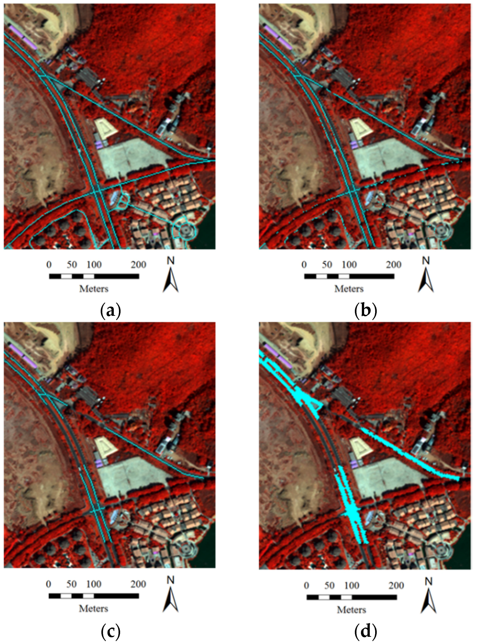
28]. In this research, the road networks are registered with the corresponding remote sensing images, and the training samples for roads can then be obtained. As shown in
Figure 1, accurate and reliable road sample detection consists of four steps: (a) registering the OSM road lines with the image; (b) removing the samples labeled by other classes; (c) removing short lines; and (d) sample extraction by buffering the road lines.
Figure 1.
Detection of road samples: (a) registering OSM road lines with the image; (b) removing samples labeled by other classes; (c) removing short lines; and (d) sample extraction by buffering road lines.
Figure 1.
Detection of road samples: (a) registering OSM road lines with the image; (b) removing samples labeled by other classes; (c) removing short lines; and (d) sample extraction by buffering road lines.
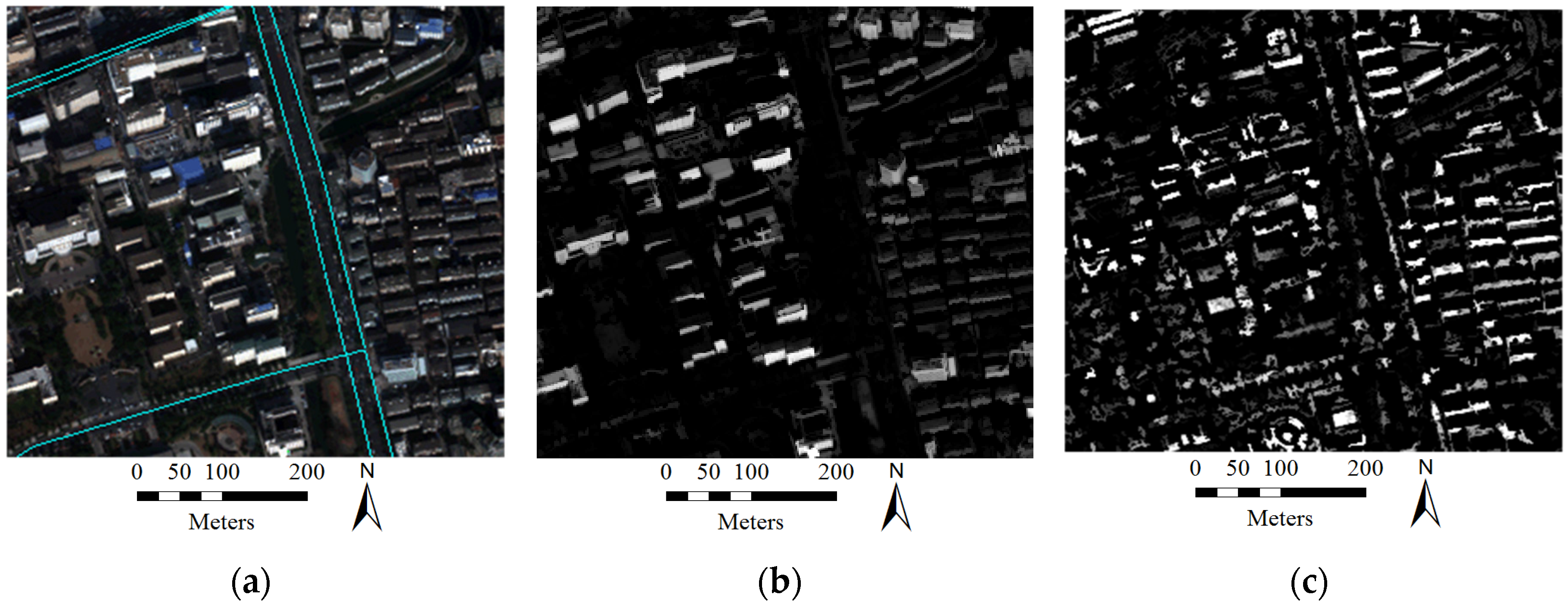
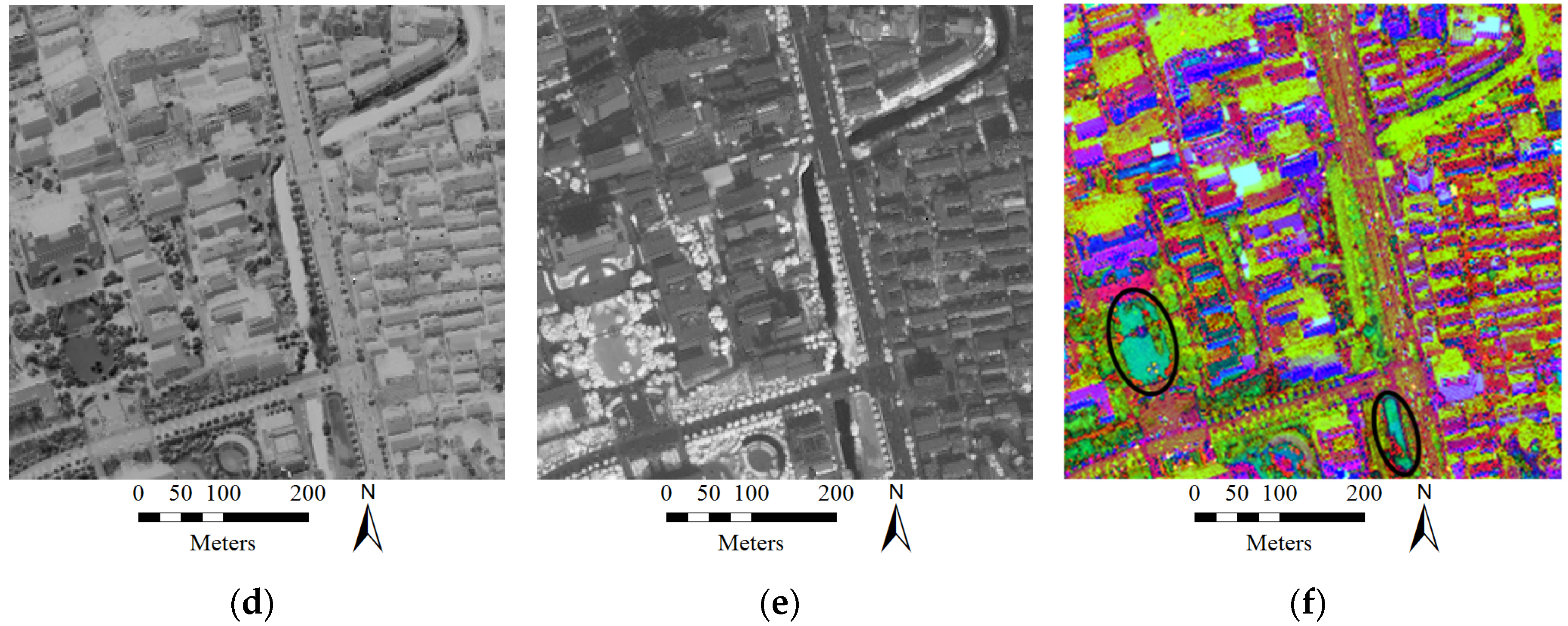
A graphic example of a WorldView-2 image is used to show the effectiveness of the information indexes, the HSV-based soil detection, as well as the OSM road lines for the automatic sample collection (
Figure 2). From the illustrations, it can be clearly seen that these information sources can provide effective descriptions of buildings, shadow, water, vegetation, soil, and roads. The visual results show that it is possible to automatically select candidate training samples. In particular, the soil components are highlighted as dark green in the HSV space, and can be detected as soil. However, it should be noted that there are overlaps between some similar classes, e.g., water and shadows. This suggests that the samples generated from the information sources cannot be directly used for classification, and refinement processing is needed.
Figure 2.
Multiple information sources, including (a) Roads from OSM; (b) MBI; (c) MSI; (d) NDWI; (e) NDVI; and (f) the HSV space, for selecting the initial sample set for roads, buildings, shadow, water, vegetation, and soil, respectively.
Figure 2.
Multiple information sources, including (a) Roads from OSM; (b) MBI; (c) MSI; (d) NDWI; (e) NDVI; and (f) the HSV space, for selecting the initial sample set for roads, buildings, shadow, water, vegetation, and soil, respectively.
3. Automatic Sample Selection
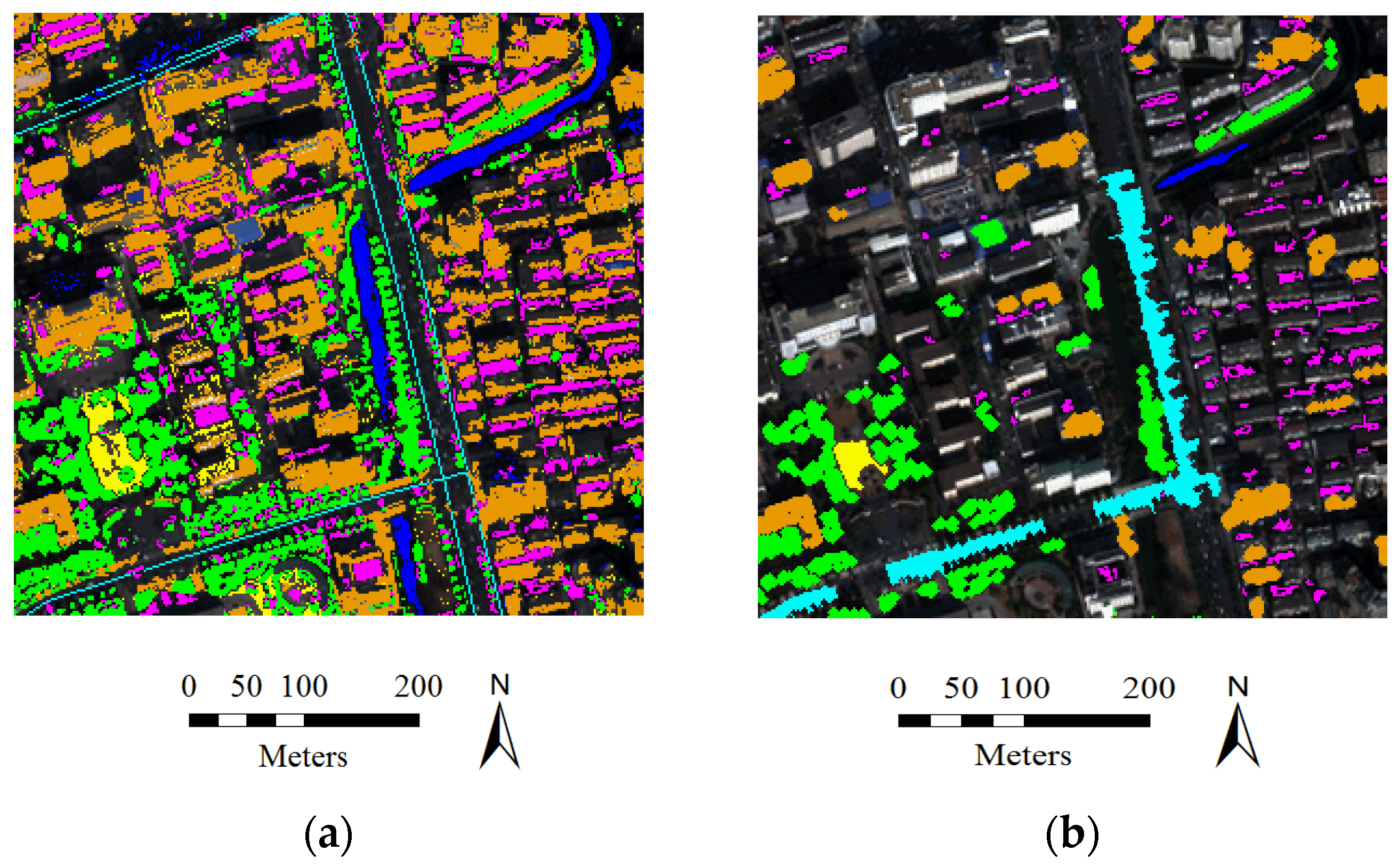
This section introduces the proposed method for the automatic selection of training samples for buildings, shadow, water, vegetation, roads and soil, as illustrated in
Figure 3, including the following steps.
- (1)
Select initial training samples of buildings, shadow, water, vegetation, soil, and roads, respectively, from the multiple information sources.
- (2)
Samples located at the border areas are likely to be mixed pixels, and, thus, it is difficult to automatically assign these pixels to a certain label. In order to avoid introducing incorrect training samples, these border samples are removed with an erosion operation.
- (3)
Manual sampling always prefers homogeneous areas and disregards outliers. Therefore, in this study, area thresholding is applied to the candidate samples, and the objects whose areas are smaller than a predefined value are removed.
- (4)
The obtained samples should be further refined, in order to guarantee the accuracy of the samples. Considering the fact that buildings and shadows are always spatially adjacent, the distance between the buildings and their neighboring shadows should be smaller than a threshold, which is used to remove unreliable buildings and shadows from the sample sets. Meanwhile, the road lines obtained from OSM are widened by several pixels, forming a series of buffer areas, where road samples can be picked out.
- (5)
Considering the difficulty and uncertainty in labelling samples in overlapping regions, the samples that are labeled as more than one class are removed.
Figure 3.
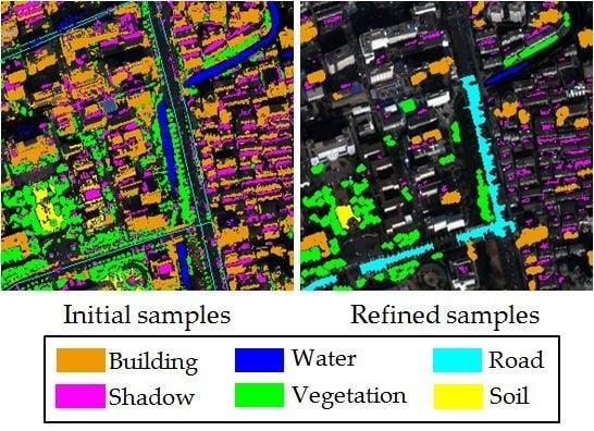
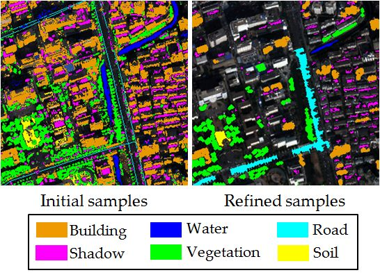
An example of a comparison between the initial samples derived from the multiple information sources and the samples refined by the proposed method (orange = buildings, magenta = shadow, blue = water, green = vegetation, cyan = roads, and yellow = soil). (a) Initial samples; (b) Refined samples.
Figure 3.
An example of a comparison between the initial samples derived from the multiple information sources and the samples refined by the proposed method (orange = buildings, magenta = shadow, blue = water, green = vegetation, cyan = roads, and yellow = soil). (a) Initial samples; (b) Refined samples.
The whole processing chain for the automatic sample selection is summarized in the following algorithm. Please note that the values of the parameters, mainly referring to the binarization threshold values for the multiple information indexes, and the area threshold values used to remove the small and heterogeneous points, can be conveniently determined and unified in all the test images. The suggested threshold values used in this study are not fixed, and can be appropriately tuned in different image scenes, but rather represent a first empirical approach.
| Algorithm: Automatic selection of training samples |
| 1: | Inputs: |
| 2: | Multiple information sources (MBI, MSI, NDWI, NDVI, HSV, OSM). |
| 3: | Manually selected thresholds (TB, TS, TW, TV). |
| 4: | Step1: Select initial training samples from the information sources. |
| 5: | Step2:
Erosion (SE=diamond, radius = 1) is used to remove samples from borders. |
| 6: | Step3: Minimal area (m2): ABuild = 160, AShadow = 20, AWater = 400, AVege = 200, and Asoil = 400. |
| 7: | Step4: Semantic processing: |
| 8: | (1) The distance between buildings and their adjacent shadows is smaller than 10 m (about |
| 9: | five pixels in this study). |
| 10: | (2) Road lines are widened for buffer areas. |
| 11: | Step5: Remove overlapping samples. |
In
Figure 3, the initial samples extracted by the multiple information sources and the samples refined by the proposed algorithm are compared, from which it can be seen that the pure samples for the land-cover classes are correctly labeled in an automatic manner.
5. Experiments and Results
A series of test images were used to validate the proposed method for the automatic selection of training samples. In the experiments, the proposed method was compared with the traditional method (i.e., manually collected samples), in order to verify the feasibility of the automatically selected samples.
5.1. Datasets and Parameters
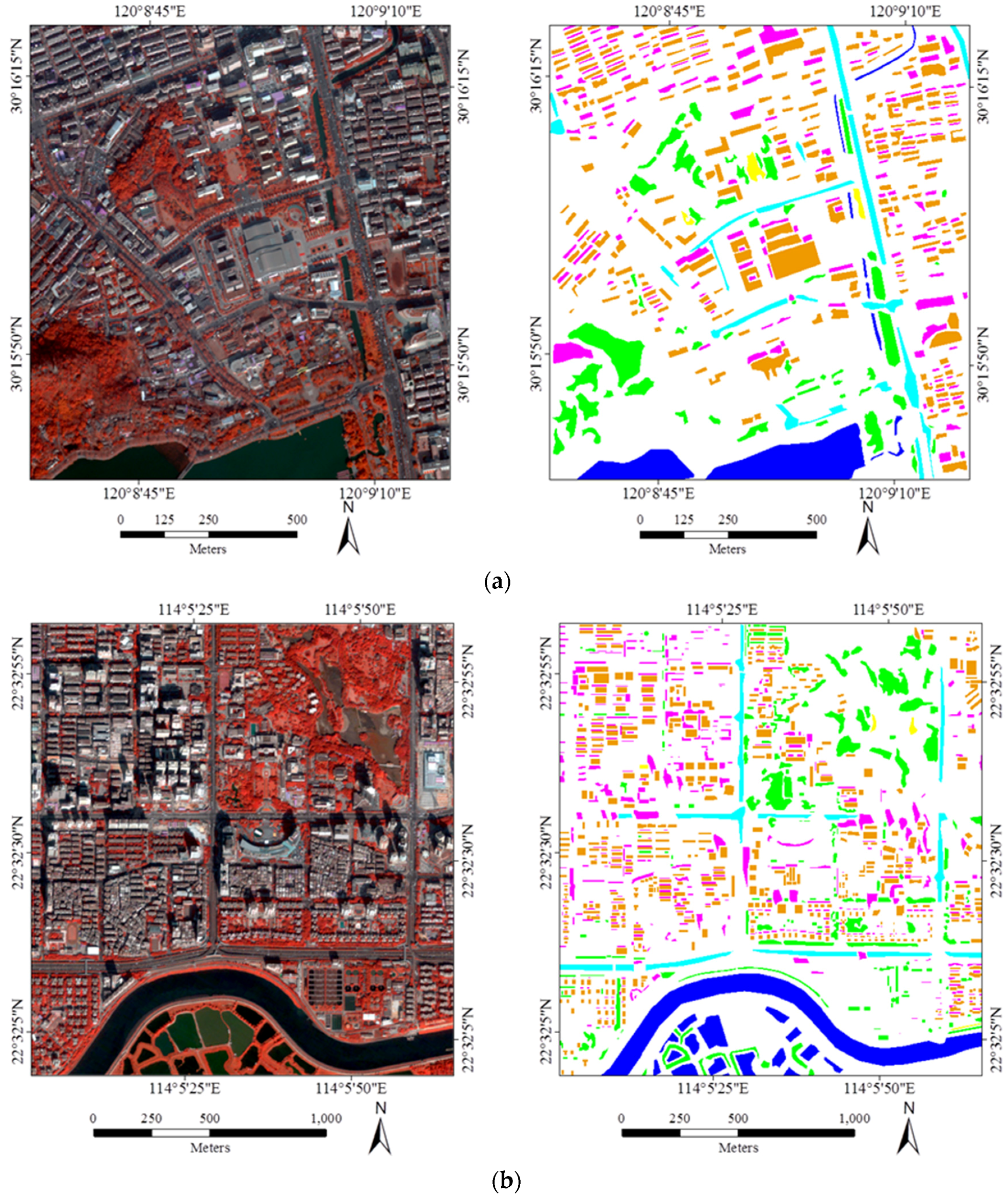
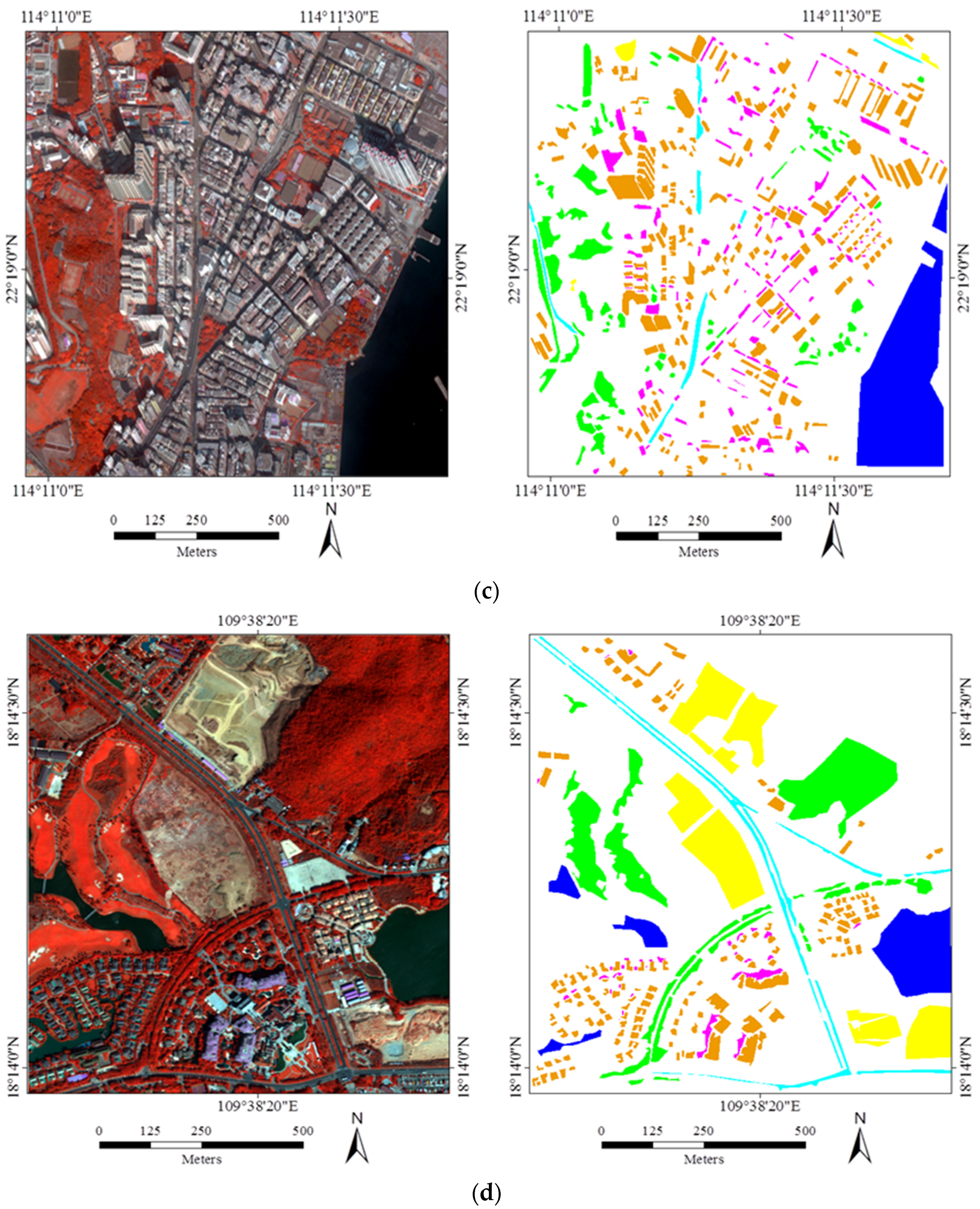
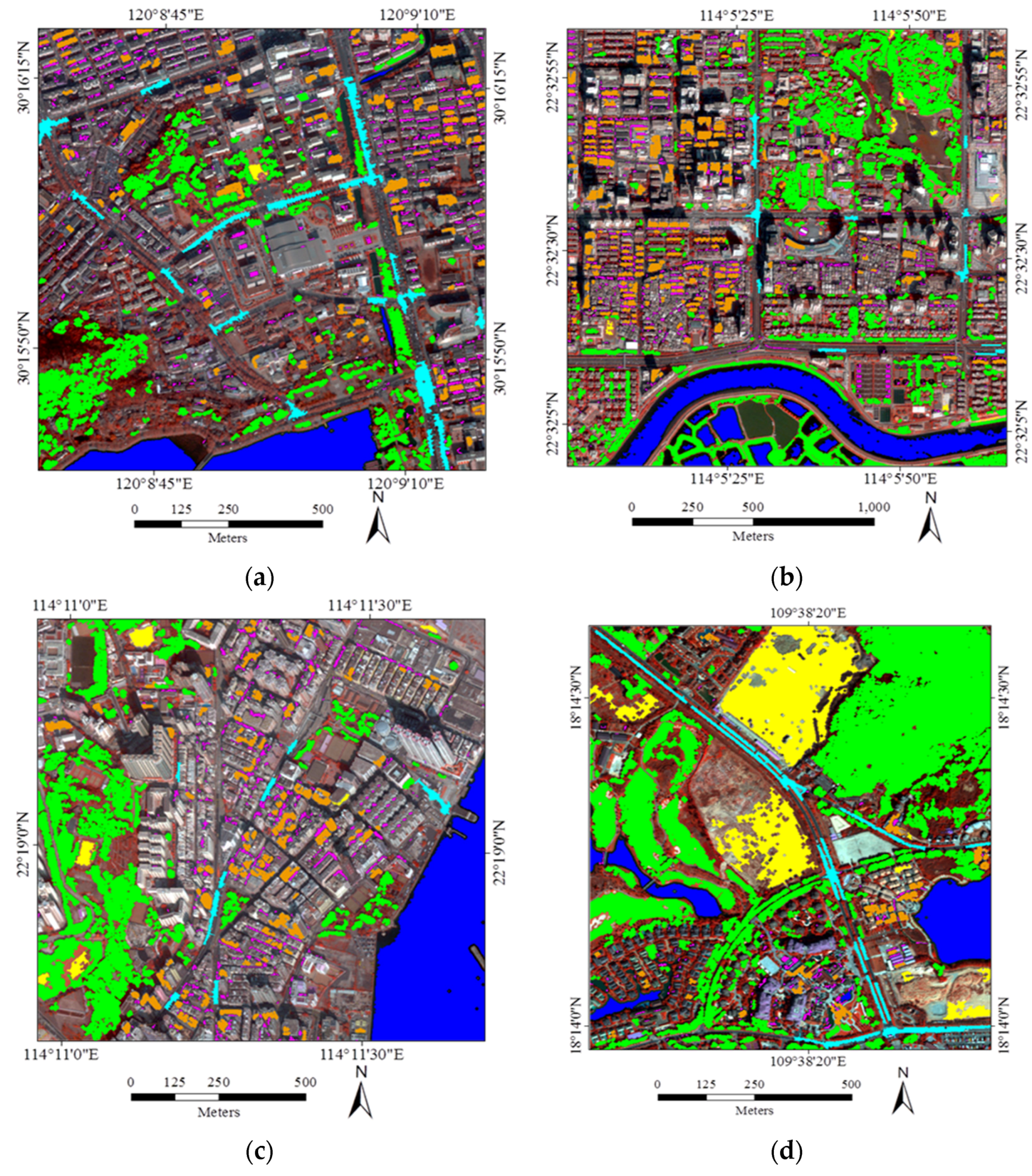
Figure 4 shows the four test datasets, as well as the manually selected samples (the ground truth). The study areas are located in Hangzhou, Shenzhen, Hong Kong, and Hainan, respectively, with a size of 640 × 594, 818 × 770, 646 × 640, and 600 × 520 in pixels, as well as a resolution of 2 m, 2.4 m, 2 m, and 2 m. These datasets were acquired by WorldView-2, GeoEye-1, WorldView-2, and WorldView-2, respectively, with eight, four, four, and eight spectral bands, respectively The study areas exhibit the characteristics of a set of typical urban landscapes in China, and mainly consist of six classes: buildings, shadow, water, vegetation, roads, and bare soil. The six classes can be automatically extracted by the proposed method, the effectiveness of which was tested in the experiments. For the manually collected samples, 40% of the labeled samples were randomly selected from the ground truth as the training sample set (named ROI in the following text), while the rest were used for the testing (
Table 1).
Figure 4.
The images (left) and ground truth (right) used in the experiments: (a) Hangzhou; (b) Shenzhen; (c) Hong Kong; and (d) Hainan (orange = buildings, magenta = shadow, blue = water, green = vegetation, cyan = roads, and yellow = soil).
Figure 4.
The images (left) and ground truth (right) used in the experiments: (a) Hangzhou; (b) Shenzhen; (c) Hong Kong; and (d) Hainan (orange = buildings, magenta = shadow, blue = water, green = vegetation, cyan = roads, and yellow = soil).
Table 1.
Numbers of training samples (ROI) and test samples, which were manually generated (in pixels).
Table 1.
Numbers of training samples (ROI) and test samples, which were manually generated (in pixels).
| Hangzhou | Shenzhen | Hong Kong | Hainan |
|---|
| ROI | Test | ROI | Test | ROI | Test | ROI | Test |
|---|
| Building | 13,004 | 19,507 | 16,598 | 24,897 | 12,388 | 18,583 | 4631 | 6947 |
| Shadow | 5742 | 8614 | 9774 | 14,661 | 3788 | 5682 | 570 | 857 |
| Water | 6186 | 9279 | 13,759 | 20,639 | 11,725 | 17,588 | 4,483 | 6726 |
| Vegetation | 7118 | 10,678 | 12,829 | 19,244 | 6042 | 9063 | 8601 | 12,902 |
| Road | 3784 | 5678 | 5185 | 7778 | 1264 | 1898 | 2142 | 3214 |
| Soil | 400 | 601 | 256 | 385 | 496 | 746 | 8875 | 13,314 |
The parameters of the linear structuring element (SE) for the MBI and the MSI, including the minimal value, maximal value, and the interval, {
Smin,
Smax, Δ
S,}, can be determined according to the spatial size of the buildings and the spatial resolution of the images used. These parameters were unified in this study as:
Smin = 8 m,
Smax = 70 m, and Δ
S = 2 m, respectively. In addition, the binarization threshold values for the information indexes were set according to the suggestions of our previous study [
25]. Please note that these thresholds can be simply and conveniently determined since we merely aim to choose pure and reliable samples for the further consideration.
For the SVM classifier, the radial basis function (RBF) kernel was selected, and the regularization parameter and kernel bandwidth was optimized by five-fold cross-validation. For the RF classifier, 500 trees were constructed. The MLP classifier was carried out with two hidden layers, and the number of neurons in each layer was also optimized by five-fold cross-validation.
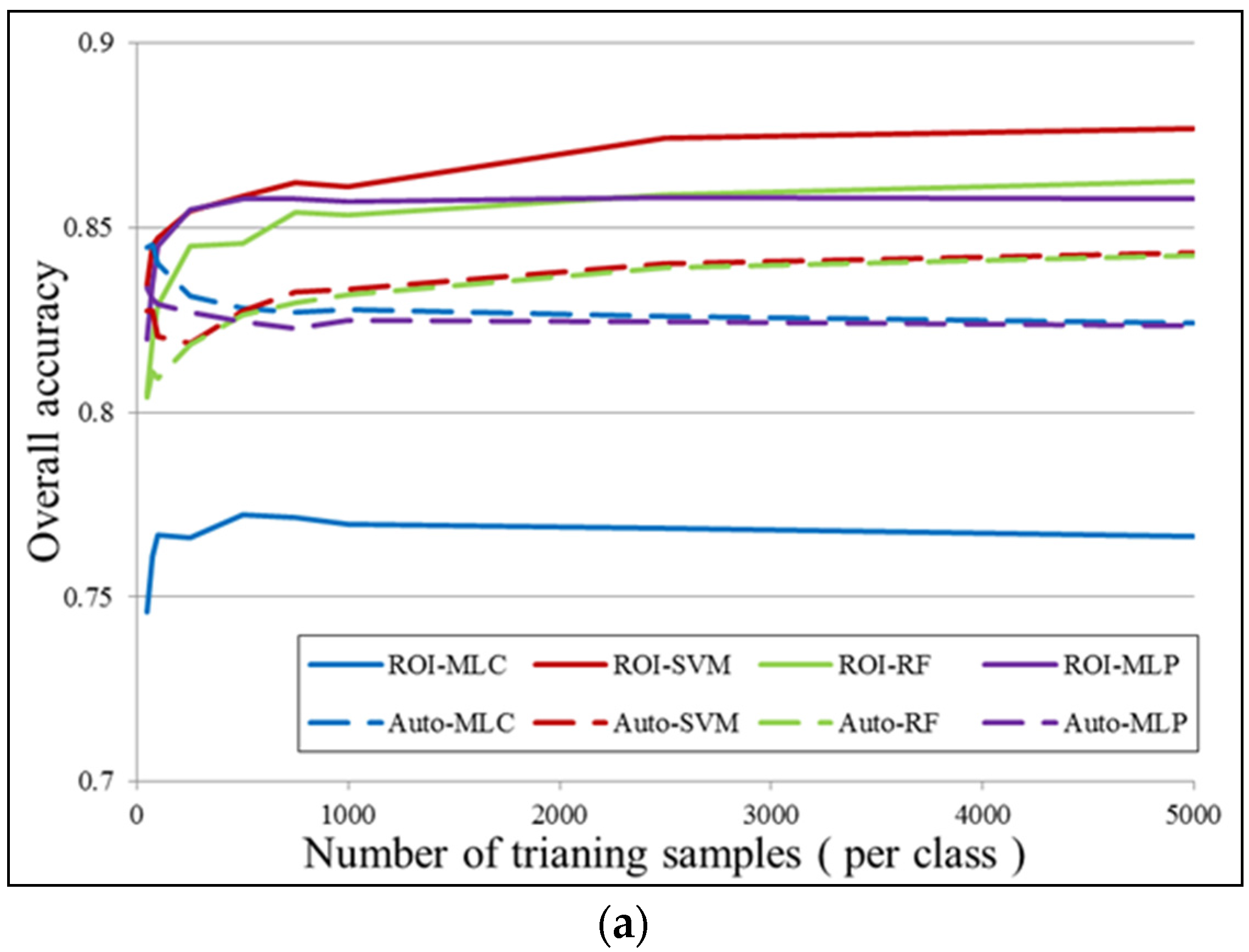
In the experiments, training with ROI or Auto means that the classification model was trained with manually labeled samples or automatically labeled samples, respectively. Each classification was conducted 10 times with different initial training samples that were randomly chosen from the candidate training sample set, and the average accuracies were recorded as the classification accuracy. For each classification experiment, 100 training samples per class were used for the training.
5.2. Results
The automatically selected training samples of the four datasets are displayed in
Figure 5, and their numbers are provided in
Table 2. It can be clearly observed that the automatically labeled samples are correct, pure, and representative, and are uniformly distributed in the whole image.
Figure 5.
Automatically labeled samples from the four datasets (orange = buildings, magenta = shadow, blue = water, green = vegetation, cyan = roads, and yellow = soil). (a) Hangzhou; (b) Shenzhen; (c) Hong Kong; (d) Hainan.
Figure 5.
Automatically labeled samples from the four datasets (orange = buildings, magenta = shadow, blue = water, green = vegetation, cyan = roads, and yellow = soil). (a) Hangzhou; (b) Shenzhen; (c) Hong Kong; (d) Hainan.
Table 2.
Numbers of automatically selected training samples (in pixels).
Table 2.
Numbers of automatically selected training samples (in pixels).
| Hangzhou | Shenzhen | Hong Kong | Hainan |
|---|
| Buildings | 10,686 | 24,177 | 12,287 | 3208 |
| Shadow | 7282 | 10,306 | 7126 | 1419 |
| Water | 17,418 | 34,307 | 41,569 | 13,572 |
| Vegetation | 29,801 | 83,425 | 44,571 | 85,022 |
| Roads | 8210 | 2938 | 2211 | 6170 |
| Soil | 269 | 852 | 2263 | 27,369 |
In general, from
Table 3, the Auto samples achieve satisfactory accuracies, which are close to the accuracies achieved by the ROI samples. In particular, for the Shenzhen and Hong Kong datasets, the classification results obtained by the Auto samples are very similar and comparable to the manually selected ones, for all the classifiers. With respect to the Hangzhou and Hainan datasets, the accuracy achieved by the proposed automatic sampling is also acceptable (80%~90%), although their accuracy scores are slightly lower than the ROI samples by an average of 4%~7%. Considering the fact that the proposed method is able to automatically select samples from the images, it can be stated that the method is effective, making it possible to avoid time-consuming manual sample selection.
Table 3.
The overall classification accuracies for the four datasets.
Table 3.
The overall classification accuracies for the four datasets.
| | MLC (%) | SVM (%) | RF (%) | MLP (%) |
|---|
| Hangzhou | Auto | 79.3 ± 1.7 | 80.4 ± 2.0 | 82.1 ± 1.2 | 82.6 ± 1.2 |
| ROI | 83.1 ± 1.7 | 85.6 ± 0.8 | 86.8 ± 0.9 | 86.4 ± 1.2 |
| Shenzhen | Auto | 81.8 ± 0.7 | 84.4 ± 1.0 | 84.0 ± 1.1 | 83.1 ± 2.0 |
| ROI | 82.8 ± 0.9 | 85.0 ± 0.9 | 85.1 ± 0.4 | 85.1 ± 0.8 |
| Hong Kong | Auto | 91.3 ± 0.6 | 90.2 ± 0.9 | 91.2 ± 0.5 | 91.0 ± 0.7 |
| ROI | 92.2 ± 0.7 | 90.3 ± 1.6 | 90.4 ± 1.1 | 91.1 ± 0.9 |
| Hainan | Auto | 88.3 ± 0.9 | 86.5 ± 1.9 | 85.4 ± 0.8 | 86.1 ± 0.9 |
| ROI | 94.1 ± 0.5 | 92.4 ± 0.7 | 90.2 ± 0.6 | 93.4 ± 0.5 |
When comparing the performances of the different classifiers with the Auto sampling, MLC achieves the highest accuracies in two test datasets (Hong Kong and Hainan). However, generally speaking, all the classifiers perform equally in the four test images, showing the robustness of the proposed automatic sampling method in different scenes.
5.3. Large-Size Image Testing
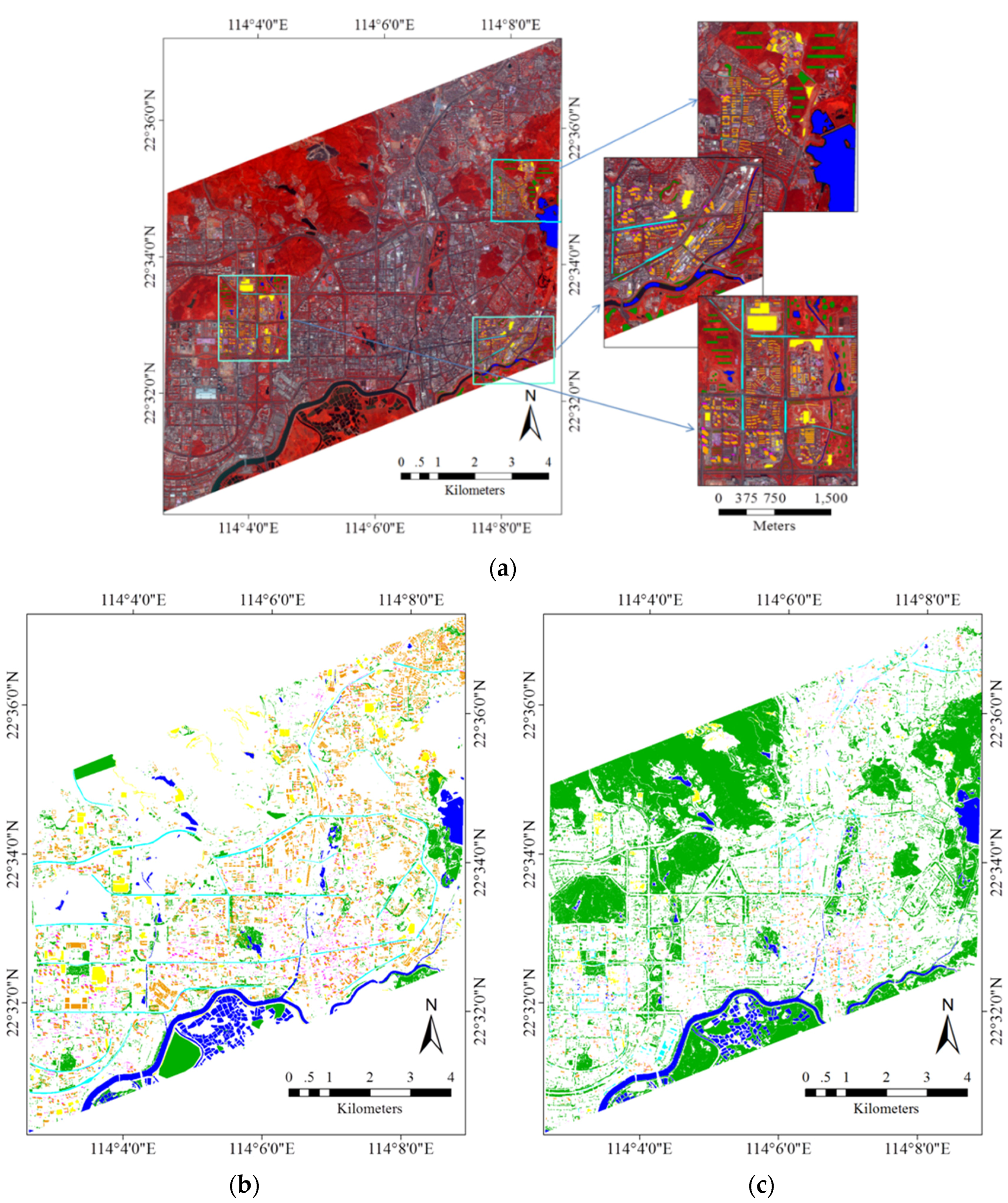
The previous experiments verified that the proposed automatic sampling strategy is able to achieve satisfactory classification results over the four urban images. We also tested the practicability of the automatic method by the use of a large-size image from the Shenzhen city center, which is China’s first and most successful Special Economic Zone. The dataset was acquired on 25 March 2012, by the WorldView-2 satellite, covering 92 km
2 with a 2-m spatial resolution, consisting of eight spectral bands. As shown in
Figure 6, the dataset (named WV-2 in the following text) covers the city center of Shenzhen, and three sub-regions are manually labeled as the source of the training samples (ROI). Please note that the whole image was manually labeled as the ground truth for testing, in order to guarantee the reliability of the experimental conclusions. The numbers of available samples for ROI, Auto, and test are provided in
Table 4. The parameters used in this experiment were the same as the previous ones.
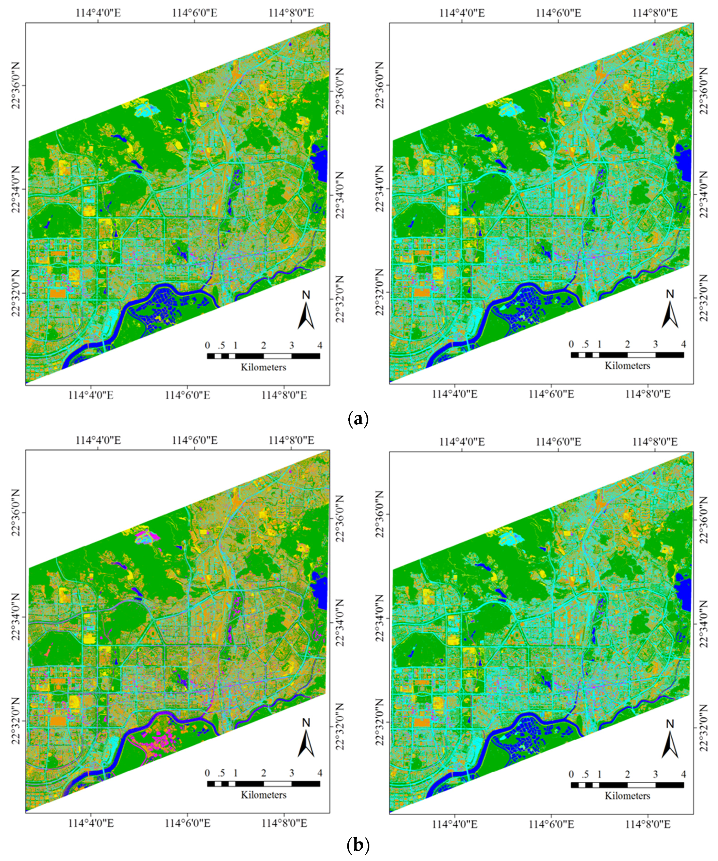
The classification results, including the quantitative accuracy scores and the classification maps, are shown in
Table 5 and
Figure 7, respectively. The experimental results convey the following observations:
In general, the classification accuracies obtained by the automatic sampling are very promising (80%~85%), which shows that it is fully possible to automatically classify large-size remote sensing images over urban areas.
By comparing the performances of the different classifiers, it can be seen that MLC achieves the highest accuracy for the Auto samples, while SVM and the MLP give the best results for the ROI samples.
It is interesting to see that in the case of MLC, the automatic sampling strategy significantly outperforms the manual sampling by 8% in the overall accuracy.
MLC performs better than the other classifiers with the automatic sampling. This phenomenon can be explained by: (1) the difference in the properties between the Auto and ROI samples; and (2) the difference in the decision rules between the classifiers.
Figure 6.
WV-2 Shenzhen image, as well as the three sub-regions as the source of the training sample set (ROI): ground truth of the whole image; automatically selected training sample set (Auto) (orange = buildings, magenta = shadow, blue = water, green = vegetation, cyan = roads, yellow = soil). (a) WV-2 urban image and training set; (b) Ground truth; (c) Automatic training set.
Table 4.
Numbers of samples for ROI, Auto, and test (in pixels).
Table 4.
Numbers of samples for ROI, Auto, and test (in pixels).
| Land Cover | ROI | Test | Auto |
|---|
| Buildings | 118,130 | 1,313,843 | 191,811 |
| Shadow | 14,446 | 185,650 | 76,723 |
| Water | 140,823 | 865,113 | 683,317 |
| Vegetation | 98,225 | 1,542,442 | 6,667,588 |
| Roads | 32,942 | 313,572 | 171,312 |
| Soil | 52,944 | 391,949 | 100,707 |
Table 5.
The overall accuracy of the classification for the WV-2 large-size image.
Table 5.
The overall accuracy of the classification for the WV-2 large-size image.
| Strategy | MLC (%) | SVM (%) | RF (%) | MLP (%) |
|---|
| Auto | 84.2 ± 1.0 | 81.8 ± 1.7 | 80.9 ± 1.2 | 82.5 ± 0.9 |
| ROI | 76.9 ± 2.2 | 84.0 ± 1.5 | 82.6 ± 1.2 | 84.9 ± 1.3 |
Figure 7.
Classification maps of the large-size WV-2 image with the Auto and ROI training samples. (a) Classification maps using the Auto training samples with MLC (left) and SVM (right); (b) Classification maps using the ROI training samples with MLC (left) and SVM (right).
Figure 7.
Classification maps of the large-size WV-2 image with the Auto and ROI training samples. (a) Classification maps using the Auto training samples with MLC (left) and SVM (right); (b) Classification maps using the ROI training samples with MLC (left) and SVM (right).
It should be noted that the Auto samples are purer than ROI, since the automatic selection prefers homogeneous and reliable samples in order to avoid errors and uncertainties. Specifically, as described in Algorithm 1, boundary pixels which are uncertain and mixed have been removed, and the area thresholding further reduces the isolated and heterogeneous pixels.
The four classifiers considered in this study can be separated into parametric classifiers (MLC), and non-parametric classifiers (SVM, RF, and MLP). The principle of MLC is to construct the distributions for different classes, but the non-parametric methods tend to define the classification decision boundaries between different land-cover classes. Consequently, pure samples are more appropriate for MLC, but an effective sampling for the non-parametric classifiers is highly reliant on the samples near the decision boundaries so that they can be used to separate the different classes.
7. Conclusions and Future Scope
In this paper, a novel method for automatic sample selection and labelling for image classification in urban areas is proposed. The training sample sets are obtained from multiple information sources, such as soil from the HSV color space, roads from OSM, and automatic information indexes referring to buildings, shadow, vegetation, and water. A series of processing steps are further used to refine the samples that are initially chosen, e.g., removing overlaps, removing borders, and semantic filtering.
The experiments with four test datasets showed that the proposed automatic training sample labelling method (Auto) is able to achieve satisfactory classification accuracies, which are very close to the results obtained by the manually selected samples (ROI), with four commonly used classifiers. Furthermore, the experiments with a large-size image (WorldView-2 image from Shenzhen city, 92 km
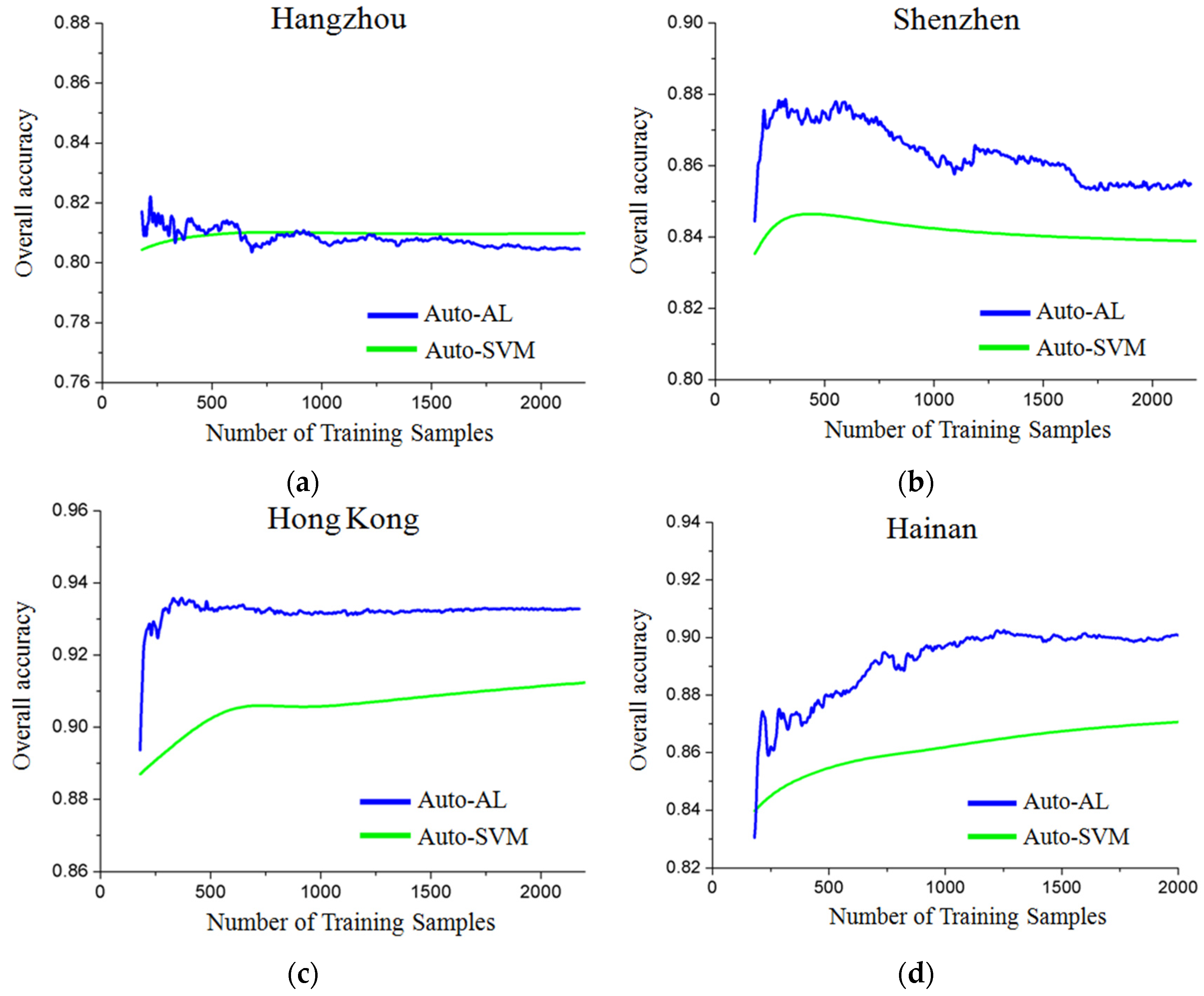
2) showed that the proposed method is able to achieve automatic image classification with a promising accuracy (84%). It was also found that the automatic sampling strategy is more suitable for maximum likelihood classification (MLC), which aims to describe the probabilistic distribution of each land-cover class. In particular, in the experiments, active learning [
40] was jointly used with the proposed Auto sampling method, in order to select the most informative samples from the automatically labeled samples. The results were interesting and promising, as active learning could further improve the classification accuracies by about 2%~4% in most of the test sets.
The significance of this study lies in the fact that it has showed that automatic sample selection and labelling from remote sensing images is feasible and can achieve promising results. Our future research will address the mixing of manually and automatically selected samples. In this way, the decision boundaries generated by the Auto method could be further enhanced by adding new samples and removing wrong ones. It will also be possible to evaluate and compare the importance of manual and automatic samples for classification. In addition, the samples used for the accuracy assessment will be generated randomly, in order to avoid any bias in the results [
41].


