Article

A Hybrid Kernel-Based Change Detection Method for Remotely Sensed Data in a Similarity Space

by
Reza Shah-Hosseini
1,
Saeid Homayouni
2 and
Abdolreza Safari
1,*
1
University College of Engineering, School of Surveying and Geospatial Engineering, University of Tehran, Tehran 11155-4563, Iran
2
Department of Geography, University of Ottawa, Ottawa, ON K1N 6N5, Canada
*
Author to whom correspondence should be addressed.
Remote Sens. 2015, 7(10), 12829-12858; https://doi.org/10.3390/rs71012829
Submission received: 31 May 2015 / Revised: 4 September 2015 / Accepted: 17 September 2015 / Published: 30 September 2015

Abstract

:
Detection of damages caused by natural disasters is a delicate and difficult task due to the time constraints imposed by emergency situations. Therefore, an automatic Change Detection (CD) algorithm, with less user interaction, is always very interesting and helpful. So far, there is no existing CD approach that is optimal and applicable in the case of (a) labeled samples not existing in the study area; (b) multi-temporal images being corrupted by either noise or non-normalized radiometric differences; (c) difference images having overlapped change and no-change classes that are non-linearly separable from each other. Also, a low degree of automation is not optimal for real-time CD applications and also one-dimensional representations of classical CD methods hide the useful information in multi-temporal images. In order to resolve these problems, two automatic kernel-based CD algorithms (KCD) were proposed based on kernel clustering and support vector data description (SVDD) algorithms in high dimensional Hilbert space. In this paper (a( a new similarity space was proposed in order to increase the separation between change and no-change classes, and also to decrease the processing time, (b) three kernel-based approaches were proposed for transferring the multi-temporal images from spectral space into high dimensional Hilbert space, (c) automatic approach was proposed to extract the precise labeled samples; (d) kernel parameter was selected automatically by optimizing an improved cost function and (e) initial value of the kernel parameter was estimated by a statistical method based on the L2-norm distance. Two different datasets including Quickbird and Landsat TM/ETM+ imageries were used for the accuracy of analysis of proposed methods. The comparative analysis showed the accuracy improvements of kernel clustering based CD and SVDD based CD methods with respect to the conventional CD techniques such as Minimum Noise Fraction, Independent Component Analysis, Spectral Angle Mapper, Simple Image differencing and Image Rationing, and also the computational cost analysis showed that implementation of the proposed CD method in similarity space decreases the processing runtime.

Graphical Abstract

1. Introduction

The analysis of multi-temporal Earth observations is essential for change detection (CD) applications [1]. This process is for identifying the differences in spatial, spectral, and radiometric states of phenomenon by observing it at different times [2]. CD is a useful technique for various applications such as land-cover/land-use change analysis, assessment of deforestation, damage assessment, disaster monitoring, and other environmental changes [1]. For this purpose, several CD methods have been developed for analyzing and detecting the changed areas from multi-temporal images [3,4]. It has been generally agreed that change detection is a complicated and integrated process. So far, there is no existing approach that is optimal and applicable in the case of (a) labeled samples not existing in the study area; (b) existence of different environmental factors such as atmospheric and light conditions in multi-temporal images; (c) multi-temporal images corrupted by either noise or radiometric differences that cannot be normalized and (d) difference images have overlapped change and no-change classes that are non-linearly separable from each other. Furthermore, for the time being, the degree of automation is far too low for real-time CD applications. Hence this paper aims to resolve the issues mentioned above.
Change detection methods are divided into six categories in the literature: (a) Images algebra (b) Change Vector Analysis (CVA); (c) Image transformation; (d) Post-classification comparison (e) Direct classification; and (f) Hybrid CD [5,6,7]. In images algebra method, mathematical operations such as subtraction or division applied to multi-temporal imagery; providing the difference or ratio images [8,9]. In CVA approach by computing the difference vectors between multi-temporal images, providing both the magnitude and direction of the change [10,11]. In both images algebra and CVA change detection methods digital values of difference pixels or magnitude pixels are numerically compared with a pre-defined threshold to generate the change map. These two methods are non-automatic and ineffective, because determining the appropriate threshold becomes a difficult and time-consuming task and can fail in real time applications such as disaster management [12,13]. However, image transformation methods are based on mathematical transformation to highlight the variance between images and provide a well-designed approach to handle high dimensional data. There is no defined thematic meaning the output of this method and changed area may be difficult to locate and interpret [14].
Post-classification comparison technique is based on the comparison of multiple classification maps to detect the class transitions between multi-temporal images [15]. In direct classification method, multi-temporal images are stacked together and then classified directly in order to detect the land cover transition [16]. In both classification based methods, labeled samples are essential for training the supervised classifiers. Nevertheless, preparing of samples for training the classifiers can be a difficult task, especially for a time series of images. All classifiers are, in general, sensitive to the noise of pixels in multi-temporal images. On the other hand, multi-temporal classification methods are based on linear representations, and do not consider the non-linear cross-information among the pixels in different time [17,18]. As a result, the classifier trained with samples coming from different distributions due to differences in atmospheric and light conditions. So, classification errors in each of the input maps are directly transformed to the generated change map. Therefore, they can be inefficient for images corrupted by either noise or radiometric differences that cannot be normalized or, in the case of multi-temporal images, which have spectrally overlapped classes [1,19,20].
To address these problems, several strategies have been presented and the approaches considered knowledgeable threshold-based image differencing or ratioing. Bruzzone and Prieto [21] propose two unsupervised CD techniques based on the Bayes theorem. The first method is based on an automatic threshold selection that minimizes the overall change detection error probability. The second method analyzes the difference image by considering the spatial-contextual information included in the neighborhood of each pixel. The accuracy of the analysis of proposed methods was carried out on two different data sets including Landsat 5 TM sensor and the synthetic data. The experimental results certified the effectiveness of both proposed methods. Molina et al. [22] suggested a multisource CD approach for multi resolution data sets. After extraction of various change indices, different thresholding algorithms were applied to these indices. The indices are then integrated into a change detection multisource fusion procedure, for generating a final CD map. This method has been applied to airborne and spaceborne optical imageries with different spectral and spatial resolutions. The proposed CD algorithm has proven to be efficient with respect to using various spatial resolutions of sensors. In some studies, the methods based on a similarity measure extraction and determining a proper threshold are used for automatic change detection. Inglada and Mercier [23] presented a new similarity measure for automatic change detection in multi-temporal SAR images. Tests on the simulated and real data showed that this detector performs better than all the other methods. Mercier et al. [24] showed how to obtain a binary change map from the similarity measures of the local statistics of images before and after a disaster. The decision process is achieved by the use of a Support Vector Machines (SVM) approach in which a stochastic kernel has been defined. The results have shown the efficiency of the methods since it yields an appropriate binary change map for multi-sensor change detection. However, this was demonstrated to be inefficient based on the reasons stated earlier in the case real-time CD problems.
On the other hand, change detection can be viewed as a particular case of the multi-temporal image classification problem. Pajares [25] proposed an automatic method based on the Hopfield Neural Network (HNN) for image change detection. Each pixel in the difference image is a node in the HNN. This method, unlike classical methods [21,26], uses the performance of contextual and self-data information by integrating the data and contextual information under the form of an energy function. The self-data information minimizes the errors derived from incorrect decisions taken by the neighbors of a pixel. The experimental results showed that the proposed method has proven to be robust against noise as compared with the classical methods. Nevertheless, the main disadvantage of the HNN method originates from its high time consuming process. This approach, however, inherits all the aforementioned problems of the classification-based CD scenario.
It is only recently that authors have turned to kernel-based CD methods for change detection applications [12]. Guorui et al. [27] proposed a Distance-based Kernel Change Detection algorithm (DKCD). The multi-temporal images are mapped into a feature space via nonlinear mapping. Then, a simple distance measure between two feature vectors defined in feature space. Their results proved a reliable performance with respect to the speed and accuracy of change detection mapping. Camps-Valls et al. [28] present a kernel-based method based on Support Vector Domain Description (SVDD) classifier for change detection of remote sensing images. Good performance of the proposed method illustrates the generality of the algorithms. Volpi et al. [17] have presented an unsupervised clustering method based on an SVM classifier to find the changes in multi-temporal co-registered images. Two change detection schemes were adapted for very high resolution optical imagery (VHR): multi-date classification and difference image analysis. Experiments on VHR images proved the reliability of the proposed approach. In kernel-based methodologies kernel-based discrimination amongst the classes of interest can be enhanced by using the nonlinear decision function and better results will be achieved. These types of decision functions are locally linear, but in general have a complex shape that is not equivalent to a line in 2D or a hyperplane in higher dimensions [29].
The main idea of kernel methods is based on the fact that the nonlinear decision function can be obtained by running a linear algorithm in a higher dimensional reproducing kernel Hilbert space (RKHS). In classification of multi-temporal remotely-sensed data, a linear decision function is clearly not sophisticated. The traditional classification approaches solve these problems by using more sophisticated distributions in modelling the optimal Bayes classifier. But, these methods are computationally more expensive. An efficient method in this field is the kernel concept which was originally applied in support vector machines technique. The linear decision function in the kernel space corresponds to a forceful nonlinear decision function in the spectral space [12]. The mapping to that space is implicitly defined by kernel functions replacing dot products in the original formulation in spectral space [2]. In the change detection problem, these kernel methods allow modeling the nonlinear nature of the change [30]. However, none of these methods considers the cross relations between multi-temporal images in the classifier. Also, these non-automatic kernel-based methods require labeled samples for training a classifier, and as a result, they are still inefficient in real-time CD applications.
In Hybrid CD method, multiple comparison methods within a framework were used. The most commonly used strategy is a combination of images algebra and direct classification methods for the detection and classifying the changes [31,32]. This strategy was used in this paper for developing the proposed CD method. Due to attending to the previously identified problems, in this paper, a hybrid kernel-based change detection method was proposed in a similarity space which has demonstrated good results in image change detection problems with few labeled training samples in high dimensional spaces. This proposed method used all single and cross information between the multi-temporal images bands and presents a nonlinear solution in Hilbert space for the change detection problem. This leads to a strong decrease in the false alarm rate (classifying a background pixel as a change class), and a slight accuracy improvement in the generated change map. Meanwhile, the initialization of proposed algorithm was addressed automatically by finding a threshold on change vector magnitude distribution.
In parallel with the proposed kernel-based CD algorithm, an SVDD-based change detection method was presented and analyzed. These methods were applied on Landsat TM/ETM+ and Quickbird multi-spectral imageries for mapping and estimating the deforestation and damaged areas caused by human activity and natural disasters, respectively. This proposed kernel-based CD method uses three approaches for mapping the data from the spectral space into higher dimensional Hilbert space. The first is based on the difference image in the spectral space, which is named as DFSS (Differential in Spectral Space). In the second approach, to provide the most discriminative information, a mapping function is developed to compute the difference image in Hilbert space, i.e., Differential in Hilbert Space (DFHS). Finally, in the third approach, multi-temporal images are stacked together in spectral space and then transformed into Hilbert space, namely as Heaped in Spectral Space (Heap-SPC). In Hilbert space, the complicated and nonlinear relationship between the data could be modeled linearly. By using a similarity space, the separation between change and no-change classes increased and time of the process decreased. In a particular case, the multi-temporal data are transformed into a Spectral Distance-Angle-Correlation-Spectral Value (SDACV) space [33]. In order to determine the threshold and extract the precise training samples, a method based on integration of a Change Vector Analysis (CVA) technique and kernel-based K-means clustering algorithm was proposed. On the other hand, proper kernel parameters of the proposed kernel-based methods were determined by using a developed cost function based on geometric and spectral similarity criteria. This precise training set was used for training the Kernel-based Minimum Distance (KMD) and the Support Vector Data Description (SVDD) classifiers.

2. Methodology

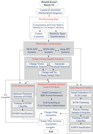
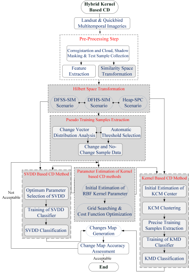
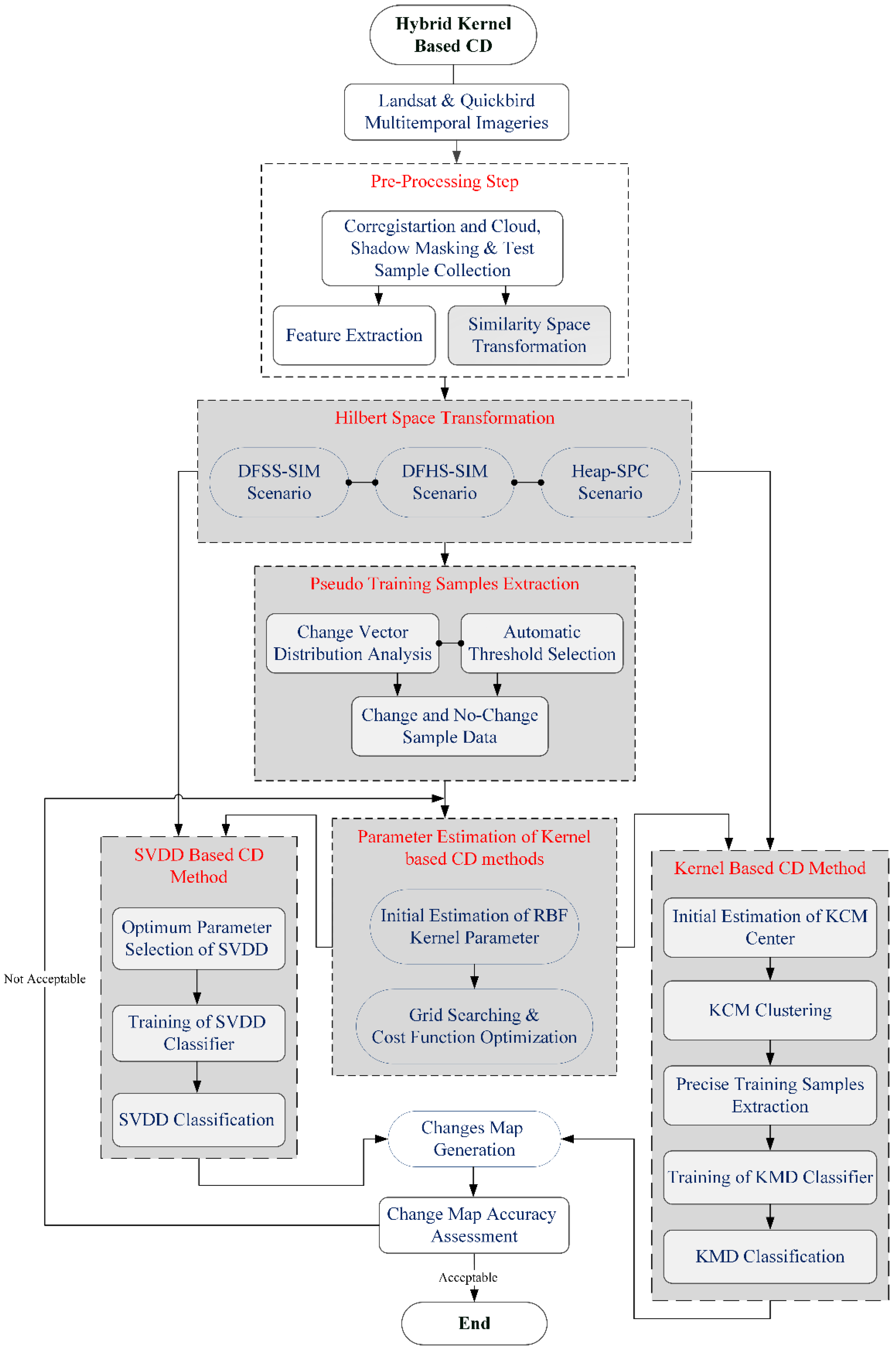
2.1. Proposed Framework

Proposed kernel-based CD framework refers to several proposed stages, including: (a) Pre-processing step; (b) similarity space and Hilbert space transformations; (c) pseudo training samples extraction; (d) parameter estimation of kernel-based CD methods; (e) kernel-based CD method and (f) SVDD based CD method. The flowchart of proposed method for automatic detection of changes is presented in Figure 1. As it can be seen, our focus in this paper illustrated as highlighted stages in block diagram.
In the first step of implementation, the geometric and the radiometric preprocessing are performed on the multi-temporal images. Then the multi-temporal images are co-registered manually to each other. Cloudiness of the study area in the Quickbird dataset is symmetrically masked. In the second step, the multi-temporal images are transformed into a similarity space. To this end, a reference vector is needed to measure the similarity of all the pixels in the multi-temporal images. Since the objective of proposed algorithm is mapping the changes, the reference vector of change class was used. After extracting the precise training data, the mean of precise changed training samples was calculated in order to achieve the reference change vector. Then, using the Equations (13)–(16) and the reference vector from the previous step, all pixels of the image are transformed into the similarity space. In this paper, the multi-spectral data are transformed to similarity spaces using Spectral Distance-Angle-Correlation-Spectral Value (SDACV) features [34].
Figure 1. Block diagram of proposed hybrid kernel-based change detection algorithm.
Remotesensing 07 12829 g001
In the next step, for transferring the multi-temporal images into Hilbert space, three approaches between the corresponding bands were performed in Hilbert space. The first approach accounts for the difference image in the similarity space, which is named as DFSS-SIM (Differential in Similarity Space). In this method, the multi-temporal images are first transferred into similarity space and then subtracted in a pixel-by-pixel method to obtain the difference image, i.e., D R d . The difference pixels are then mapped to the Hilbert space as φ(x) = φ(xd), resulting in the kernel function K(xid, xjd) = φ(xid), φ(xjd). In the second approach, to provide the most discriminative information, a mapping function is developed to compute the difference image in Hilbert space which is named DFHS. For a given pixel, the RKHS feature map φ(.) corresponding to the difference pixel can be defined as: φ ( x i ) = Η ( t 2 ) φ ( x i ( t 2 ) ) Η ( t 1 ) φ ( x i ( t 1 ) ) .   Expanding the dot product and exploiting Mercer’s conditions, the corresponding kernel function is obtained [12,35]:
K ( x i , x j ) = φ ( x i ) , φ ( x j ) = K ( x i ( t 2 ) , x j ( t 2 ) ) + K ( x i ( t 1 ) , x j ( t 1 ) ) K ( x i ( t 2 ) , x j ( t 1 ) ) K ( x i ( t 1 ) , x j ( t 2 ) )
In the third approach, before and after images are stacked together before and after in spectral space and then transformed into Hilbert space, which is named as Heap-SPC. The main issue of the automatic change detection algorithms is to find a proper initialization allowing the method to converge to a global minimum. For this reason, in the next step, by analyzing the components of a change vector and setting an appropriate threshold, pseudo training samples are created for the change and no-change classes. These sample data are being used for determining the imprecise initial set of kernel K-means clustering parameters and training the SVDD-based change detection method [17]. Then, the precise training samples and kernel K-means parameters are automatically estimated by optimizing a cost function with the nature of geometrical and spectral similarity in kernel space. These samples are used as training data for training of KMD classifiers. After the training stage of KMD classifier and SVDD-based change detection method and optimization of its parameters, each pixel entered into a proposed methods and the class of each pixel is determined. The output of this step is the change map.
In DFHS approach, the difference kernel needs the estimation of the corresponding kernel parameters, e.g., two bandwidths when using two RBF kernels corresponding to two kernels in Equation (17). In this paper, a search among two parameters θ = {σsingle, σcross} with respect to K ( x i t i , x j t i ) and K ( x i t i , x j t j ) is performed [35]. To solve this problem, a new method to estimate the initial value of the RBF kernel parameter in the change detection problem was employed. This method is based on a statistical technique and uses the L2 distance norm. In this new method, in the first step, two sets of spectral vectors within the first image are elected randomly. In the next step, Euclidean distance between two spectral vectors in the first image is computed and the median of this distance is selected [33]. The same process is performed for the second image. Finally, the average of the two distances, obtained from multi-temporal images, is considered as the initial estimation of RBF kernel parameter. In the next step, a change interval is considered with respect to the initial value, so that this value is in the center of a change interval. These ranges can be used in the grid search method to select the precise RBF kernel parameter [33,36]. This new method leads to a faster convergence of grid-searching technique for selecting the global optimum RBF kernel parameter.

2.2. Thresholding Scheme

The main issue of proposed kernel-based CD algorithms is to find a proper threshold allowing the method to extract two pseudo training samples with high probability rate, belonging to change and no-change classes. In order to estimate the change and no-change class distributions, the magnitude of spectral change vector was calculated. This distribution can be seen as a mixture of two Gaussian models regarding change and no-change pixels. In the next step, by analyzing the magnitude of a change vector and setting an appropriate threshold, the pseudo training samples were created for change and no-change classes [17]. In this paper, the proper threshold was determined by fitting a Gaussian function to change the vector magnitude’s distribution of multi-temporal images. The mean and variance values of Gaussian function were estimated and used as a threshold. The extracted pseudo training samples were then used for determining the imprecise initial set of kernel clustering algorithm parameters such as cluster center.

2.3. Kernel K-Means Clustering

The kernel K-means clustering algorithm (KKMC) rewriting the linear K-means in RKHS (Reproducing Kernel Hilbert Space) by means of mapping functions φ(.). The mapping to that space is implicitly defined by the kernel functions replacing the dot products in the original formulation, which only needs input samples in their spectral space. Since the K-means formulation can be expressed solely in the terms of dot products, kernel functions can replace these expressions. This helps the value of the dot product to return directly to the RKHS [35]. Let X = {a1, a2, a3, ..., an} be the set of data points and “c” the number of clusters. In the first step “c” cluster centers are randomly initialized. The kernel k-means algorithm is formulated as the minimization of the sum of the squares of distances between mapped samples and their mean:
d ( φ ( x ) , μ ) = q = 1 K i ϵ π q φ ( x i ) μ q 2
where μq denotes the mean of the cluster q and φ ( x ) π q is the mapped samples in the RKHS. By replacing μ q = n q 1 j π q φ ( x j ) and applying the kernel substitution, Equation (2) becomes:
d ( φ ( x ) , μ ) = K ( x i , x i ) 2 n q j ϵ π q K ( x i , x j ) + 1 n q 2 j , l ϵ π q K ( x j , x l )
where nq is the number of samples is assigned to the cluster q. The position of cluster centers, are approximated by considering the closest samples to the center x c = arg min x i d ( φ ( x i ) , μ q ) . After determining the clustering parameters, each data point assign to that cluster center whose distance is minimum [37].

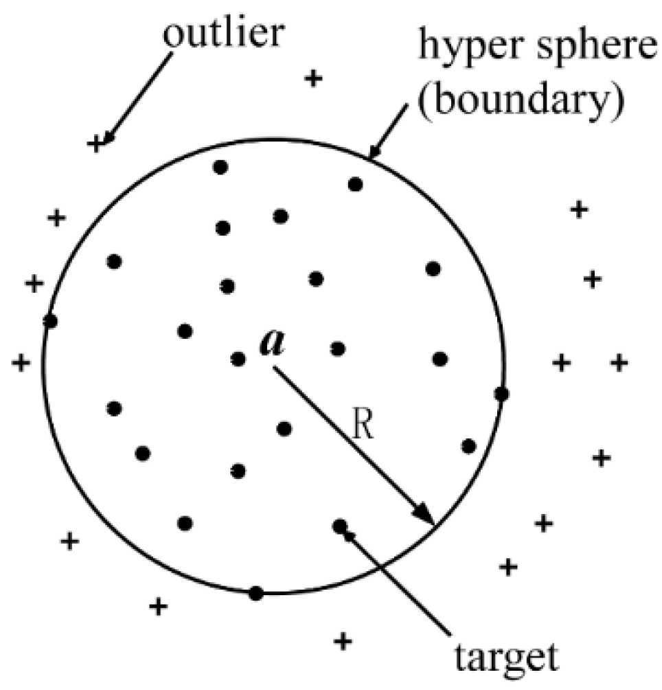
2.4. Support Vector Data Description

In parallel with the proposed algorithm, another method based on Support Vector Data Description (SVDD) was presented and analyzed. After extracting the pseudo training samples of change and no-change regions, these samples are used to train the SVDD classifier. Now assuming a dataset { x i } i = 1 N belongs to a given class of interest. The objective here is to find a hyper-sphere in a high dimensional Hilbert space of radius R > 0 and center a, with a minimum volume containing most of these data points [28,38] (See Figure 2).
Figure 2. Schematic diagram of support vector data description. The hyper-sphere is described by the center a and radius R [39].
Remotesensing 07 12829 g002
Therefore one has to minimize R2 constrained to φ ( x i ) a 2 R 2 , i = 1 , ... , n . However, since the training distribution may contain outliers; one introduces a set of slack variables ξ i > 0 and the problem then becomes [28]:
min R , a { R 2 + C i ξ i }
Constrained to
φ ( x i ) a 2 R 2 + ξ i , ξ i 0 , i = 1 , ... , n
Where the parameter C controls the trade-off between the volume of the hyper-sphere and the acceptable errors (penalty parameter).The dual functional now becomes [28,38]:
max α i { i α i φ ( x i ) , φ ( x i ) i , j α i α j φ ( x i ) , φ ( x j ) }
Subject again to 0 α i C this constitutes a quadratic programming problem that yields a set of α i fulfilling that (i) if φ ( x i ) a 2 < R 2 then α i = 0 (ii) if φ ( x i ) a 2 = R 2 the 0 < α i < C , and (iii) if φ ( x i ) a 2 > R 2 then α i = C As a result, Support Vectors (SV) are those satisfying α i > 0 , while samples whose associated α i = C are considered outliers. An equivalent formulation was proposed, in which one places a hyper-plane that separates the data from the origin with maximum margin (Figure 2). In this case the problem reduces to [28,38]:
min w , ρ , ξ { 1 2 w 2 ρ + 1 υ η i ξ i } i = 1 , ... , n
Constrained to ξi ≥ 0 and where ν ∈ (0,1] is a regularization parameter (C) controlling the trade-off between accepting data into the class and having w small. Introducing again Lagrange multipliers we reach the (equivalent) dual problem [28,38]:
min α i { 1 2 i , j α i α j φ ( x i ) , φ ( x j ) } = min α { 1 2 i , j α i α j K ( x i , x j ) }
Subject to 0 α i 1 υ η and i α i = 1 , which, once again is a quadratic programming problem.

2.5. Kernel Minimum Distance Classifier

After determining the cluster centers and optimizing the algorithm parameters, accurate training samples of change and no-change classes can be extracted. At this stage, training samples are used to train a Kernel-based Minimum Distance classifier (KMD) for separating the two classes of interest. KMD classifier discrimination functions are defined based on a kernel-based distance measure. Given a data set   S = { x 1 , , x l } sampled from the input space X, a kernel K(x,y) and a function Φ in a feature space satisf K ( x , y ) = φ ( x ) T φ ( y ) . The main advantage of the kernels is that they can be directly created in the original input space without knowing the actual form of Φ [40]. There are several typical kernels, e.g. the Radial Base Function (RBF) kernel K ( x , y ) = exp( x y 2 2 σ 2 ) , the polynomial kernel K ( x , y ) = ( x T y + 1 ) d , etc. The kernel-based distance measure between two points defined by a kernel K, can be estimated using Equation (9) [40]:
d 2 ( x , y ) = φ ( x ) φ ( y ) 2 = K ( x , x ) 2 K ( x , y ) + K ( y , y )
Suppose the training data set S contains c different classes, i.e., S 1 , S 2 , ... , S c and each class of S i has l i samples, satisfying the i = 1 C l i = l . Let φ ( S i ) = { φ ( x j ) |x j S i } be the image of class S i under the map Φ, and denote the center of φ ( S i ) as [40]:
φ S i = 1 l i x j S i φ ( x j )
Then, the distance between the transferred point x in RKHS φ ( x )   and the center of class φ ( S i ) can be computed as [40]:
d 2 ( φ ( x ) , φ ( S i ) ) = φ ( x ) φ ( S i ) 2 = φ T ( x ) φ ( x ) + φ S i T φ S i 2 φ T ( x ) φ S i = K ( x , x ) + 1 l i 2 x j , x K S i K ( x j , x K ) 2 l i x j S i K ( x , x j )
According to Equation (11), the classification rule in KMD is to assign the new point x to the class with the smallest distance [40]:
h ( x ) = arg min 1 i C { d 2 ( φ ( x ) , φ S i ) }

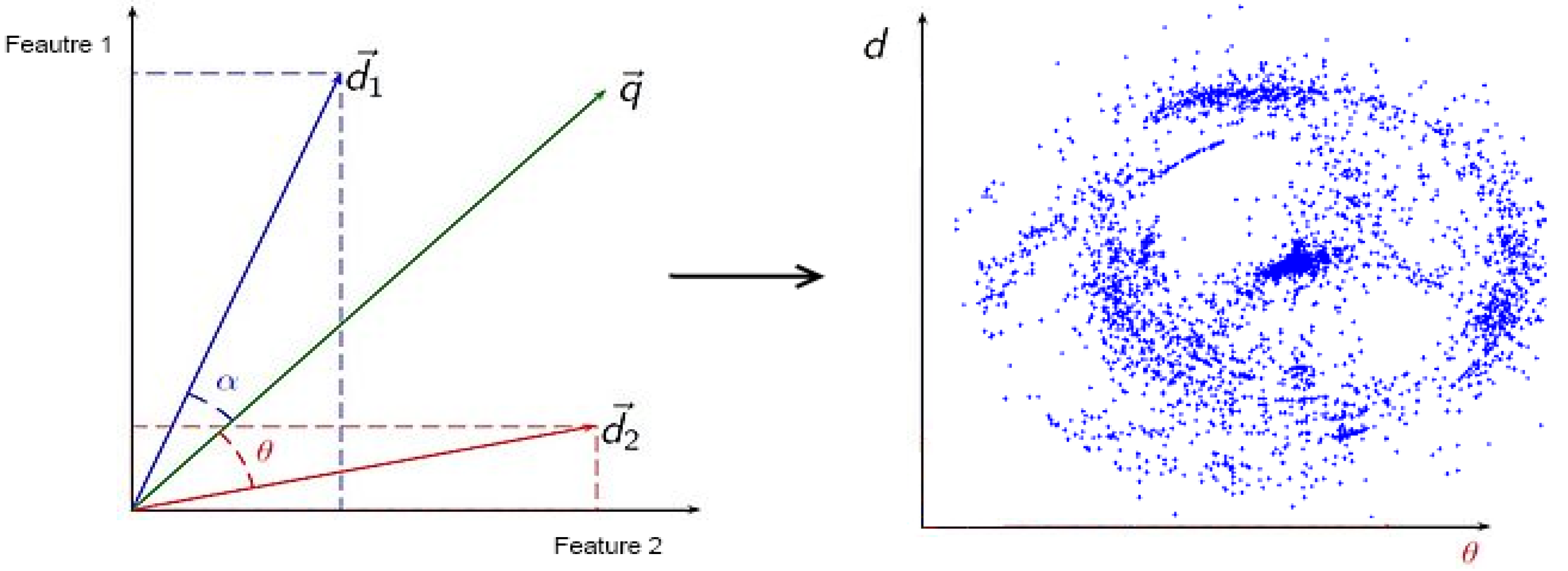
2.6. Similarity Space Transformation

The spectral pattern recognition techniques could characterize the properties of any phenomenon by using inter-band information and defining the spectral similarity measures [33,34]. Deterministic similarity measures were used to project the multispectral data into a new similarity space with minimum knowledge (e.g., the spectral mean vector) about classes of interest [41]. In this new space, the pixels corresponding to any class will obtain similar values [42]. In addition to low computational requirements, they could minimize some undesirable physical effects including noises, illumination, and topographic variation on intra-band spectral data [34,43]. Spectral Angle, Distance, and Correlation values have been used for material mapping by using spectral matching techniques [44]. The spectral similarity functions map the original reflectance or radiance data into a new space for a specific class of interest [33]. In this paper, the multi-spectral data are transformed into the similarity spaces using several measures such as Spectral Distance-Angl-Correlatio-Value (SDACV) (Figure 3) [34].
Figure 3. Spectral angle (θ) and distance similarity measures (d). Vector di and q represent the value of bi-temporal pair of images and reference change vector respectively.
Remotesensing 07 12829 g003
dist = x , μ ch = i = 1 L ( x i μ ch i ) 2
angle = cos 1 ( x . μ ch x μ ch )
Where dist and angle are the spectral distance and angle between any multi-temporal pixel x and the mean vector μch of change classes [33,34].
corr = 1 L 1 ( i = 1 L ( x i μ x ) ( μ ch i μ ¯ ch ) σ x σ μ ch )
spec _ value = ( dist 2 ( 1 corr ) 2
Where corr and spec_value are the correlation and spectral value between any multi-temporal pixel x and the mean vector uch of change classes. In Equations (13) and (15), L is number of multi-temporal image bands.

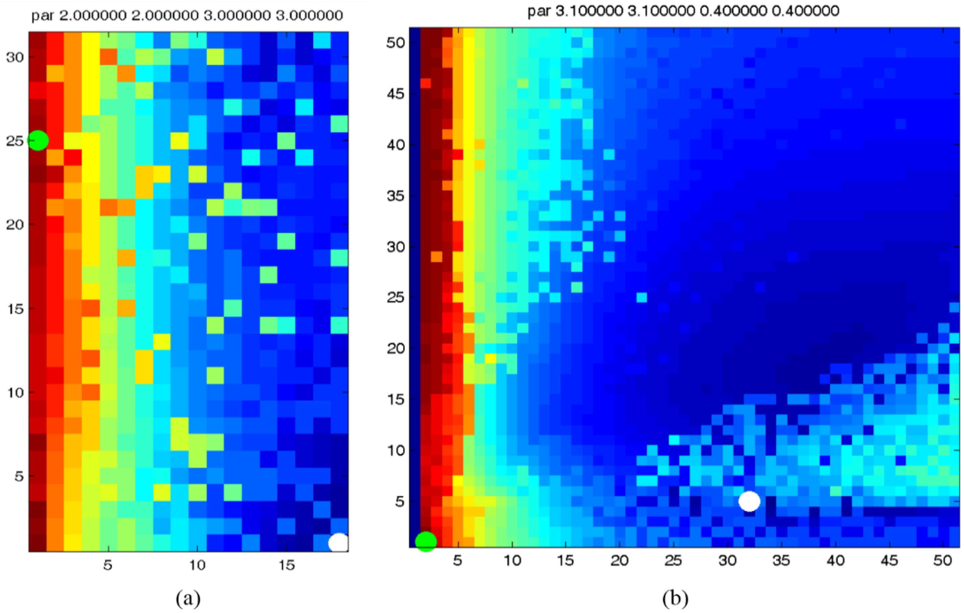
2.7. Improved Kernel Parameter Selection

For almost all kernel-based algorithms, the selection of the parameters plays an essential role in the efficiency of algorithm. In this paper, the kernel K-means clustering the kernel parameters are tuned automatically by optimizing a criterion with the nature of geometrical and similarity in Hilbert space. The geometrical part of this criterion, tries to cluster the multi-temporal image with an optimal geometrical configuration. To achieve this purpose, the difference between the average cluster distance and the centers in the feature space is minimized and used as a geometrical criterion [17,45]. Moreover, the similarity part of the criterion is minimizing the resemblance between the clusters. Both of these geometrical and similarity parts of the criterion are combined linearly with C1 and C2 coefficients. These parameters are determined during the optimization process. These developed criterion lead to an optimal selection of kernel parameters. The set of retained kernel parameters θ°pt is:
θ opt = arg min { C 1 × G + C 2 × S }
G = [ 1 n q = 1 K i ϵ π q d ( φ ( x i ) , μ q ) π q π l d ( μ q , μ l ) ]
S = [ ( 1 1 n 1 ( i ϵ π q j ϵ π l ( φ ( x i ) μ q ) ( φ ( x j ) μ l ) σ q σ l ) ) 2 + i ϵ π q j ϵ π l d ( φ ( x i ) , φ ( x j ) ) 2 2 ]
In Equation (17), G and S are the geometrical and similarity parts of proposed cost function. To estimate this quantity; the kernel K-means is wrapped on the given pseudo-training set by varying C1; C2; θ. The parameters minimizing the Equation (17); are used as optimum kernel parameter in kernel clustering algorithm; by assigning an unknown pixel x’ to the cluster whose centroid satisfies   arg   min x c d ( φ ( x ) , φ ( x C ) ) . This can be seen as a nonlinear minimum distance classification [45]. A great number of kernel functions exist and it is difficult to explain their individual characteristics. As shown in [46] two kinds of kernels may be defined:
(1)
Local kernels. In this kernel type, only the data that are close or in the proximity of each others have an influence on the kernel values. Basically, all kernels that are based on a distance function are local kernels. Examples of typical local kernels are: Radial Basis, KMOD, and Inverse Multi-quadric.
Radial   Basis   Function :   K ( x , x ) = exp ( g x x 2 ) KMOD : K ( x , x ) = exp ( 1 1 + x x 1 ) Inverse   Multiquadratic :   K ( x , x ) = exp ( 1 x x 2 + 1 )
(2)
Global kernels. In this kernel type, samples that are far away from each other still have an influence on the kernel value. All kernels based on the dot-product are global:
Linear :   K ( x , x ) = x . x Polynomial : K ( x , x ) = ( x . x + 1 ) p Sigmodi : K ( x , x ) = tanh ( x . x + 1 )
In this paper we used linear, polynomial, RBF, and sigmoid functions as kernels in proposed kernel-based change detection methods. Different kernels can be used to accommodate the wide-range of nonlinearities that may occur in the various datasets. Therefore, according to the complexity of the remote sensing datasets, an optimal kernel selection process must be carried out. Typically, this selection process could be done by optimizing a certain cost function related to an issue that must be resolved in remote sensing applications. As stated earlier, in this paper we used an improved cost function with the nature of geometrical and similarity in Hilbert space for extracting the optimum kernel types and kernel parameters.

3. Experiments

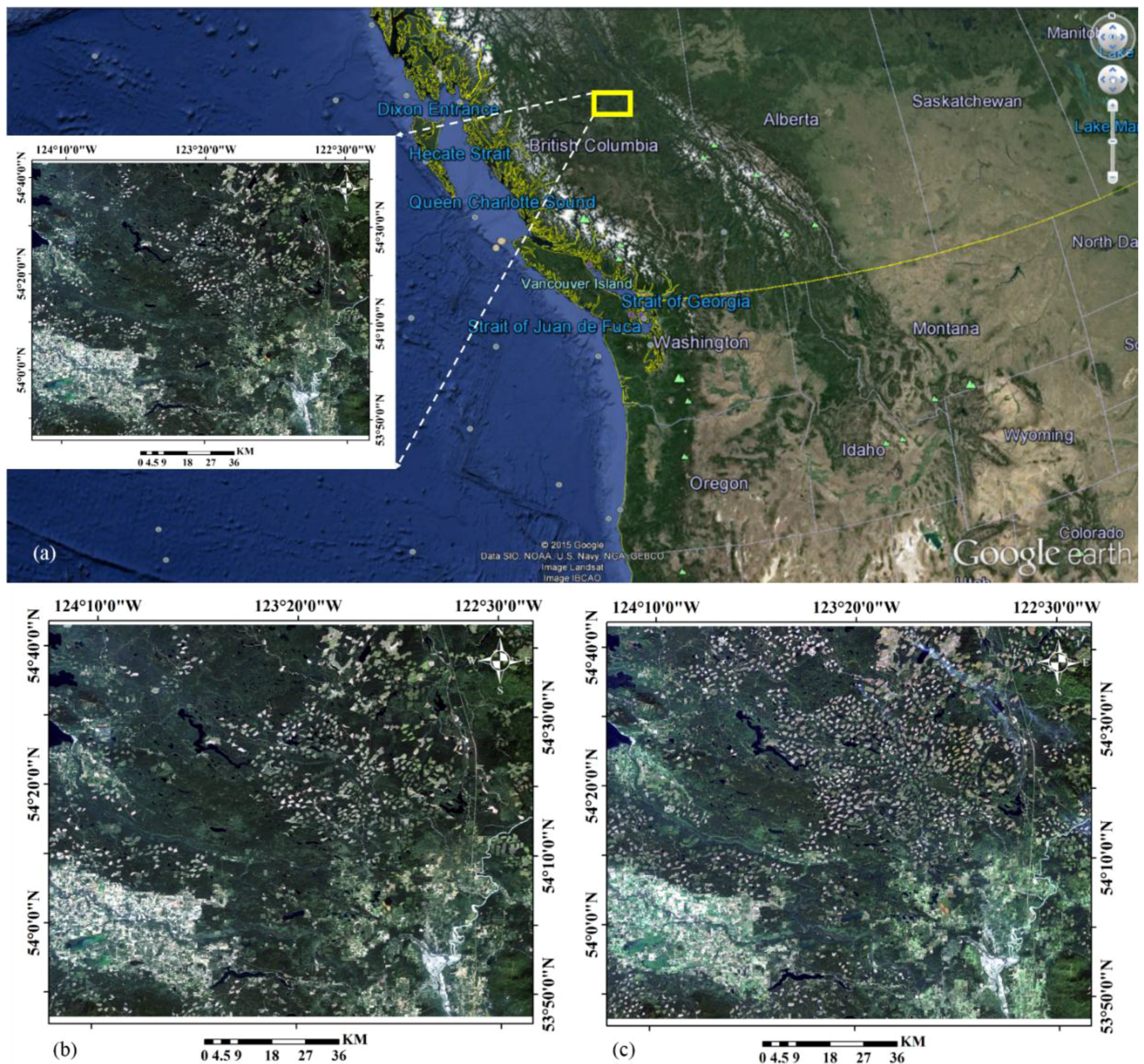
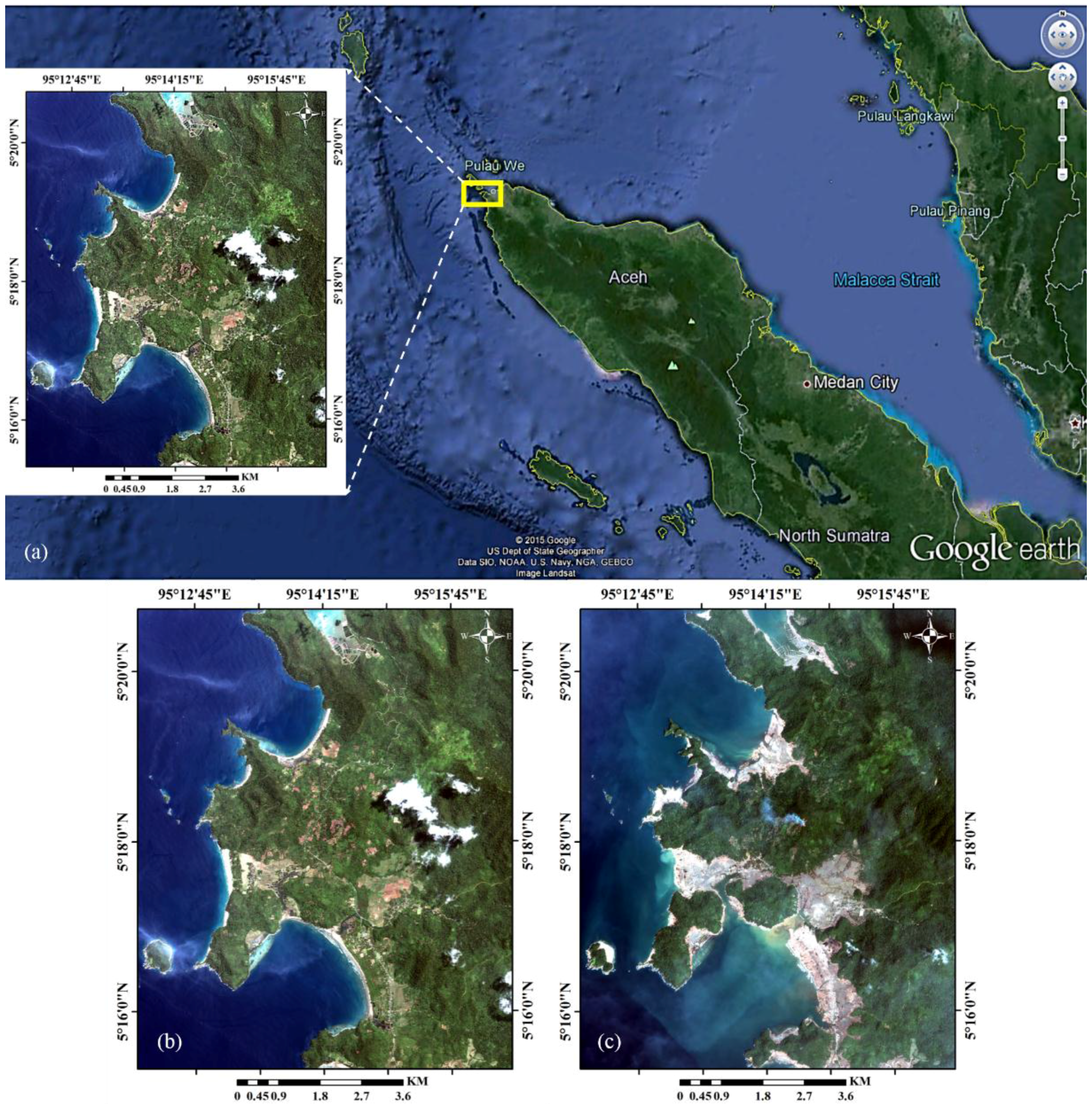
3.1. Remote Sensing Data

In order to assess the effectiveness of the proposed approach, we considered two different data sets made up of multi-temporal-multispectral images acquired by the Landsat TM/ETM+ and Quickbird imageries. The first dataset refers to an area in Prince George area in Northern British Columbia, Canada, whereas the second one concerns a coastal area of Sumatra, Indonesia.
Figure 4. True color images acquired by Landsat satellite over the Prince George area in Northern British Columbia (a), before (b) and after (c) the logging activities on 1990 and 1999, respectively [47].
Remotesensing 07 12829 g004
In the first dataset, the logging activities in 1990 occurred in Prince George area in Northern British Columbia, Canada causing environmental damage in this region. In order to perform our change detection process and extract the deforestation areas, the Landsat imagery are used in two time periods; before and after the logging. The images have been acquired in 1990 and 1999 by Landsat-5 TM and Landsat-7 ETM+, respectively. This multi-date images have 30 m spatial resolution and seven spectral bands. The true color images of before and after the logging activities are shown in Figure 4.
In the second dataset, the 2004 Indian Ocean earthquake was an undersea mega thrust earthquake that occurred at 00:58:53 UTC on Sunday, 26 December 2004, with an epicentre off the west coast of Sumatra, Indonesia [48]. It was one of the deadliest natural disasters recorded in history [14]. To extract the destroyed areas affected by tsunami in coastal area, the Quickbird imagery are used in two time periods; before and after the tsunami. The images have been acquired in December 2004 and January 2005 respectively. This multi-date images have 2.5 m spatial resolution and four spectral bands of red, blue, green, and near-infrared. The true color images of before and after the tsunami are shown in Figure 5.
Figure 5. True color images acquired by Quickbird satellite over Indonesia (a), before and after the tsunami on April 2004 (b) and January 2005 (c) [49].
Remotesensing 07 12829 g005
One of the main reasons for using these two data sets is that, in both of them, due to the occurrence of natural or planned disaster, a change has been created in the natural environment. Also, the purpose of this paper is to provide an efficient and accurate method to monitor the environmental changes using each type of remotely-sensed data.

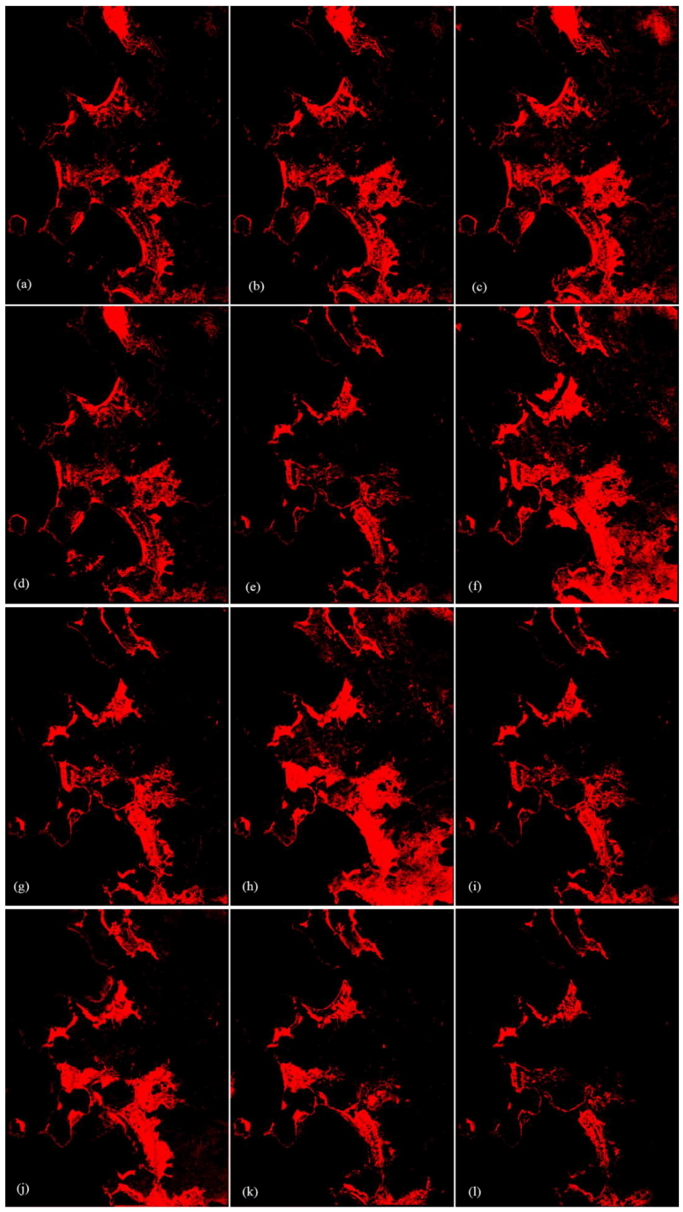
3.2. Experimental Results

To evaluate the efficiency of the proposed method, various assessments are carried out: (1) Accuracy analysis of Heap-SPC approach using the proposed kernel-based algorithm in spectral space; (2) a comparative evaluation of two methods for calculating the difference image such as DFSS-SIM and DFHS-SIM approaches in similarity space; (3) sensitivity analysis of proposed kernel-based method with respect to kernels’ types and their parameters; (4) a comparative analysis between the proposed kernel-based change detection method and SVDD-based change detection method; (5) evaluation of usefulness of the similarity space versus spectral space for implementing the proposed kernel-based change detection algorithm; and (6) computational cost and accuracy analysis of proposed methods against the conventional change detection methods, namely, the MNF (Minimum Noise Fraction) change detection method, the ICA (Independent Component Analysis) based change detection method, SAM (Spectral Angle Mapper), Image Subtraction change detection, and Image Rationing change detection methods.
In proposed kernel-based change detection algorithm and SVDD-based change detection method, the range of kernel parameters is as follows: (1) RBF kernel and sigmoid kernel bandwidth variation ranges are (0.1, 5) with the rate of change 0.1; (2) the degree of polynomial kernel variation range is (0, 5) with the rate of change 1 and (3) single-time and cross-time kernel parameters variation interval used in DFHS approach, are considered (0, 5) with a change rate value of 0.1 at each step. All the change intervals used in the grid search method done by automatic statistical method using L2-norm distance to estimate the optimal parameters for this interval.
To evaluate the proposed algorithm, the test data have been extracted from the images by visually comparing the multi-temporal images. In Quickbird and Landsat data sets, the number of test samples for change class was 4959 and 4727 pixels and for no-change class was 3343 and 4575 pixels, respectively. These samples are selected such that they spread over the entire area that the effects of sun angle and topography should be carefully considered in the analysis. Two criteria based on kappa coefficient of agreement and Overall Accuracy (OA) were used for quantitative accuracy analysis of the results.

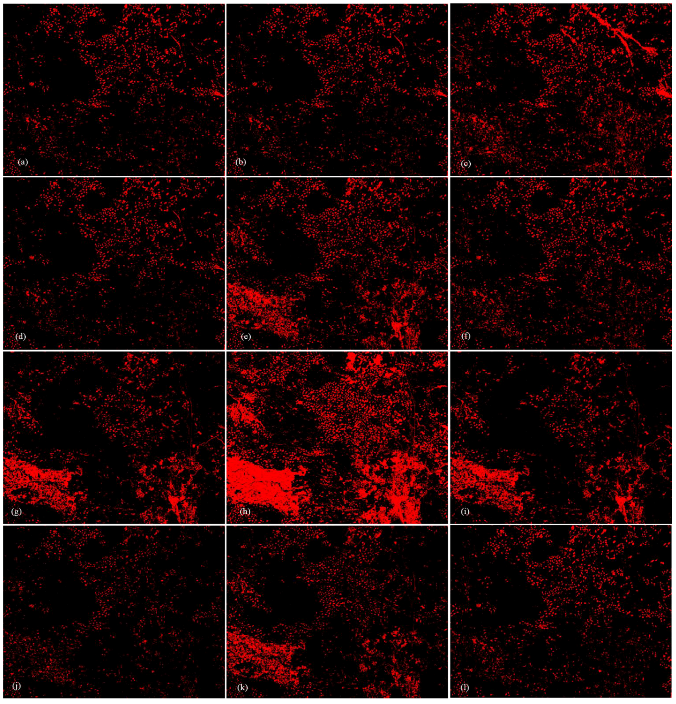
3.2.1. Proposed Kernel-Based CD Method

In this section, the proposed kernel-based CD method with two differencing approaches (DFSS-SIM and DFHS-SIM) are implemented and analyzed on Quickbird and Landsat data sets. In the first step, all pixels of the images are transferred into the similarity space. Then, difference images were calculated via DFSS-SIM and DFHS-SIM approach. In the next step, the difference images are used as input to the kernel K-means clustering algorithm. Then, after the selection of optimum parameters, a clustering algorithm is used to extract the precise training set. These samples are used for training the KMD classifier. The KMD classifier is then employed to separate the change and no-change pixels. The accuracy evaluation of proposed CD method in both data sets using DFSS-SIM and DFHS-SIM differencing approach are presented in Table 1.
Table 1. The accuracy analysis of proposed CD method using DFSS-SIM and DFHS-SIM approaches.
ClassifierInput BandsKernel TypeDFSS-SIMDFHS-SIM
Quickbird LandsatQuickbirdLandsatQuickbirdLandsat
KappaOAKappaOAKappaOAKappaOA
KMD SDACVSDACVLinear0.8590.470.8995.380.8690.620.9096.74
KMD SDACVSDACVPolynomial0.6871.440.7176.490.7073.630.7378.29
KMD SDACVSDACVRBF0.9094.390.8995.670.7478.210.8287.64
KMD SDACVSDACVSigmoid0.8791.810.7985.270.6871.600.8894.58
For Quickbird dataset, the accuracy analysis of DFSS-SIM approach showed that, the best results were obtained by using the DFSS-SIM–RBF scenario (average improvement of ~4% in Kappa coefficient), which is closely followed by the DFSS-SIM-Linear and DFSS-SIM-Sigmoid scenarios. However, the DFSS-SIM-Polynomial scenario did not provide sufficient accuracy. For Landsat dataset, DFSS-SIM-Linear and DFSS-SIM-RBF approaches indicated the same result with a higher accuracy (average improvement of ~14% in Kappa coefficient) than DFSS-SIM-Polynomial and DFSS-SIM-Sigmoid approaches (Table 1). Once again, the RBF kernel yielded higher accuracy than the linear, polynomial and sigmoid kernels. It seems that, when the DFSS-SIM approach is used to calculate the differential image, the separation function between change and no-change classes is similar to a Gaussian function. So in this case, it is convenient to use an RBF kernel.
The accuracy analysis of DFHS-SIM approach showed that, for Quickbird dataset, the best results were obtained by using the DFHS-SIM-Linear approach (average improvement of ~15% in Kappa coefficient) with respect to DFHS-SIM-RBF, DFHS-SIM-Polynomial, and DFHS-SIM-Sigmoid approaches. Also, for Landsat dataset, the best results were obtained by using the DFHS-SIM-Linear approach (average improvement of ~15% in Kappa coefficient) which is closely followed by the DFHS-SIM-Sigmoid and DFHS-SIM-RBF approaches. However, DFHS-SIM–Polynomial scenario did not provide sufficient accuracy. The results showed that, Linear kernel yielded higher accuracy than the RBF, polynomial, and sigmoid kernels. It seems that, when the DFHS-SIM method is used to calculate the differential image, the separation function between change and no-change classes is similar to a linear function. Thus in this case, it is convenient to use a linear kernel.
However, for Quickbird dataset, it can be noted that, the DFHS-SIM scenario (average improvement of ~1.5% in Kappa coefficient) performed slightly better than the DFSS-SIM scenario in the case of linear and polynomial kernels, but in the case of RBF and sigmoid kernel, DFSS-SIM scenario has a higher accuracy (average improvement of ~17.5% in Kappa coefficient) than DFHS-SIM scenario. For Landsat dataset, it can be noted that, the DFHS-SIM scenario (average improvement of ~4% in Kappa coefficient) performed slightly better than the DFSS-SIM scenario in almost all the cases except RBF kernel. Although, OA and Kappa measurements were unbalanced, suggesting that high values of false detections were produced. Consequently, for Quickbird dataset and in the case of using polynomial kernel, it is better that first, multi-temporal images are transferred to the Hilbert space, then these images are subtracted pixel-by-pixel from each other, in order to obtain the difference image. But in the case of using sigmoid kernel, it is better to use the DFSS-SIM approach to obtain the final difference image. But, for Landsat dataset and in the case of using polynomial and sigmoid kernels, it is better that, multi-temporal images are first transferred into the Hilbert space. These images, are then subtracted pixel-by-pixel in order to obtain the difference image. But in the case of using RBF kernel, it is better to use the DFSS-SIM approach for obtaining the final difference image.
In Heap-SPC approach, before and after images are stacked together and transformed into Hilbert space. To increase the accuracy of the final change maps, in addition to the original bands, some features and spectral indexes were extracted from Quickbird and Landsat data sets. In the case of Quickbird dataset, some features based on the co-occurrence matrix of all the bands in each of the multi-temporal images are extracted. Since, both study areas include vegetation cover, the NDVI index is therefore helpful for separation of two classes of interest. Then, a filter-based feature selection method (correlation analysis between bands) is used to select the optimal features. Finally, the best selected features for Quickbird data sets are bands 1, 2, 3, and 4, the mean and variance of band 1 and NDVI. In the case of Landsat dataset, the best selected features are bands 1, 3, 4, 5, 7, and NDVI. The accuracy evaluation of the proposed CD method in both data sets using Heap-SPC approach are presented in Table 2.
Table 2. The accuracy analysis of proposed CD method using Heap-SPC approach.
ClassifierInput BandsKernel TypeHeap-SPC
QuickbirdLandsatQuickbirdLandsat
KappaO.A.Kappa O.A.
KMD Bands 1,2,3,4, µ_b1, σ_b1, NDVIBands 1,3,4,5,7 NDVILinear0.9094.890.7883.63
KMD Bands 1,2,3,4, µ_b1, σ_b1, NDVIBands 1,3,4,5,7 NDVIPolynomial0.8387.320.8086.12
KMD Bands 1,2,3,4, µ_b1, σ_b1, NDVIBands 1,3,4,5,7 NDVIRBF0.9296.730.7783.14
KMD Bands 1,2,3,4, µ_b1, σ_b1, NDVIBands 1,3,4,5,7 NDVISigmoid0.8185.470.7075.40
The accuracy analysis of Heap-SPC approach showed that, for Quickbird dataset, the best results were obtained by using the Heap-SPC–RBF scenario (average improvement of ~7% in Kappa coefficient), which is closely followed by the Heap-SPC-Linear, Heap-SPC-Polynomial and Heap-SPC-Sigmoid approaches. Therefore, RBF kernel yielded higher accuracy than the linear, polynomial, and sigmoid kernels. It seems that, in this case, when the Heap-SPC approach is used to transfer the multi-temporal image to Hilbert space, the separation function between change and no-change classes is similar to a Gaussian function. So in this case, it is convenient to use an RBF kernel. But, For Landsat dataset, the best results were achieved by using the Heap-SPC-Polynomial scenario (average improvement of ~5% in Kappa coefficient), which is closely followed by the Heap-SPC-Linear, Heap-SPC-RBF and Heap-SPC-Sigmoid approaches. So, polynomial kernel yielded higher accuracy than the linear, RBF, and sigmoid kernels. It seems that, in this case, when the Heap-SPC approach used to transfer the multi-temporal image to Hilbert space, the separation function between change and no-change classes is similar to a Gaussian function. So in this case, it is convenient to use a RBF kernel.
By comparing the results showed in Table 1 and Table 2, it can be noted that, for Quickbird datasets, Heap-SPC approach (average improvement of ~7% in Kappa coefficient) performed slightly better than the DFSS-SIM scenario in almost all the cases except the sigmoid kernel. But, Heap-SPC approach (average improvement of ~12% in Kappa coefficient) performed better than the DFHS-SIM scenario in the case of all kernel types. For Landsat dataset, DFSS-SIM and DFHS-SIM approaches (average improvement of ~11% and 12% in Kappa coefficient) performed better than the Heap-SPC scenario in almost all the cases except the polynomial kernel, respectively. It can be concluded that, for Landsat datasets, implementation of proposed CD method in similarity space has provided better results than spectral space.

3.2.2. Proposed SVDD-Based CD Method

In this method, each of the multi-temporal images are transferred to the Hilbert space by using kernel functions. Then these transferred multi-temporal images stacked together in a higher dimensional space and used as input to the SVDD-based CD algorithm. By using the pseudo training samples obtained from clustering algorithm, the SVDD-based CD method was trained. In the next step, grid-searching and cross validation method was used for selecting the best SVDD parameters. Finally, SVDD-based discrimination function is used to separate the change and no-change pixels. The accuracy evaluation of the proposed SVDD-based CD method is presented in Table 3.
Table 3. The accuracy analysis of proposed SVDD-based CD method.
CD MethodInput BandsKernel TypeQuickbirdLandsat
QuickbirdLandsatKappa O.A.Kappa O.A.
SVDD-basedBands 1,2,3,4, µ_b1, σ_b1, NDVIBands 1,3,4,5,7 NDVILinear0.8690.280.8490.54
SVDD-basedBands 1,2,3,4, µ_b1, σ_b1, NDVIBands 1,3,4,5,7 NDVIPolynomial0.8892.070.8288.41
SVDD-basedBands 1,2,3,4, µ_b1, σ_b1, NDVIBands 1,3,4,5,7 NDVIRBF0.9195.280.9096.22
SVDD-basedBands 1,2,3,4, µ_b1, σ_b1, NDVIBands 1,3,4,5,7 NDVISigmoid0.8084.110.7479.35
The accuracy assessment of SVDD-based CD method showed that, for Quickbird and Landsat datasets, using the RBF kernel function gives a higher accuracy than using other kernel types. Once again, the RBF kernel function perform better than other kernel types. It seems that, in proposed SVDD-based CD method, the separation function between change and no-change classes is similar to a Gaussian function. So, it can be concluded that, for both datasets, the RBF kernel is the best choice for the proposed SVDD-based CD method and has a higher accuracy than other kernel types (Table 3).
By comparing the results showed in Table 1, Table 2 and Table 3, it can be noted that: for Quickbird dataset, Heap-SPC approach (average improvement of ~2% in Kappa coefficient) performed slightly better than the SVDD-based CD method in almost all the cases except the polynomial kernel. The SVDD-based CD method (average improvement of ~7% in Kappa coefficient) performed better than the DFSS-SIM approach in almost all the cases except the sigmoid kernel. SVDD-based CD and DFHS-SIM approaches indicated the same result in the case of RBF kernel. But, SVDD-based CD method (average improvement of ~16% in Kappa coefficient) performed better than the DFHS-SIM approach in other kernel types.
For Landsat dataset, SVDD-based CD method (average improvement of ~6% in Kappa coefficient) performed better than the Heap-SPC approach for all kernel types. In the case of linear and sigmoid kernels, DFSS-SIM and DFHS-SIM approaches (average improvement of ~5% and 10% in Kappa coefficient) performed better than the SVDD-based CD method, respectively. The SVDD-based CD and DFSS-SIM approaches indicated the same result in the case of RBF kernel. But, SVDD-based CD method (improvement of ~11% and 9% in Kappa coefficient) performed better than the DFSS-SIM and DFHS-SIM approaches for polynomial kernel. Finally, in the case of RBF kernel, SVDD-based CD method (improvement of ~8% in Kappa coefficient) performed better than the DFHS-SIM approach.
Several discussions can be deduced from the accuracy assessment of proposed CD methods on both datasets. In most cases, the proposed kernel-based CD framework has better results when compared with SVDD-based CD method. We can, consequently, conclude that in the proposed hybrid CD method based on CVA, KKMC, and KMD approaches, each part of the algorithms initialized the other part. So, this algorithm converges quickly and more accurate results are obtained. The initial values, calculated at each stage of the algorithm, increased the convergence and accuracy of the results. In the proposed kernel-based algorithm, the training procedure of KMD classifier performed by precise training samples. While the SVDD-based CD method could not extract accurate training samples from initial samples and trained directly with pseudo-training samples.
In Figure 6, for Quickbird dataset, the change maps obtained from DFSS-SIM-Linear (a), DFSS-SIM-RBF (b), DFSS-SIM-Sigmoid (c), DFHS-SIM-Linear (d), Heap-SPC-Linear (e), Heap-SPC-Polynomial (f), Heap-SPC-RBF (g), Heap-SPC-Sigmoid (h), SVDD-Linear (i), SVDD-Polynomial (j), SVDD-RBF (k), SVDD-Sigmoid (l) approaches are shown, respectively. The black color indicates the no-change class while the red color indicates the no-change class.
As it can be seen in Figure 6f and Figure 6h, in change maps obtained from Heap-SPC-Polynomial and Heap-SPC-Sigmoid approaches, the ocean and the forest areas are somewhat detected as the change. There is clear changes for ocean and forest which are related to the normal raging in ocean and atmospheric conditions respectively; but they are not considered as change classes. The change map shown in Figure 6a–d,i, obtained from DFSS-SIM–Linear, DFSS-SIM–RBF, DFSS-SIM-Sigmoid, DFHS-SIM-Linear approaches, the ocean areas located in the north of the study area are also detected as the change. These changes are only due to the raging of ocean at the tsunami struck but they are not considered as change classes. However, the change map shown in Figure 6e,g,j,k, in change map obtained from Heap-SPC-Linear, Heap-SPC-RBF, SVDD-Polynomial, and SVDD-RBF approaches got limited isolated pixels and they were less noisy in essence and better results have been achieved.
In Figure 7, for Landsat dataset, the change maps obtained from DFSS-SIM-Linear (a), DFSS-SIM–RBF (b), DFSS-SIM-Sigmoid (c), DFHS-SIM-Linear (d), DFHS-SIM–RBF (e), DFHS-SIM-Sigmoid (f), Heap-SPC-Linear (g), Heap-SPC-Polynomial (h), Heap-SPC-RBF (i), SVDD-Linear (j), SVDD-Polynomial (k), SVDD-RBF (l) approaches are shown, respectively.
Figure 6. Change maps obtained from (a) DFSS-SIM-Linear, (b) DFSS-SIM-RBF, (c) DFSS-SIM-Sigmoid, (d) DFHS-SIM-Linear, (e) Heap-SPC-Linear, (f) Heap-SPC-Polynomial, (g) Heap-SPC-RBF, (h) Heap-SPC-Sigmoid, (i) SVDD-Linear, (j) SVDD-Polynomial, (k) SVDD-RBF, (l) SVDD-Sigmoid approaches.
Remotesensing 07 12829 g006
Figure 7. Change maps obtained from (a) DFSS-SIM-Linear, (b) DFSS-SIM-RBF, (c) DFSS-SIM-Sigmoid, (d) DFHS-SIM-Linear, (e) DFHS-SIM-RBF, (f) DFHS-SIM-Sigmoid, (g) Heap-SPC-Linear, (h) Heap-SPC-Polynomial, (i) Heap-SPC-RBF, (j) SVDD-Linear, (k) SVDD-Polynomial, (l) SVDD-RBF approaches.
Remotesensing 07 12829 g007
As it can be seen in Figure 7e,g–i,k, change maps obtained from DFHS-SIM–RBF, Heap-SPC-Linear, Heap-SPC-Polynomial, Heap-SPC-RBF, and SVDD-Polynomial methods, the agricultural areas in the southwest of study area are somewhat noisy. These changes are only due to the seasonal change and variety of cultures but they are not considered as change classes. The change map shown in Figure 7c, obtained from DFSS-SIM-Sigmoid approach, the forest areas in the background of the study area are somewhat noisy. These changes are only due to the atmospheric condition. However, the change map shown in Figure 7a,b,d,f,j,l obtained from DFSS-SIM-Linear, DFSS-SIM-RBF, DFHS-SIM-Linear, DFHS-SIM-Sigmoid, SVDD-Linear, and SVDD-RBF methods got limited isolated pixels and they were less noisy in essence and better results have been achieved.
In order to compare our results with the respective outputs from other similar researches, the experimental results of kernel-based CD methods were evaluated. Gustavo Camps-Valls et al. [28,35] proposed two kernel-based CD methods including (1) kernel-based image differencing and image ratioing CD methods and (2) SVMs based and SVDD based multi-temporal image classifiers. Synthetic and real remote sensing data sets were used for analyzing the performance of the proposed methodological framework based on kernels.
It is worth mentioning that implementation of algorithm and flowchart of this framework are quite different with our proposed approach. Several conclusions can be derived from accuracy assessment on synthetic dataset. In all cases, the RBF kernel outperformed the linear kernel. In multi-temporal image classification, the best kernel classifier is constituted by the cross-terms kernel because it includes the temporal information of image evolution. In change detection problems, the best results were obtained by using the difference kernel. SVMs generally works slightly better than the SVDD. In all cases and scenes, it becomes obvious that the use of the RBF kernel provides much better results than the linear kernel. SVMs classifier shows the best results; however, SVDD classifier can also produce stable and robust outcomes, which confirms their suitability to application scenarios in which incomplete or partially complete information is available [28,35]. By comparing our results illustrated in Section 3.2.1 and Section 3.2.2, it can be concluded that the outcome of these works are in agreement with our main findings.
In optimum kernel type and kernel parameter selection of kernel clustering algorithm, these parameters are tuned automatically by optimizing an improved cost function with the nature of geometrical and spectral similarity in kernel space. This optimization process runs for all kernel types so that the optimized kernel parameter and the corresponding kernel type that minimize the cost function to be determined. The procedure of optimal single-time and cross-time RBF kernel parameters selection corresponding to maximum value and minimum value of cost function in the DFHS-SIM-RBF approach is shown in Figure 8. For this purpose, single-time and cross-time parameters of composite kernel defined in Equation (17), were calculated using grid searching method in such a way for the value of the cost function to be minimized [33,36]. This result illustrates the joint optimization of σsinger and σcross (DFHS-SIM-RBF). The proposed cost function showed detectable and appropriate global minima.
As seen in Figure 8; the white marks are placed to minimize the proposed cost function and green marks are the location of the maximum value of the proposed cost function for Quickbird and Landsat data sets. Therefore; the parameters θ = { σ single , σ cross } that the cost function to be minimized for them can be selected. By analyzing the results it can be concluded that for both data sets; for low bandwidth values; the change and no-change clusters are not separable and the spectral similarity of clusters is overestimated. For wider bandwidths; the similarity value between change and no-change clusters is underestimated. The optimal separability between clusters is reached when the cross kernel parameters is in the range of the average Euclidean distance and average similarity value among pixels within clusters.
Figure 8. Optimal multi-temporal cross kernel parameters selection in DFHS-RBF approach for Quickbird (a) and Landsat (b) data sets.
Remotesensing 07 12829 g008

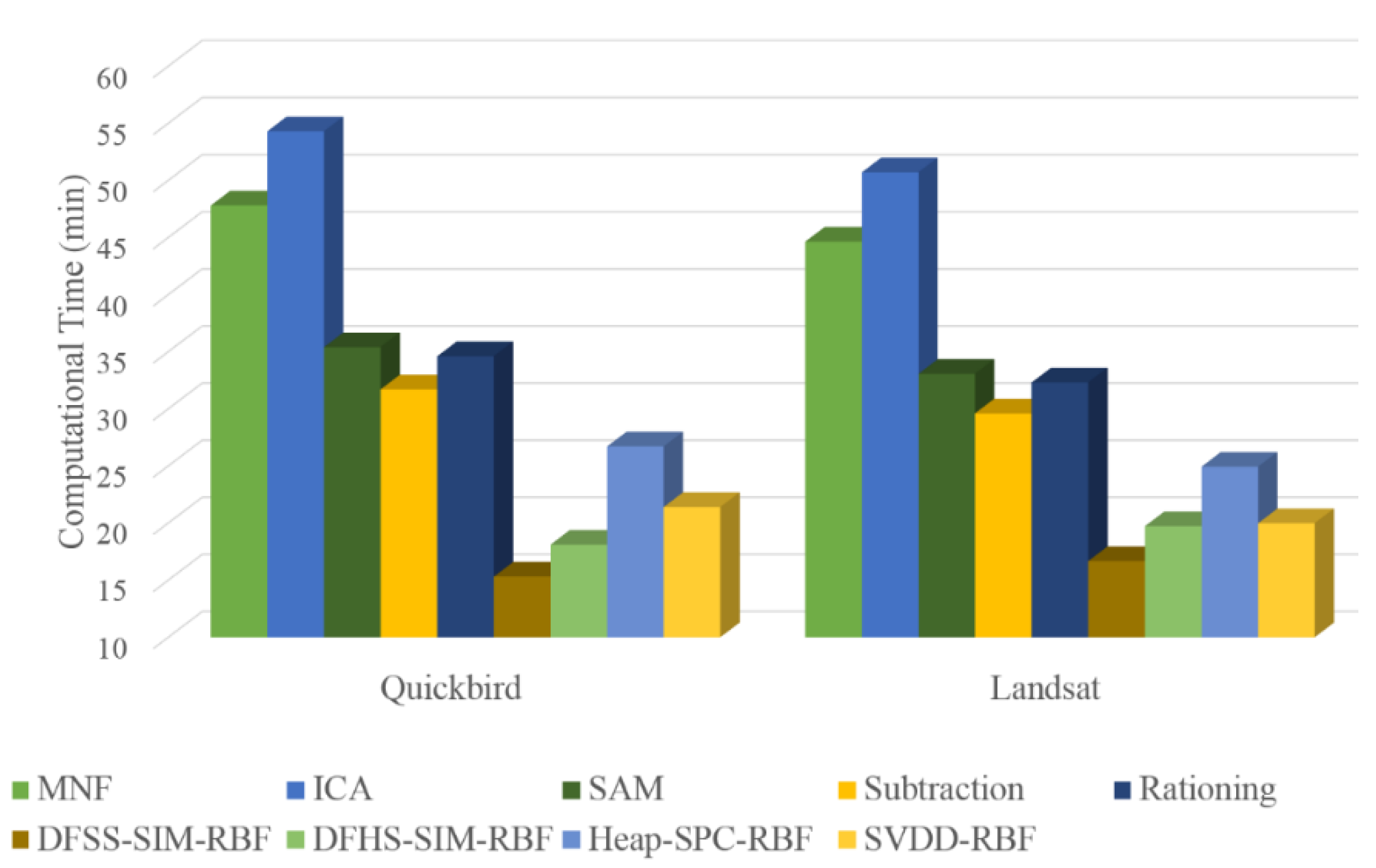
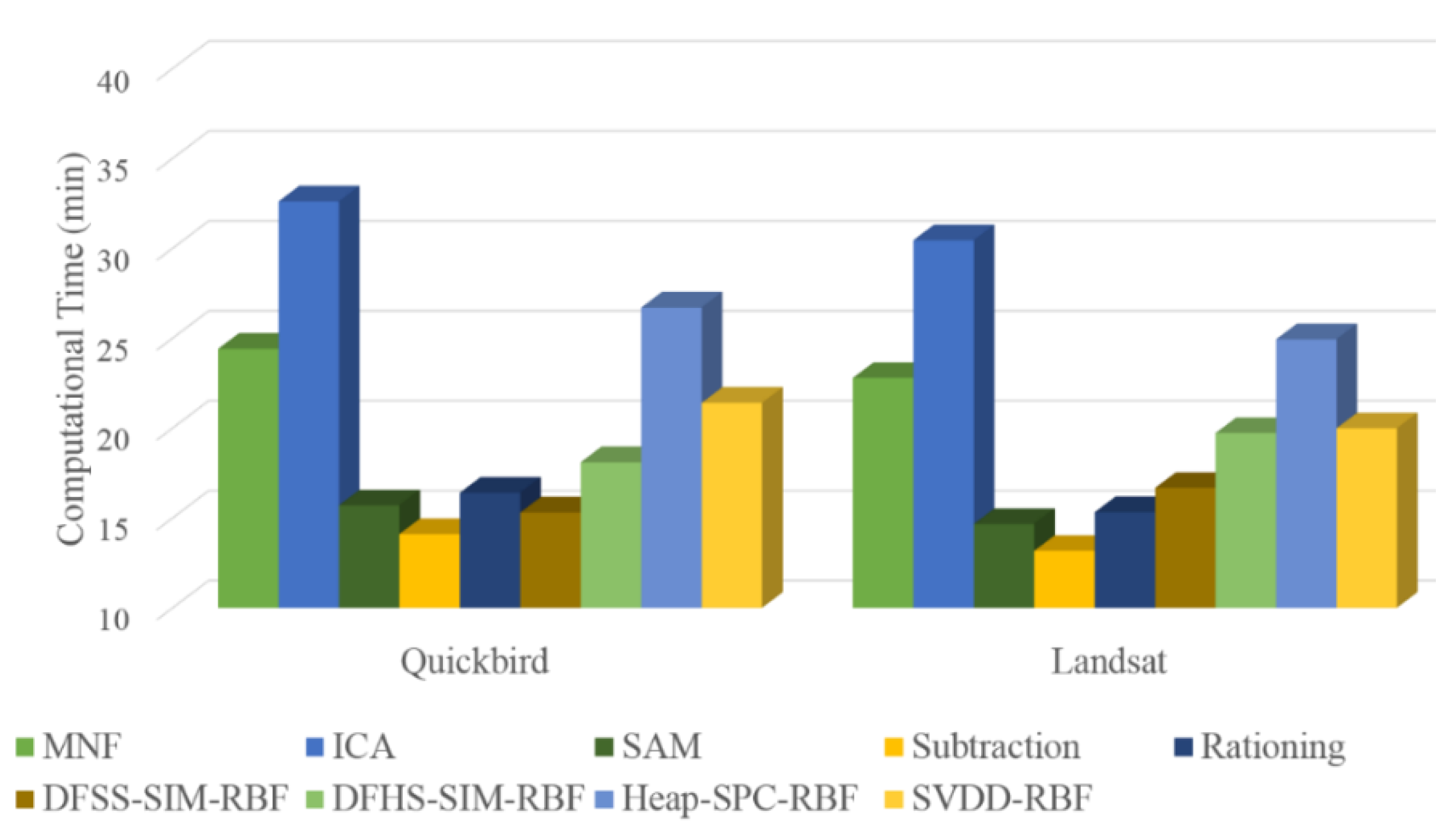
3.2.3. Conventional CD Method

In order to assess the performance of the proposed hybrid CD algorithms, we compared this technique with well-known change detection methods, namely, the MNF (Minimum Noise Fraction) CD method [50], the ICA (Independent Component Analysis) based CD method [51], SAM (Spectral Angle Mapper) [52], Image Subtraction CD [9,53] and Image Rationing CD methods [53,54]. These methods are implemented and tested on the same data in spectral space.
Table 4. The Comparative analysis of conventional CD and proposed CD methods.
CD MethodInput BandsQuickbird Landsat
QuickbirdLandsat
KappaO.A.KappaO.A.
MNF TransformBands 1,2,3,4, µ_b1, σ_b1, NDVIBands 1,3,4,5,7 NDVI0.8491.600.6472.97
ICA TransformBands 1,2,3,4, µ_b1, σ_b1, NDVIBands 1,3,4,5,7 NDVI0.6885.480.6675.54
Spectral Angle MapperBands 1,2,3,4, µ_b1, σ_b1, NDVIBands 1,3,4,5,7 NDVI0.6075.380.7787.80
Image SubtractionBands 1,2,3,4, µ_b1, σ_b1, NDVIBands 1,3,4,5,7 NDVI0.6986.570.6169.40
Image RationingBands 1,2,3,4, µ_b1, σ_b1, NDVIBands 1,3,4,5,7 NDVI0.6176.450.6372.17
DFSS-SIM-RBFSDACVSDACV0.9094.390.8995.67
DFHS-SIM-RBFSDACVSDACV0.7478.210.8287.64
Heap-SPC-RBFBands 1,2,3,4, µ_b1, σ_b1, NDVIBands 1,3,4,5,7 NDVI0.9296.730.7783.14
SVDD-RBFBands 1,2,3,4, µ_b1, σ_b1, NDVIBands 1,3,4,5,7 NDVI0.9195.280.9096.22
These results are presented in Table 4 which show that for both Landsat and Quickbird data sets, all proposed kernel-based methods such as DFSS-SIM-RBF, DFHS-SIM-RBF, Heap-SPC-RBF approaches and SVDD-based CD method have higher accuracy than all well-known CD methods. The classical change detection methods show intermediate level accuracies caused by both the false alarm rate and the weak detection rate when compared to the proposed kernel-based algorithm. Since, spectral difference values for change and no-change classes in the differential image obtained in the spectral space are close to each other, the boundary separation between change and no-change classes is not readily detected. Through transferring this difference image into the Hilbert space with a higher dimension, the separation of these two classes is increased and better results will be achieved. This classical method is extremely sensitive to the noise of data and error of multi-temporal data misregistration. The accuracy of the produced change map is greatly dependent on the selection of appropriate threshold.
Two scenarios were considered in order to compare the computational cost of the proposed kernel-based CD methods, against the computational cost of classical algorithms. The computational runtime of each method presented in Table 4 was estimated. In the first scenario, the computational cost of classical CD methods were calculated with regard to the fact that the thresholding stage made through an operator. Therefore, the required time for selecting the appropriate threshold will be considered in processing time. But in the second scenario, it is assumed that the thresholding stage has already been done for classical CD methods. As a result, the computational cost analyses are only related to the computational runtime of processing cores of proposed and classical methods. However, in both scenarios, the required time for automatic threshold selection is considered in the processing runtime of proposed CD methods. For a fair comparison, all classical and proposed CD methods were implemented in the same programming environment. Since the runtime of the proposed kernel-based methods depend on the time of grid searching process for determining the optimized kernel parameter, therefore, it is assumed that the optimum kernel parameter is already known in both scenarios. The computational cost analysis of classical CD and proposed CD methods for both datasets when threshold is estimated by an operator (first scenario) was given in Figure 9.
Figure 9. Computational cost analysis of classical CD and proposed CD methods for Quickbird and Landsat datasets when thresholding stage made through an operator in classical CD methods (first scenario).
Remotesensing 07 12829 g009
As seen in Figure 9, the computational runtime of proposed methods are less than the classical CD methods. In addition, DFSS-SIM and DFHS-SIM approach have the lowest computational cost compared to other methods. It is evident that the implementation of proposed CD method in similarity space decreases the processing times. Furthermore, the conventional CD methods are largely dependent on the user interaction and are non-automatic. Determination of the exact threshold is very time consuming and requires a skilled operator. The computational cost analysis of classical CD and proposed CD methods for both datasets with the thresholding stage pre-made in classical CD methods (second scenario) are presented in Figure 10.
Figure 10. Computational cost analysis of classical CD and proposed CD methods for Quickbird and Landsat datasets when the thresholding stage was pre-made in classical CD methods (second scenario).
Remotesensing 07 12829 g010
Comparative computational cost analysis of proposed CD method against classical CD methods showed that (See Figure 10), for both datasets, the lowest computational cost was obtained by using the Subtraction method. This is closely followed by the SAM, Ratioing, DFSS-SIM and DFHS-SIM approaches. Although the threshold of the proposed method is selected automatically, the processing time does not significantly change compared to the conventional CD methods. For example, the processing time of DFSS-SIM, DFHS-SIM, Heap-SPC, and SVDD methods is far less than ICA and MNF CD methods. It can be concluded that the implementation of proposed CD method in similarity space decreases the processing times. Consequently, in the absence of a skilled user, the processing time of conventional CD methods greatly increases.

4. Conclusions

In this paper, a kernel-based and hybrid framework is presented for change detection from remotely sensed data in a similarity space. This proposed method shows great flexibility for the problem of change detection by finding nonlinear solutions to the problem. The main issues of the framework have been discussed and resolved. Firstly, the initialization was addressed by finding a threshold on change vector magnitude distribution. A geometrically and spectral similarity inspired cost function has been proposed to estimate the optimal single-time and cross-time kernel parameters. This cost function produces clusters that minimize the similarity and maximize the distance between them. By exploiting a proper initialization, the kernel K-means clustering is used to extract the precise training samples for the two classes of interest. Secondly, by reformulating the simple difference CD method in the Hilbert space, the similarity of the difference image in feature spaces are strongly improved. This is accomplished by three approaches, i.e., DFSS-SIM, DFHS-SIM, and Heap-SPC approaches. Thirdly, multi-temporal images are transformed into the similarity space for increasing the separation between change and no-change classes and decreasing the time of the CD process. Lastly, a new method to estimate the initial value of the RBF kernel parameter in the CD problem was proposed. This method is based on a statistical method using the L2-norm distance and leads to a faster convergence of a grid-searching techniques for selecting the global optimum RBF’s kernel parameter.
Experimental comparisons showed that when only relying on the change’s magnitude, the correct discrimination of the changes becomes a difficult task. This is related to the ambiguity of the measure, as well as to the change’s magnitude one-dimensional representation, which hides the useful information in multi-temporal data. Almost all the classical methods are based on the change vector magnitude analysis and the determination of a threshold for separating the change pixels from the no-change ones. Accordingly, the information between change and no-change pixels in multi-temporal images leads to a one-dimensional change vector. While the proposed method uses all the multi-temporal bands and the mutual information between them. Thus, more information can be extracted to separate the unchanged pixels from changed ones. In contrast, by detecting the changes in higher dimensional feature spaces, the multi-temporal information unfolds into clusters that are easily separable. Such an approach also reduces the preprocessing corrections, for the single time information is considered separately and regularized by the cross-similarity of the scenes.
The proposed approach shows accuracy improvements with respect to classical change detection techniques. This indicates that a better illustration can be obtained by considering cross information between multi-temporal images. This leads to a strong decrease in the false alarm rate, and a slight improvement in the detection rates in produced change maps. As a result, this approach is the most accurate one. Finally, the computational cost analysis showed that implementation of proposed CD method in similarity space decrease the processing times. Further research can be done in the field of combining the multi-sensor data such as optic and radar imageries. Such information can be incorporated in the proposed CD framework by developing specific kernel functions. Types of changes and their change directions can also be considered to extend the use of the proposed CD framework for multi-class change detection.

Acknowledgements

The authors sincerely appreciate the assistance and cooperation of ENVI EXCELIS and PCI Geomatics Companies for making available the multi-temporal Quickbird images of earthquake tsunami in coastal areas of Indonesia and Landsat images of logging activities in Prince George area in Northern British Columbia, Canada, respectively.

Author Contributions

Reza Shah-Hosseini performed the experiments and analyzed the data and wrote the paper with significant contributions from Saeid Homayouni and Abdolreza Safari for conceived and designed the experiments, writing the first draft, interpretation of the results and editing the final manuscript.

Conflicts of Interest

The authors declare no conflict of interest.

References

  1. Singh, A. Review article digital change detection techniques using remotely-sensed data. Int. J. Remote Sens. 1989, 10, 989–1003. [Google Scholar] [CrossRef]
  2. Volpi, M.; Tuia, D.; Camps-Valls, G.; Kanevski, M. Unsupervised change detection with kernels. IEEE Geosci. Remote Sens. Lett. 2012, 9, 1026–1030. [Google Scholar] [CrossRef]
  3. Yamazaki, F.; Matsuoka, M. Remote sensing technologies in post-disaster damage assessment. J. Earthq. Tsunami 2007, 1, 193–210. [Google Scholar] [CrossRef]
  4. Curatola Fernández, G.F.; Obermeier, W.A.; Gerique, A.; López Sandoval, M.F.; Lehnert, L.W.; Thies, B.; Bendix, J. Land cover change in the Andes of Southern Ecuador—Patterns and drivers. Remote Sens. 2015, 7, 2509–2542. [Google Scholar] [CrossRef]
  5. Tewkesbury, A.P.; Comber, A.J.; Tate, N.J.; Lamb, A.; Fisher, P.F. A critical synthesis of remotely sensed optical image change detection techniques. Remote Sens. Environ. 2015, 160, 1–14. [Google Scholar] [CrossRef]
  6. Olthof, I.; Fraser, R.H. Detecting landscape changes in high latitude environments using Landsat trend analysis: 2 Classification. Remote Sens. 2014, 6, 11558–11578. [Google Scholar] [CrossRef]
  7. Karnieli, A.; Qin, Z.; Wu, B.; Panov, N.; Yan, F. Spatio-temporal dynamics of land-use and land-cover in the Mu Us Sandy Land, China, using the change vector analysis technique. Remote Sens. 2014, 6, 9316–9339. [Google Scholar] [CrossRef]
  8. Dai, X.; Khorram, S. The effects of image misregistration on the accuracy of remotely sensed change detection. IEEE Trans. Geos. Remote Sens. 1998, 36, 1566–1577. [Google Scholar]
  9. Mas, J.-F. Monitoring land-cover changes: A comparison of change detection techniques. Int. J. Remote Sens. 1999, 20, 139–152. [Google Scholar] [CrossRef]
  10. Vittek, M.; Brink, A.; Donnay, F.; Simonetti, D.; Desclée, B. Land cover change monitoring using Landsat MSS/TM satellite image data over West Africa between 1975 and 1990. Remote Sens. 2014, 6, 658–676. [Google Scholar] [CrossRef] [Green Version]
  11. Lambin, E.F.; Strahlers, A.H. Change-vector analysis in multi-temporal space: A tool to detect and categorize land-cover change processes using high temporal-resolution satellite data. Remote Sens. Environ. 1994, 48, 231–244. [Google Scholar] [CrossRef]
  12. Camps-Valls, G.; Bruzzone, L. Kernel Methods for Remote Sensing Data Analysis; John Wiley and Sons: West Sussex, UK, 2009. [Google Scholar]
  13. Nemmour, H.; Chibani, Y. Multiple support vector machines for land cover change detection: An application for mapping urban extensions. ISPRS J. Photogramm. Remote Sens. 2006, 61, 125–133. [Google Scholar] [CrossRef]
  14. Li, X.; Yeh, A. Principal component analysis of stacked multi-temporal images for the monitoring of rapid urban expansion in the Pearl River Delta. Int. J. Remote Sens. 1998, 19, 1501–1518. [Google Scholar] [CrossRef]
  15. Pang, S.; Hu, X.; Wang, Z.; Lu, Y. Object-based analysis of airborne LiDAR data for building change detection. Remote Sens. 2014, 6, 10733–10749. [Google Scholar] [CrossRef]
  16. Zhou, J.; Yu, B.; Qin, J. Multi-level spatial analysis for change detection of urban vegetation at individual tree scale. Remote Sens. 2014, 6, 9086–9103. [Google Scholar] [CrossRef]
  17. Volpi, M.; Tuia, D.; Camps-Valls, G.; Kanevski, M. Unsupervised change detection by kernel clustering. Proc. SPIE 2010. [Google Scholar] [CrossRef]
  18. Bovolo, F.; Bruzzone, L.; Marconcini, M. An unsupervised change detection technique based on Bayesian initialization and semisupervised SVM. In Proceedings of the IEEE International Geoscience and Remote Sensing Symposium, Barcelona, Spain, 23–28 July 2007; pp. 2370–2373.
  19. Chen, C.-F.; Son, N.-T.; Chang, N.-B.; Chen, C.-R.; Chang, L.-Y.; Valdez, M.; Centeno, G.; Thompson, C.A.; Aceituno, J.L. Multi-decadal mangrove forest change detection and prediction in Honduras, Central America, with Landsat imagery and a Markov chain model. Remote Sens. 2013, 5, 6408–6426. [Google Scholar] [CrossRef]
  20. Chen, J.; Gong, P.; He, C.; Pu, R.; Shi, P. Land-use/land-cover change detection using improved change-vector analysis. Photogramm. Eng. Remote Sens. 2003, 69, 369–380. [Google Scholar] [CrossRef]
  21. Bruzzone, L.; Prieto, D.F. Automatic analysis of the difference image for unsupervised change detection. IEEE Trans. Geos. Remote Sens. 2000, 38, 1171–1182. [Google Scholar] [CrossRef]
  22. Molina, I.; Martinez, E.; Arquero, A.; Pajares, G.; Sanchez, J. Evaluation of a change detection methodology by MEANS of binary thresholding algorithms and informational fusion processes. Sensors 2012, 12, 3528–3561. [Google Scholar] [CrossRef] [PubMed] [Green Version]
  23. Inglada, J.; Mercier, G. A new statistical similarity measure for change detection in multi-temporal SAR images and its extension to multiscale change analysis. IEEE Trans. Geosci. Remote Sens. 2007, 45, 1432–1445. [Google Scholar] [CrossRef]
  24. Mercier, G.; Derrode, S.; Pieczynski, W.; Nicolas, J.-M.; Joannic-Chardin, A.; Inglada, J. Copula-based stochastic kernels for abrupt change detection. In Proceedings of the IEEE International Geoscience and Remote Sensing Symposium, Denver, CO, USA, 31 July 2006–4 August 2006; pp. 204–207.
  25. Pajares, G. A Hopfield neural network for image change detection. IEEE Trans. Neural Netw. 2006, 17, 1250–1264. [Google Scholar] [CrossRef] [PubMed]
  26. Aach, T.; Kaup, A. Bayesian algorithms for adaptive change detection in image sequences using Markov random fields. Signal Process. Image Commun. 1995, 7, 147–160. [Google Scholar] [CrossRef]
  27. Guorui, M.; Haigang, S.; Pingxiang, L.; Qianqing, Q. A kernel change detection algorithm in remote sense imagery. In Proceedings of the IEEE International Geoscience and Remote Sensing Symposium, Denver, CO, USA, 31 July 2006–4 August 2006; pp. 220–224.
  28. Camps-Valls, G.; Gomez-Chova, L.; Munoz-Mari, J.; Rojo-Alvarez, J.L.; Martinez-Ramon, M. Kernel-based framework for multi-temporal and multisource remote sensing data classification and change detection. IEEE Trans. Geosci. Remote Sens. 2008, 46, 1822–1835. [Google Scholar] [CrossRef]
  29. Longbotham, N.; Pacifici, F.; Glenn, T.; Zare, A.; Volpi, M.; Tuia, D.; Christophe, E.; Michel, J.; Inglada, J.; Chanussot, J.; et al. Multi-modal change detection, application to the detection of flooded areas: Outcome of the 2009–2010 data fusion contest. IEEE J. Sel. Top. Appl. Earth Obs. Remote Sens. 2012, 5, 331–342. [Google Scholar] [CrossRef]
  30. Carlotto, M.J. Detection and analysis of change in remotely sensed imagery with application to wide area surveillance. IEEE Trans. Image Process. 1997, 6, 189–202. [Google Scholar] [CrossRef] [PubMed]
  31. Qin, R. An object-based hierarchical method for change detection using unmanned aerial vehicle images. Remote Sens. 2014, 6, 7911–7932. [Google Scholar] [CrossRef]
  32. Aleksandrowicz, S.; Turlej, K.; Lewiński, S.; Bochenek, Z. Change detection algorithm for the production of land cover change maps over the European Union Countries. Remote Sens. 2014, 6, 5976–5994. [Google Scholar] [CrossRef]
  33. Hosseini, R.S.; Homayouni, S.; Safari, R. Modified algorithm based on support vector machines for classification of hyperspectral images in a similarity space. J. Appl. Remote Sens. 2012, 6, 063550-1. [Google Scholar] [CrossRef]
  34. Hosseini, R.S.; Homayouni, S. A SVMS-based hyperspectral data classification algorithm in a similarity space. In Proceedings of the Hyperspectral Image and Signal Processing: Evolution in Remote Sensing, Grenoble, France, 26–28 August 2009; pp. 1–4.
  35. Camps-Valls, G.; Gomez-Chova, L.; Muñoz-Mari, J.; Alonso, L.; Calpe-Maravilla, J.; Moreno, J. Multi-temporal image classification and change detection with kernels. In Proceedings of the Image and Signal Processing for Remote Sensing XII, Stockholm, Sweden, 11 September 2006.
  36. Shah Hosseini, R.; Entezari, I.; Homayouni, S.; Motagh, M.; Mansouri, B. Classification of polarimetric SAR images using support vector machines. Can. J. Remote Sens. 2011, 37, 220–233. [Google Scholar] [CrossRef]
  37. Bovolo, F.; Camps-Valls, G.; Bruzzone, L. A support vector domain method for change detection in multi-temporal images. Pattern Recognit. Lett. 2010, 31, 1148–1154. [Google Scholar] [CrossRef]
  38. Khediri, I.B.; Weihs, C.; Limam, M. Kernel k-means clustering based local support vector domain description fault detection of multimodal processes. Expert Syst. Appl. 2012, 39, 2166–2171. [Google Scholar] [CrossRef]
  39. Shen, Z.; He, Z.; Chen, X.; Sun, C.; Liu, Z. A monotonic degradation assessment index of rolling bearings using fuzzy support vector data description and running time. Sensors 2012, 12, 10109–10135. [Google Scholar] [CrossRef] [PubMed]
  40. Fung, G.M.; Mangasarian, O.L.; Smola, A.J. Minimal kernel classifiers. J. Mach. Learn. Res. 2003, 3, 303–321. [Google Scholar]
  41. Chang, C.-I. Hyperspectral Imaging: Techniques for Spectral Detection and Classification; Springer Science and Business Media: Baltimore, MD, USA, 2003. [Google Scholar]
  42. Alberga, V. Similarity measures of remotely sensed multi-sensor images for change detection applications. Remote Sens. 2009, 1, 122–143. [Google Scholar] [CrossRef]
  43. Carvalho Júnior, O.A.; Guimarães, R.F.; Gillespie, A.R.; Silva, N.C.; Gomes, R.A. A new approach to change vector analysis using distance and similarity measures. Remote Sens. 2011, 3, 2473–2493. [Google Scholar] [CrossRef]
  44. Homayouni, S.; Roux, M. Material mapping from hyperspectral images using spectral matching in urban area. In Proceedings of the IEEE Workshop on Advances in Techniques for analysis of Remotely Sensed Data, Washington, DC, USA, 27–28 October 2003.
  45. Goela, N.; Wilson, K.W.; Niu, F.; Divakaran, A.; Otsuka, I. An SVM framework for genre-independent scene change detection. In Proceedings of the 2007 IEEE International Conference on Multimedia and Expo, Beijing, China, 2–5 July 2007; pp. 532–535.
  46. Mercier, G.; Lennon, M. Support vector machines for hyperspectral image classification with spectral-based kernels. In Proceedings of the IEEE International Geoscience and Remote Sensing Symposium, Toulouse, France, 21–25 July 2003; Volume 1, pp. 288–290.
  47. PCI GEOMATICS. Available online: http://www.pcigeomatics.com/resources-support/geomatica/tutorials (accessed on 21 September 2015).
  48. Wikipedia. The Free Encyclopedia 2004 Indian Ocean Earthquake and Tsunami. Available online: http://en.wikipedia.org/wiki/2004_Indian_Ocean_earthquake_and_tsunami#cite_note-Paris-8 (accessed on 21 September 2015).
  49. Exelis VIS Product Documentation Center. Available online: http://www.exelisvis.com/docs/ImageChangeTutorial.html (accessed on 21 September 2015).
  50. Zhang, L.; Liao, M.; Yang, L.; Lin, H. Remote sensing change detection based on canonical correlation analysis and contextual Bayes decision. Photogramm. Eng. Remote Sens. 2007, 73, 311–318. [Google Scholar] [CrossRef]
  51. Marchesi, S.; Bruzzone, L. ICA and kernel ICA for change detection in multispectral remote sensing images. In Proceedings of the IEEE International Geoscience and Remote Sensing Symposium, Cape Town, South Africa, 12–17 July 2009.
  52. Yuhas, R.H.; Goetz, A.F.; Boardman, J.W. Discrimination among semi-arid landscape endmembers using the spectral angle mapper (SAM) algorithm. In Summaries of the Third Annual JPL Airborne Geoscience Workshop; JPL Publication: Pasadena, CA, USA, 1992; Volume 1, pp. 147–149. [Google Scholar]
  53. Kano, A.; Doi, K.; MacMahon, H.; Hassell, D.D.; Giger, M.L. Digital image subtraction of temporally sequential chest images for detection of interval change. Med. Phys. 1994, 21, 453–461. [Google Scholar] [CrossRef] [PubMed]
  54. Berberoglu, S.; Akin, A. Assessing different remote sensing techniques to detect land use/cover changes in the eastern Mediterranean. Int. J. Appl. Earth Obs. Geoinf. 2009, 11, 46–53. [Google Scholar] [CrossRef]

