
Mapping Urban Areas with Integration of DMSP/OLS Nighttime Light and MODIS Data Using Machine Learning Techniques


Abstract
:
1. Introduction
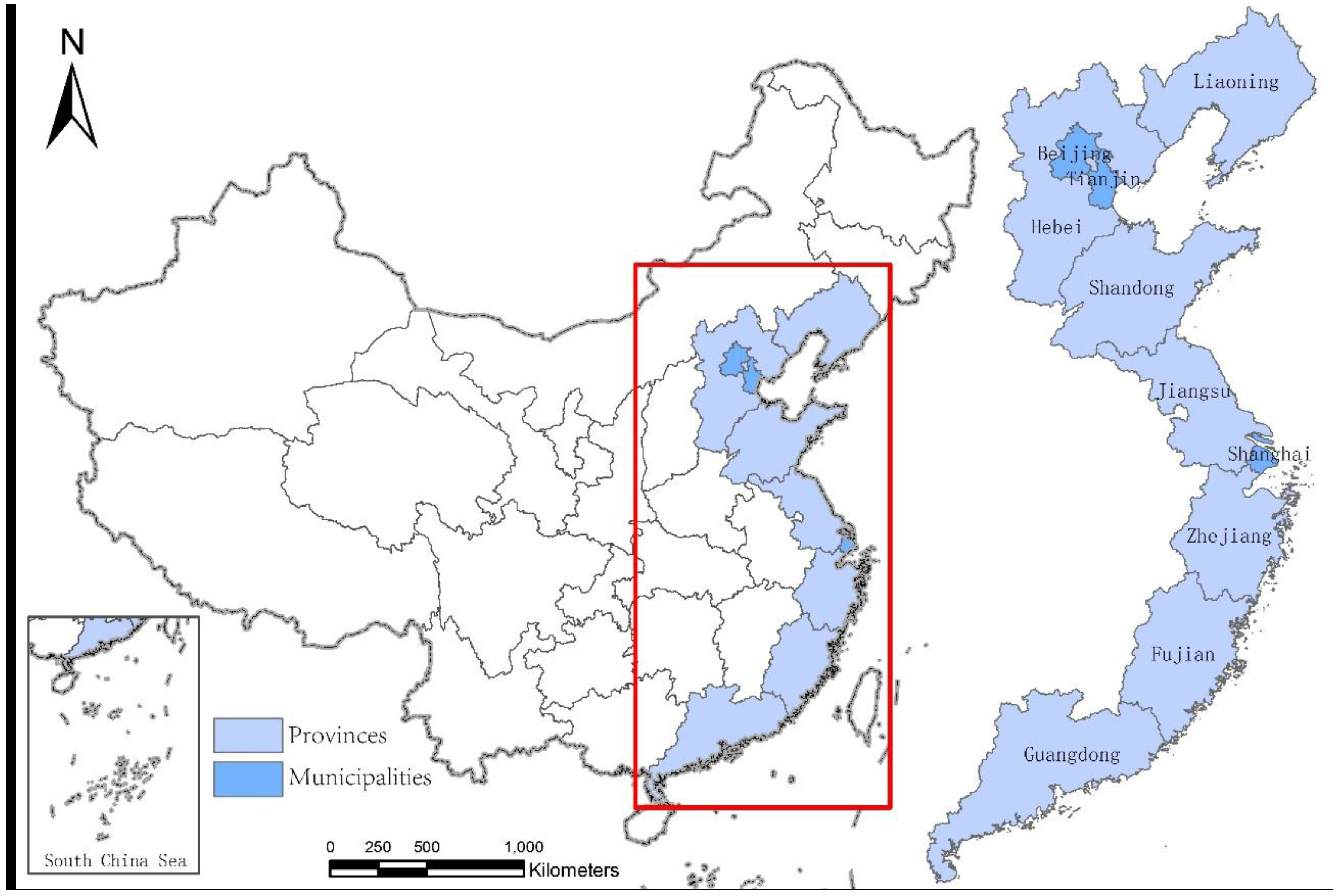
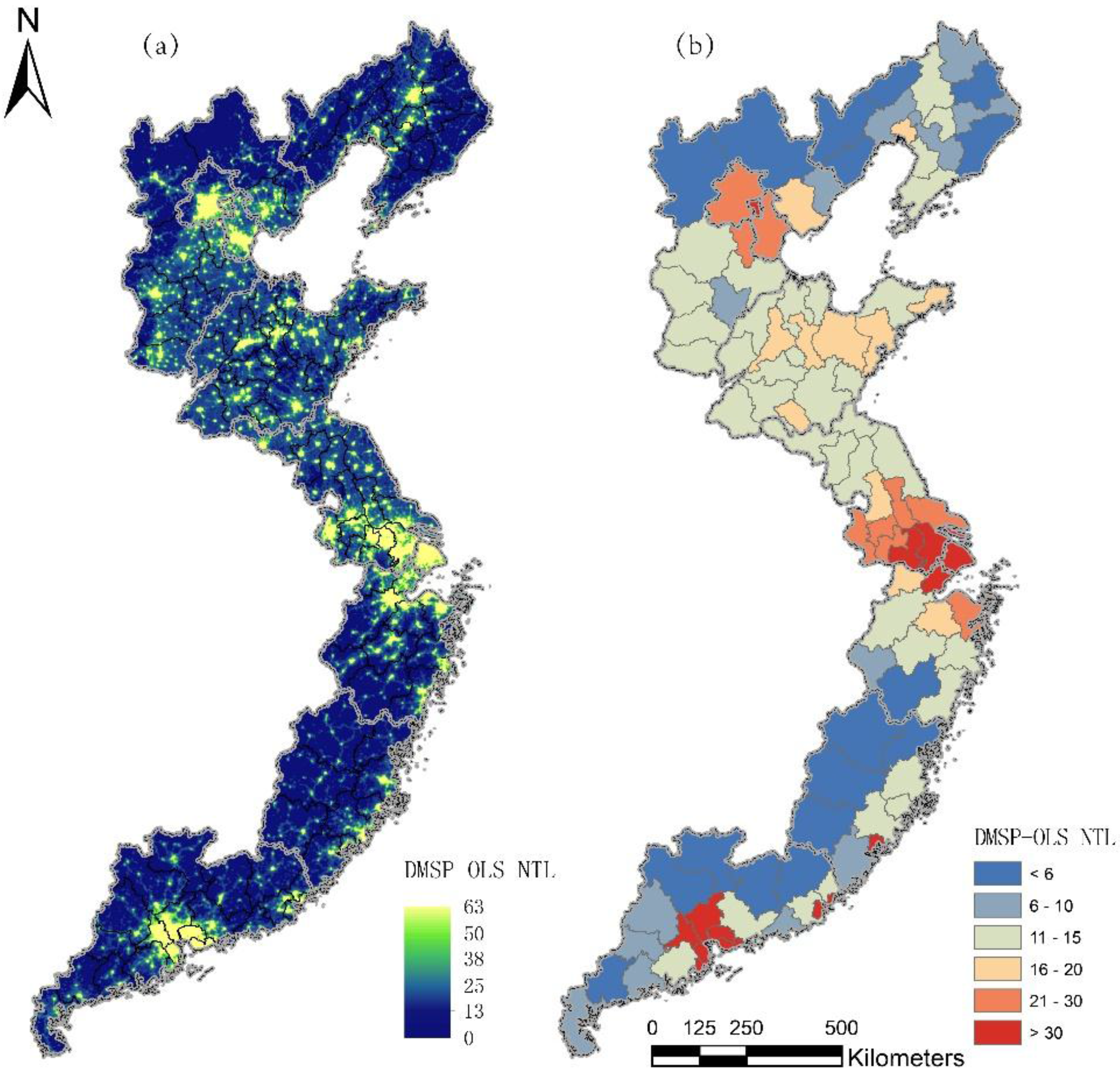
2. Study Area and Data Resources


| Abbreviation | Data Description | Spatial Resolution | Time |
|---|---|---|---|
| NTL | DMSP-OLS stable nighttime light | 1 km | 2010 |
| MOD13A3 | MODIS monthly NDVI | 1 km | 2010 |
| MOD44W | MODIS land water mask | 250 m | NA |
| FROM-GLC | Global land cover | 1 km | 2010 |
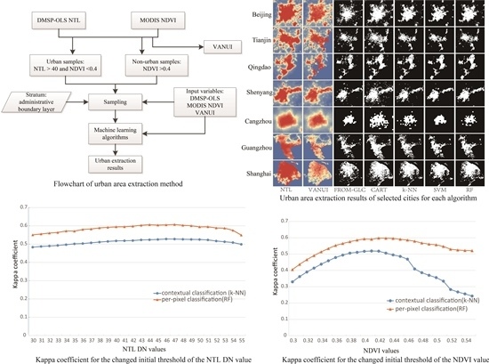
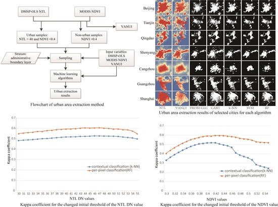
3. Methods

3.1. VANUI
3.2. Machine Learning Methods
| Classifiers | Abbreviation | Parameters | Remarks |
|---|---|---|---|
| Classification and Regression Tree | CART | Maximum depth: 50 | Data were scaled to [0,1] before training and classification |
| k-Nearest Neighbors | k-NN | Number of neighbors: 10 | |
| Support Vectors Machine | SVM | Kernel : RBF C(cost):1.0 gamma: 0.1 Probability estimates: false | |
| Random Forests | RF | Number of trees: 25 |
4. Results and Discussion
4.1. Performance of Machine Learning Methods
| Region | Training OA | Testing OA | ||||||
|---|---|---|---|---|---|---|---|---|
| CART | k-NN | SVM | RF | CART | k-NN | SVM | RF | |
| Beijing | 0.998 | - - | 0.95 | 0.987 | 0.909 | 0.97 | 0.96 | 0.939 |
| Tianjin | 0.997 | - - | 0.932 | 0.997 | 0.859 | 0.915 | 0.915 | 0.915 |
| Shanghai | 1 | - - | 0.874 | 0.986 | 0.769 | 0.821 | 0.821 | 0.744 |
| Hebei | 0.996 | - - | 0.988 | 0.993 | 0.982 | 0.986 | 0.983 | 0.986 |
| Liaoning | 0.992 | - - | 0.983 | 0.988 | 0.979 | 0.983 | 0.987 | 0.985 |
| Shandong | 0.986 | - - | 0.972 | 0.982 | 0.96 | 0.96 | 0.966 | 0.963 |
| Jiangsu | 0.988 | - - | 0.973 | 0.981 | 0.957 | 0.961 | 0.965 | 0.964 |
| Zhejiang | 0.989 | - - | 0.97 | 0.981 | 0.966 | 0.958 | 0.971 | 0.966 |
| Fujian | 0.999 | - - | 0.99 | 0.996 | 0.988 | 0.99 | 0.988 | 0.986 |
| Average | 0.994 | - - | 0.959 | 0.988 | 0.93 | 0.949 | 0.951 | 0.939 |
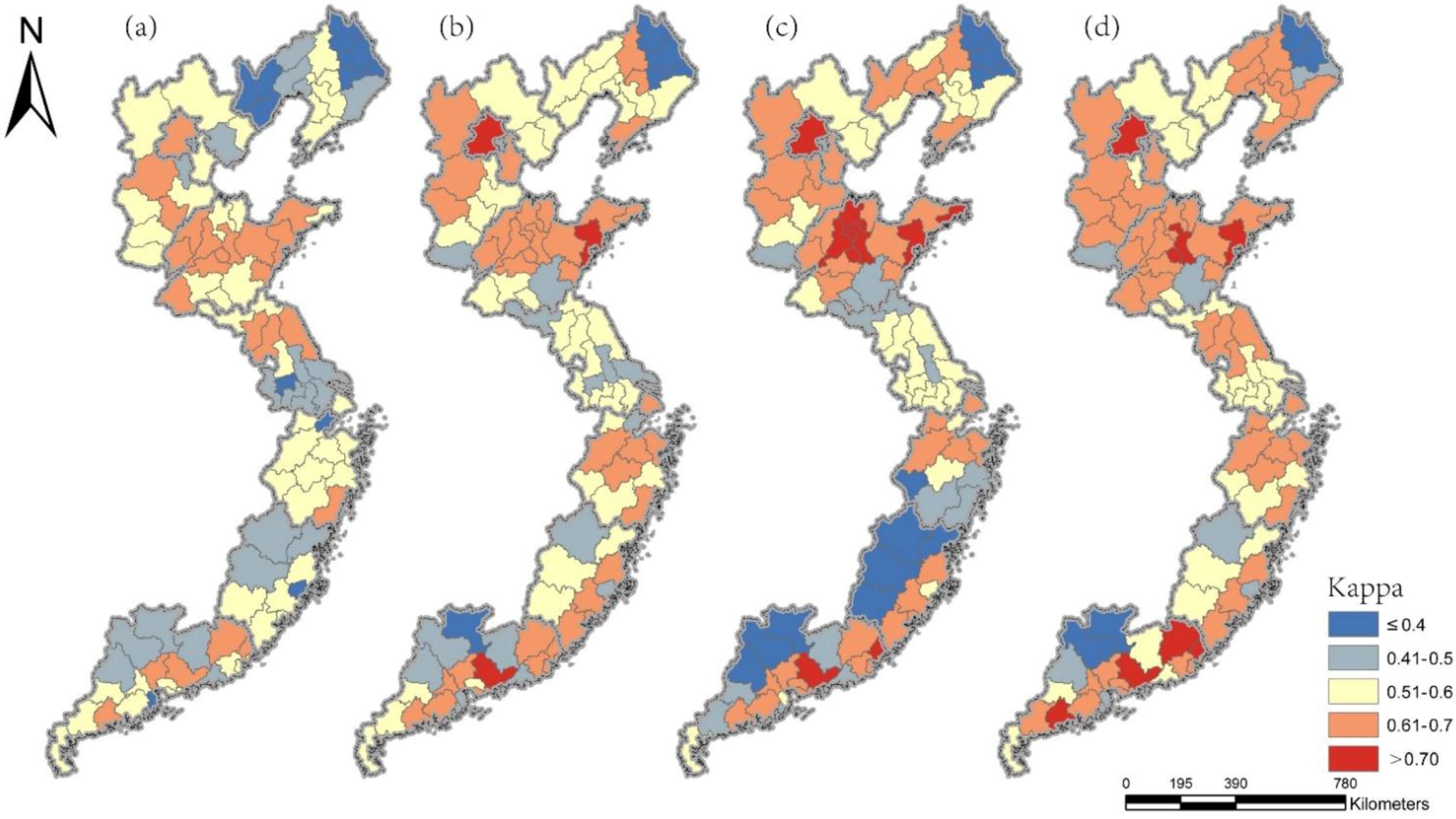
4.2. Mapping Urban Areas

| Province/Municipality | FROM-GLC Urban Pixels | CART | k-NN | SVM | RF | ||||||||
|---|---|---|---|---|---|---|---|---|---|---|---|---|---|
| OA | Kappa | Urban Pixels | OA | Kappa | Urban Pixels | OA | Kappa | Urban Pixels | OA | Kappa | Urban Pixels | ||
| Beijing | 2107 | 0.943 | 0.666 | 2892 | 0.961 | 0.727 | 2159 | 0.964 | 0.743 | 2000 | 0.96 | 0.733 | 2336 |
| Tianjin | 1323 | 0.907 | 0.54 | 2130 | 0.947 | 0.652 | 1293 | 0.956 | 0.696 | 1174 | 0.948 | 0.666 | 1407 |
| Shanghai | 2137 | 0.763 | 0.528 | 3222 | 0.836 | 0.649 | 2452 | 0.845 | 0.66 | 2257 | 0.832 | 0.642 | 2593 |
| Hebei | 296.4 | 0.964 | 0.527 | 518.9 | 0.978 | 0.569 | 258.6 | 0.981 | 0.588 | 194.1 | 0.979 | 0.593 | 242.8 |
| Shandong | 244.2 | 0.963 | 0.605 | 371.0 | 0.972 | 0.632 | 276.4 | 0.976 | 0.652 | 216.6 | 0.975 | 0.663 | 265.2 |
| Liaoning | 249.0 | 0.959 | 0.439 | 465.7 | 0.976 | 0.533 | 236.3 | 0.978 | 0.536 | 183.7 | 0.978 | 0.562 | 234.7 |
| Jiangsu | 302.1 | 0.941 | 0.509 | 513.9 | 0.959 | 0.53 | 312.9 | 0.967 | 0.548 | 215.5 | 0.962 | 0.571 | 313.0 |
| Zhejiang | 399.3 | 0.947 | 0.541 | 664.5 | 0.966 | 0.588 | 419.2 | 0.971 | 0.523 | 284.4 | 0.969 | 0.604 | 395.5 |
| Fujian | 199.8 | 0.964 | 0.517 | 365.5 | 0.978 | 0.6 | 221.1 | 0.981 | 0.555 | 160.0 | 0.979 | 0.611 | 231.3 |
| Guangdong | 408.2 | 0.903 | 0.522 | 643.0 | 0.929 | 0.557 | 484.1 | 0.939 | 0.535 | 408.2 | 0.933 | 0.571 | 459.5 |
| Average | 374.1 | 0.944 | 0.526 | 614.9 | 0.962 | 0.575 | 399.4 | 0.967 | 0.568 | 317.0 | 0.964 | 0.598 | 392.7 |


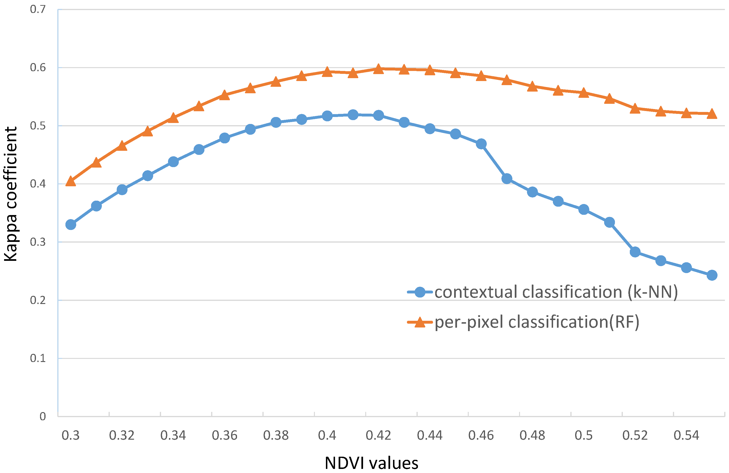
4.3. Comparison with the Contextual Classification
| CityProvince | FROM-GLC Urban Pixels | CART | k-NN | SVM | RF | ||||||||
|---|---|---|---|---|---|---|---|---|---|---|---|---|---|
| OA | Kappa | Urban Pixels | OA | Kappa | Urban Pixels | OA | Kappa | Urban Pixels | OA | Kappa | Urban Pixels | ||
| Beijing | 2107 | 0.859 | 0.450 | 2686 | 0.901 | 0.551 | 2029 | 0.863 | 0.463 | 2858 | 0.865 | 0.463 | 2636 |
| Tianjin | 1323 | 0.643 | 0.203 | 2234 | 0.779 | 0.339 | 2562 | 0.703 | 0.253 | 2493 | 0.699 | 0.248 | 2175 |
| Shanghai | 2137 | 0.859 | 0.641 | 1787 | 0.863 | 0.652 | 1794 | 0.866 | 0.670 | 2008 | 0.861 | 0.644 | 1784 |
| Hebei | 296.4 | 0.865 | 0.266 | 772.1 | 0.938 | 0.453 | 336.8 | 0.899 | 0.337 | 395.8 | 0.870 | 0.270 | 370.0 |
| Shandong | 244.2 | 0.948 | 0.539 | 339.2 | 0.962 | 0.612 | 323.5 | 0.953 | 0.568 | 330.6 | 0.948 | 0.539 | 339.0 |
| Liaoning | 249.0 | 0.905 | 0.286 | 435.3 | 0.958 | 0.459 | 286.7 | 0.941 | 0.382 | 349.6 | 0.907 | 0.289 | 319.3 |
| Jiangsu | 302.1 | 0.944 | 0.520 | 522.8 | 0.944 | 0.522 | 337.4 | 0.941 | 0.518 | 370.9 | 0.948 | 0.541 | 396.7 |
| Zhejiang | 399.3 | 0.960 | 0.515 | 247.1 | 0.961 | 0.528 | 254.1 | 0.962 | 0.545 | 274.1 | 0.961 | 0.519 | 244.9 |
| Fujian | 199.8 | 0.981 | 0.550 | 188.0 | 0.981 | 0.547 | 190.9 | 0.980 | 0.565 | 230.8 | 0.981 | 0.550 | 188.1 |
| Guangdong | 408.2 | 0.929 | 0.481 | 625.0 | 0.930 | 0.482 | 425.8 | 0.934 | 0.516 | 458.0 | 0.926 | 0.481 | 425.0 |
| Average | 374.1 | 0.928 | 0.451 | 509.4 | 0.948 | 0.514 | 428.6 | 0.939 | 0.491 | 505.1 | 0.929 | 0.456 | 449.6 |
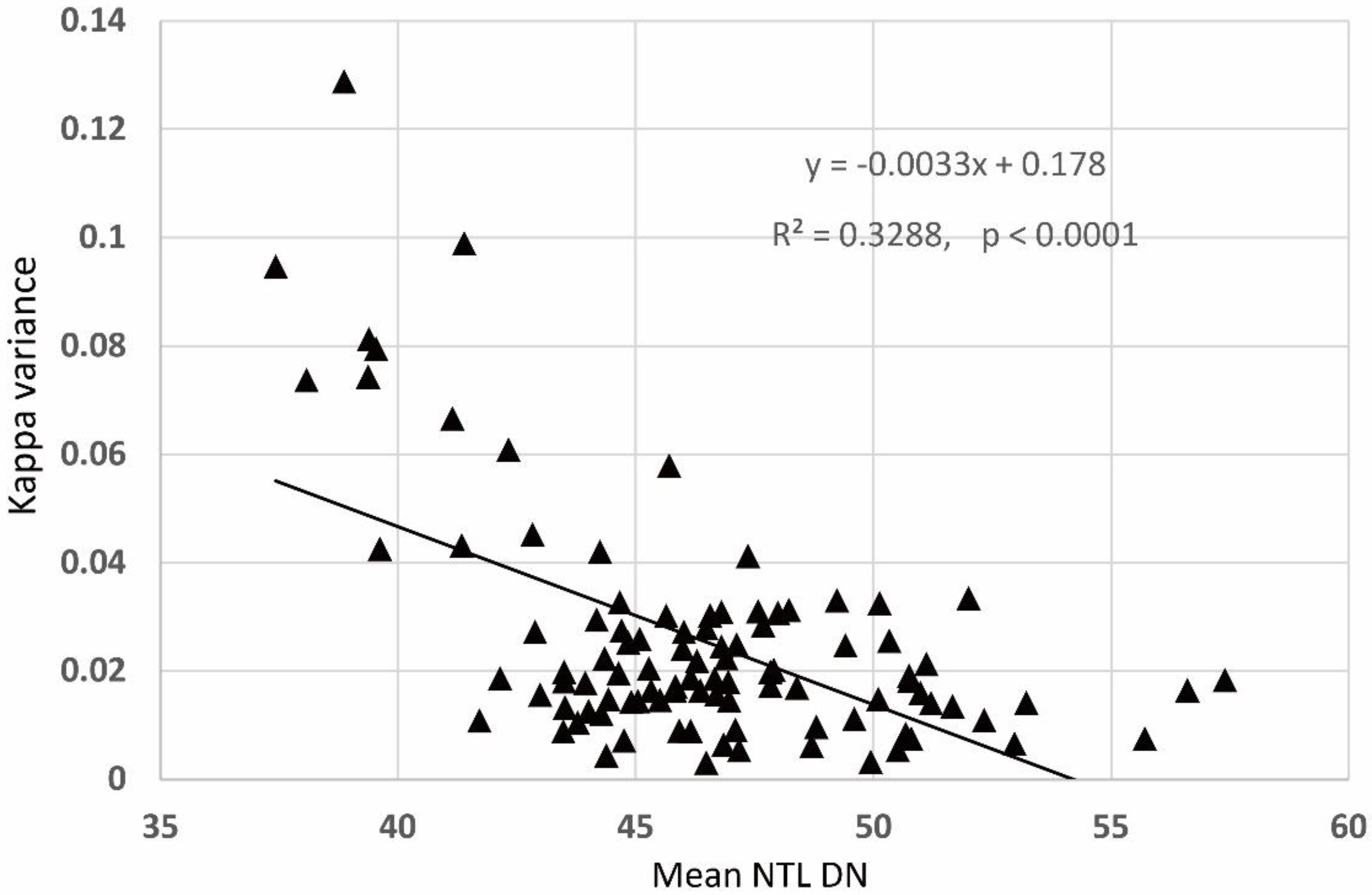
4.4. Sensitivity Analysis


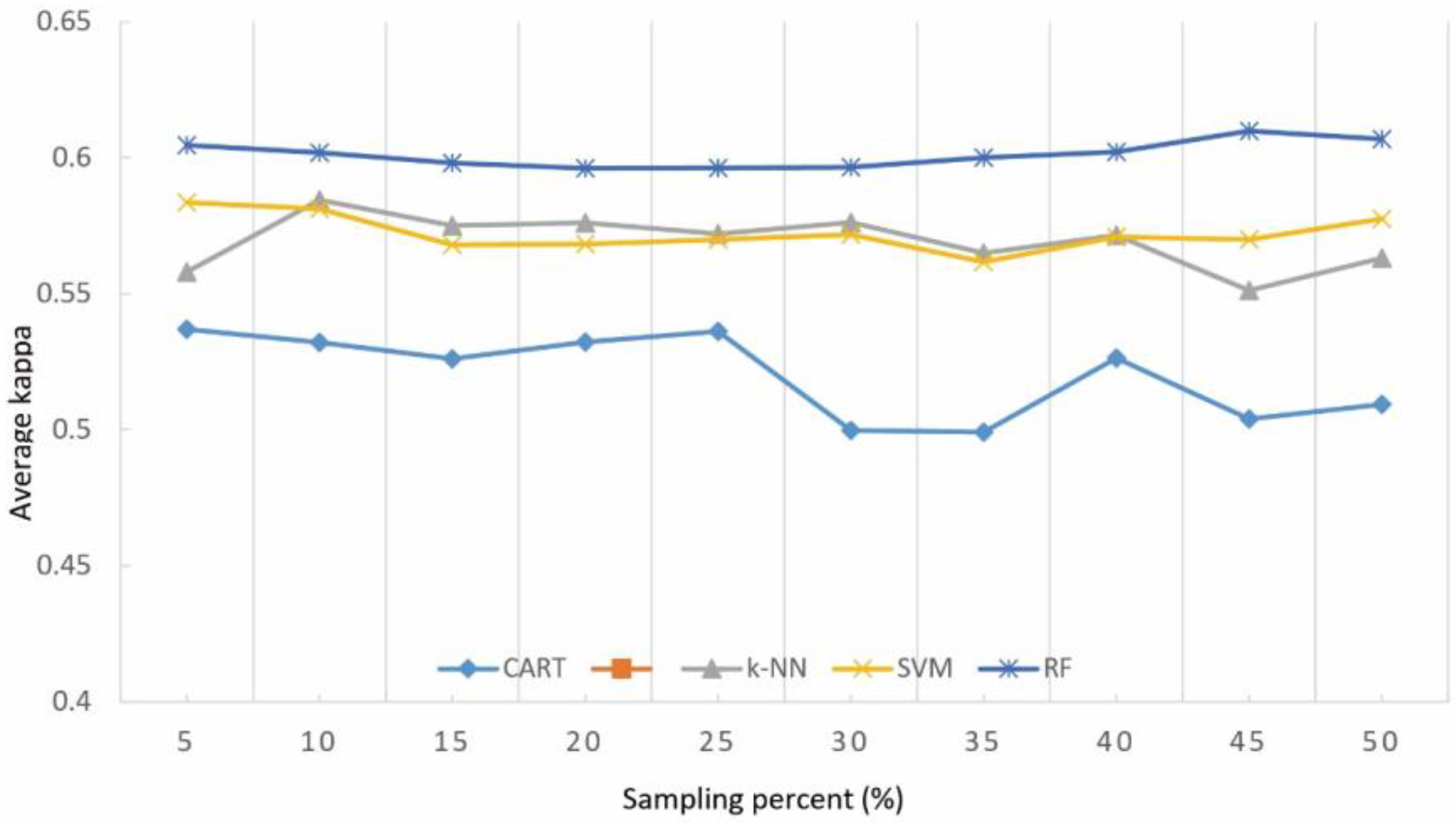
4.5. Impact of Different Training Set Percent
5. Discussion
6. Conclusions
Acknowledgments
Author Contributions
Conflicts of Interest
References
- Seto, K.C.; Fragkias, M.; Guneralp, B.; Reilly, M.K. A meta-analysis of global urban land expansion. PloS ONE 2011, 6, e23777. [Google Scholar] [CrossRef] [PubMed]
- Grimm, N.B.; Faeth, S.H.; Golubiewski, N.E.; Redman, C.L.; Wu, J.; Bai, X.; Briggs, J.M. Global change and the ecology of cities. Science 2008, 319, 756–760. [Google Scholar] [CrossRef] [PubMed]
- Foley, J.A.; DeFries, R.; Asner, G.P.; Barford, C.; Bonan, G.; Carpenter, S.R.; Chapin, F.S.; Coe, M.T.; Daily, G.C; Gibbs, H.K.; et al. Global consequences of land use. Science 2005, 309, 570–574. [Google Scholar]
- Hahs, A.K.; McDonnell, M.J.; McCarthy, M.A.; Vesk, P.A.; Corlett, R.T.; Norton, B.A.; Clemants, S.E.; Duncan, R.P.; Thompson, K.; Schwartz, M.W.; Williams, N.S.G. A global synthesis of plant extinction rates in urban areas. Ecol. Lett. 2009, 12, 1165–1173. [Google Scholar] [CrossRef] [PubMed]
- Seto, K.C.; Kaufmann, R.K.; Woodcock, C.E. Landsat reveals China’s farmland reserves, but they’re vanishing fast. Nat. 2000, 406, 121. [Google Scholar] [CrossRef] [PubMed]
- Rotem-Mindali, O.; Michael, Y.; Helman, D.; Lensky, I.M. The role of local land-use on the urban heat island effect of Tel Aviv as assessed from satellite remote sensing. Appl. Geogr. 2015, 56, 145–153. [Google Scholar] [CrossRef]
- Cao, X.; Chen, J.; Imura, H.; Higashi, O. A SVM-based method to extract urban areas from DMSP-OLS and SPOT VGT data. Remote Sens. Environ. 2009, 113, 2205–2209. [Google Scholar] [CrossRef]
- Li, C.; Li, C.; Wang, J.; Wang, L.; Hu, L.; Gong, P. Comparison of classification algorithms and training sample sizes in urban land classification with Landsat thematic mapper imagery. Remote Sens. 2014, 6, 964–983. [Google Scholar] [CrossRef]
- Lo, C.P.; Choi, J. A hybrid approach to urban land use/cover mapping using Landsat 7 enhanced thematic mapper plus (ETM+) images. Int. J. Remote Sens. 2004, 25, 2687–2700. [Google Scholar] [CrossRef]
- Lu, D.; Hetrick, S.; Moran, E. Land cover classification in a complex urban-rural landscape with QuickBird imagery. Photogramm. Eng. Remote Sens. 2010, 76, 1159–1168. [Google Scholar] [CrossRef]
- Myint, S.W.; Gober, P.; Brazel, A. Per-pixel vs. Object-based classification of urban land cover extraction using high spatial resolution imagery. Remote Sens. Environ. 2011, 115, 1145–1161. [Google Scholar]
- Weng, Q. Remote sensing of impervious surfaces in the urban areas: Requirements, methods, and trends. Remote Sens Environ. 2012, 117, 34–49. [Google Scholar]
- Zhang, Q.; Seto, K.C. Mapping urbanization dynamics at regional and global scales using multi-temporal DMSP/OLS nighttime light data. Remote Sens. Environ. 2011, 115, 2320–2329. [Google Scholar] [CrossRef]
- Zhang, Q.; Schaaf, C.; Seto, K.C. The vegetation adjusted NTL urban index: A new approach to reduce saturation and increase variation in nighttime luminosity. Remote Sens. Environ. 2013, 129, 32–41. [Google Scholar] [CrossRef]
- Small, C.; Pozzi, F.; Elvidge, C. Spatial analysis of global urban extent from DMSP-OLS night lights. Remote Sens. Environ. 2005, 96, 277–291. [Google Scholar] [CrossRef]
- Imhoff, M.L.; Lawrence, W.T.; Stutzer, D.C.; Elvidge, C.D. A technique for using composite DMSP/OLS “City Lights” satellite data to accurately map urban areas. Remote Sens. Environ. 1997, 61, 361–370. [Google Scholar] [CrossRef]
- Henderson, M.; Yeh, E.T.; Gong, P.; Elvidge, C.; Baugh, K. Validation of urban boundaries derived from global night-time satellite imagery. Int. J. Remote Sens. 2003, 16, 595–609. [Google Scholar] [CrossRef]
- Manuel Fernandez-Delgado, E.C.; Barro, S. Do we need hundreds of classifiers to solve real world classification problems. J. Mach. Learn. Res. 2014, 49, 3133–3181. [Google Scholar]
- Bureau, C.S. China Statistical Year Book 2010; China Statistics Press: Beijing, China, 2010. [Google Scholar]
- Yu, L.; Wang, J.; Li, X.; Li, C.; Zhao, Y.; Gong, P. A multi-resolution global land cover dataset through multisource data aggregation. Sci. China Earth Sci. 2014, 57, 2317–2329. [Google Scholar] [CrossRef]
- Gong, P.; Wang, J.; Yu, L.; Zhao, Y.; Zhao, Y.; Liang, L; Niu, Z.; Huang, X; Fu, H.; Liu, S; et al. Finer resolution observation and monitoring of global land cover: First mapping results with Landsat TM and ETM+ data. Int. J. Remote Sens. 2013, 34, 2607–2654. [Google Scholar] [CrossRef]
- Yu, L.; Wang, J.; Gong, P. Improving 30m global land-cover map FROM-GLC with time series MODIS and auxiliary data sets: A segmentation-based approach. Int. J. Remote Sens. 2013, 34, 5851–5867. [Google Scholar] [CrossRef]
- Pandey, B.; Joshi, P.K.; Seto, K.C. Monitoring urbanization dynamics in India using DMSP/OLS night time lights and SPOT-VGT data. Int. J. Appl. Earth Obs. Geoinf. 2013, 23, 49–61. [Google Scholar] [CrossRef]
- Shao, Z.; Liu, C. The integrated use of DMSP-OLS nighttime light and MODIS data for monitoring large-scale impervious surface dynamics: A case study in the Yangtze River Delta. Remote Sens. 2014, 6, 9359–9378. [Google Scholar] [CrossRef]
- Rokach, L.; Maimon, O. Data Mining with Decision Trees: Theory and Applications; World Scientific Pub Co Inc: Singapore, 2008. [Google Scholar]
- Breiman, L.; Freidman, J.; Olshen, R.A.; Stone, C.J. Classification and Regression Trees (Wadsworth Statistics/Probability); Chapman and Hall/CRC: Boca Raton, FL, USA, 1984. [Google Scholar]
- Hand, D.; Mannila, H.; Smyth, P. Principles of Data Mining; The MIT Press: Cambridge, MA, USA, 2001. [Google Scholar]
- Altman, N.S. An introduction to kernel and nearest-neighbor nonparametric regression. Am. Stat. 1992, 46, 175–185. [Google Scholar]
- Harrington, P. Machine Learning in Action; Manning Publications: Shelter Island, NY, USA, 2012. [Google Scholar]
- Brian, S.; Everitt, S.L.; Leese, M.; Stahl, D. Miscellaneous Clustering Methods, in Cluster Analysis, 5 ed.; John Wiley & Sons, Ltd: Chichester, UK, 2011. [Google Scholar]
- Kotsiantis, S.B. Supervised machine learning—A review of classification techniques. Informatica 2007, 31, 249–268. [Google Scholar]
- Fabian Pedregosa, G.V.; Gramfort, A.; Michel, V.; Thirion, B.; Grisel, V.; Blondel, M.; Peter Prettenhofer, R.W.; Dubourg, V.; Vanderplas, J.; Passos, A.; et al. Scikit-learn: Machine learning in Python. J. Mach. Learn. Res. 2011, 12, 2825–2830. [Google Scholar]
- Breiman, L. Random forests. Mach. Learn 2001, 45, 5–32. [Google Scholar] [CrossRef]
- Fan, J.; Ma, T.; Zhou, C.; Zhou, Y.; Xu, T. Comparative estimation of urban development in China’s cities using socioeconomic and DMSP/OLS night light data. Remote Sens. 2014, 6, 7840–7856. [Google Scholar] [CrossRef]
- Lu, D.; Tian, H.; Zhou, G.; Ge, H. Regional mapping of human settlements in southeastern China with multisensor remotely sensed data. Remote Sens. Environ. 2008, 112, 3668–3679. [Google Scholar] [CrossRef]
- Ma, T.; Zhou, C.; Pei, T.; Haynie, S.; Fan, J. Quantitative estimation of urbanization dynamics using time series of DMSP/OLS nighttime light data: A comparative case study from China’s cities. Remote Sens. Environ. 2012, 124, 99–107. [Google Scholar] [CrossRef]
- Small, C.; Elvidge, C.D. Mapping decadal change in anthropogenic night light. Procedia Environ. Sci. 2011, 7, 353–358. [Google Scholar] [CrossRef]
- Li, X.; Xu, H.; Chen, X.; Li, C. Potential of NPP-VIIRS nighttime light imagery for modeling the regional economy of China. Remote Sens. 2013, 5, 3057–3081. [Google Scholar] [CrossRef]
© 2015 by the authors; licensee MDPI, Basel, Switzerland. This article is an open access article distributed under the terms and conditions of the Creative Commons Attribution license (http://creativecommons.org/licenses/by/4.0/).
Share and Cite
Jing, W.; Yang, Y.; Yue, X.; Zhao, X. Mapping Urban Areas with Integration of DMSP/OLS Nighttime Light and MODIS Data Using Machine Learning Techniques. Remote Sens. 2015, 7, 12419-12439. https://doi.org/10.3390/rs70912419
Jing W, Yang Y, Yue X, Zhao X. Mapping Urban Areas with Integration of DMSP/OLS Nighttime Light and MODIS Data Using Machine Learning Techniques. Remote Sensing. 2015; 7(9):12419-12439. https://doi.org/10.3390/rs70912419
Chicago/Turabian StyleJing, Wenlong, Yaping Yang, Xiafang Yue, and Xiaodan Zhao. 2015. "Mapping Urban Areas with Integration of DMSP/OLS Nighttime Light and MODIS Data Using Machine Learning Techniques" Remote Sensing 7, no. 9: 12419-12439. https://doi.org/10.3390/rs70912419