A Temperature and Emissivity Separation Algorithm for Landsat-8 Thermal Infrared Sensor Data

Abstract

On-board the Landsat-8 satellite, the Thermal Infrared Sensor (TIRS), which has two adjacent thermal channels centered roughly at 10.9 and 12.0 μm, has a great benefit for the land surface temperature (LST) retrieval. The single-channel algorithm (SC) and split-window algorithm (SW) have been applied to retrieve the LST from TIRS data, which need the land surface emissivity (LSE) as prior knowledge. Due to the big challenge of determining the LSE, this study develops a temperature and emissivity separation algorithm which can simultaneously retrieve the LST and LSE. Based on the laboratory emissivity spectrum data, the minimum-maximum emissivity difference module (MMD module) for TIRS data is developed. Then, an emissivity log difference method (ELD method) is developed to maintain the emissivity spectrum shape in the iterative process, which is based on the modified Wien’s approximation. Simulation results show that the root-mean-square-errors (RMSEs) are below 0.7 K for the LST and below 0.015 for the LSE. Based on the SURFRAD ground measurements, further evaluation demonstrates that the average absolute error of the LST is about 1.7 K, which indicated that the algorithm is capable of retrieving the LST and LSE simultaneously from TIRS data with fairly good results.

1. Introduction

As the result of all surface–atmosphere interactions, land surface temperature (LST) is often regarded as an indicator of the equilibrium thermodynamic state and the driving force of long-wave radiation exchange. Therefore, the LST is especially important for lots of studies, including climate change, evapotranspiration evaluation, hydrologic cycle, urban heat island, vegetation monitoring and environmental studies [1,2,3,4,5,6,7,8,9,10]. Additionally, the land surface emissivity (LSE) is also an important factor of the thermally emitted radiance from the surface, which depends on the material composition, surface roughness, wavelength, viewing angle and moisture [11,12,13,14].

Due to the complexity of the land surface, ground measurements cannot provide realistic large-scale and continuous LST and LSE information. However, the developments of remote sensing technology offer an effective approach to retrieve the LST and LSE over large spatial and temporal scales. Numerous studies have been conducted to retrieve the LST from the Advanced Very High Resolution Radiometer (AVHRR), Moderate Resolution Imaging Spectroradiometer (MODIS), Advanced Spaceborne Thermal Emission and Reflection Radiometer (ASTER) and Landsat Thematic Mapper (TM)/Enhanced Thematic Mapper Plus (ETM+) data. Meanwhile, a variety of algorithms have been developed, such as single-channel methods, split-window methods, multi-angle methods, physics-based day/night methods, two-temperature methods, artificial neural network methods, temperatures and emissivity separation methods, etc. [15,16,17,18,19,20,21,22,23,24].

Landsat-8 (also known as the Landsat Data Continuity Mission, LDCM) was successfully launched in February 2013, which extends the Landsat archives with high spatial resolution remote sensing data of a global coverage. Landsat-8 carries two instruments, i.e., the Operational Land Imager (OLI) and Thermal Infrared Sensor (TIRS). Among them, TIRS measures the thermal radiation at 100 m spatial resolution, which can provide finer land surface information [25,26]. Moreover, TIRS has two infrared bands and narrower bandwidths, which is of great benefit to the LST and LSE inversion. The noise-equivalent delta temperature (NEΔT) of the two thermal infrared bands onboard Landsat-8 should be ≤0.4 K at 300 K (prelaunch values). Later studies demonstrate that the NEΔT at 300 K is approximately 0.05 K for both channels, which is better than the TM/ETM+ [27,28].

One objective of the Landsat-8 mission is to collect and archive moderate-resolution, thermal multispectral image data affording seasonal coverage of the global land mass for a period of no less than three years [25]. Retrieving the LST/LSE from Landsat-8 TIRS can ensure that the data are sufficiently consistent with data from the earlier Landsat missions. This will permit studies of climate change and environmental research over multi-decadal periods. Besides, there are plenty of LST/LSE products already, such as the LST/LSE products from MODIS and ASTER data. However, the spatial resolutions of the products are relatively low (MODIS products) or they are not free to users (ASTER products). The products from Landsat-8 TIRS could distribute data with moderate-resolution and at no cost to users.

Given TM/ETM+ only have one infrared band, the single-channel algorithm (SC) is the only method that can be applied to retrieve the LST. Based on the radiative transfer model (RTM), SC algorithms calculate the atmospheric attenuation and emitted radiance in a given band, and thus to obtain the LST from the surface emitted radiances. On the basis of the known LSE and water vapor content, several single-channel methods have been developed in the past decade, which are also suitable for Landsat-8 [16,29,30]. However, the LSE is rarely known and an uncertainty of 1% in the LSE would lead to an error in the LST ranges from 0.3 K to 0.7 K depending on the atmospheric condition [31]. Moreover, owing to the unstable empirical relationship, the SC algorithms provide poor results for high atmospheric water vapor content [32,33], including the Landsat-8 TIRS data [34].

Since the TIRS have two infrared bands, split-window algorithms (SW), which correct the atmospheric effects based on the differential absorption in two adjacent infrared bands, can be used to retrieve the LST. Several SW techniques have been developed for remote sensing data with two infrared bands, which have been successfully applied to the TIRS data [34,35,36,37]. The accuracy of the SW algorithms depend on the accuracy of parameters, including the LSE, the atmospheric water vapor content, air temperature and the coefficients. The coefficients are always calculated by statistical fit from a simulated database. Simulation tests show that the RMSE of different SW algorithms for TIRS data is about 1 K, on the assumption that the parameters have no errors [34,35]. However, a 1% error in LSE would result in about 1 K error of the LST, in particular for dry atmospheric conditions [35], and an extensive validation with in situ measurements needs to be conducted rather than with the simulated data.

On account of the high heterogeneity of the surface and the spectral variation of the LSE; it is a big challenge to determine the LSE when the satellite passes. As a result, the extensive application of SC and SW algorithms is limited. Up to now, a variety of methods have been demonstrated to estimate the LST when the LSE is unknown [13], including temperature-independent spectral-indices method (TISI); MODIS day/night method; ASTER temperature and emissivity separation method (TES) and Alpha derived emissivity method (ADE), etc. [15,19,38,39,40,41,42]. Based on the radiative transfer equation; a single multispectral measurement with N bands only presents N observations for N+1unknown parameters. Without any prior information, it is impossible to recover both LST and emissivities exactly. Many temperature and emissivity methods use one additional empirical equation so that N+1 unknowns can be solved by N+1 equations. However, because any added equations are based on empirical formula, the solutions are likely to be unstable. The inversion problem is called well posed if the solution exists, can be uniquely determined, and depends continually on the data [19]. Therefore, simultaneously retrieving the LST and the LSE is a typical ill-posed problem. Additional information is needed to turn it into a well posed problem. The MODIS day/night method solves the ill-posed problem by assuming the emissivity has no significant change between day and night [40]. The ASTER TES algorithm comprises of three modules: normalized emissivity method (NEM); mean maximum-minimum apparent emissivity difference method (MMD); and ratio algorithm. Based on the empirical relationship between the spectral contrast and the minimum emissivity, the MMD method provides an additional equation, and the ratio algorithm is used to keep the shape of the emissivity spectrum. Similarly, the ADE method introduces one equation depicting the empirical relationship between the mean and variance of Alpha spectra whose shape is almost the same as the emissivity.

Since the SC and SW methods need the prior knowledge of the LSE and the accuracy of the retrieved LST is primarily dependent on the accuracy of the LSE, simultaneous determination of the LSE and the LST by TES algorithms would be an alternative approach to retrieve the LST from TIRS data. Although previous studies demonstrate that the TES methods require at least four TIR bands and no studies have been conducted with only two TIR bands [43,44], this present paper would like to investigate the possibility of TES algorithm using the two TIR bands of TIRS. From the above description, there are two main issues concerning the temperature and emissivity separation algorithms: (1) provide one additional equation or other additional information; (2) recover the emissivity spectrum by keeping the form of the actual emissivity spectral curve. Consequently, an empirical relationship between the minimum emissivity and the minimum-maximum emissivity difference (MMD) is developed based on the laboratory spectral data. Besides, the ratio module is infeasible because TIRS only has two bands. Thus, the emissivity log difference method, which is based on the modified Wien’s approximation, is developed to maintain the shape of the emissivity spectral curve.

2. Data Sets

2.1. Simulation Data

Simulation data is obtained from the MODTRAN 5 radiative transfer code [45], which needs the atmospheric profiles, LSE and LST as inputs. The six model atmospheric profiles of MODTRAN are used as atmospheric profile inputs, and a total of 96 emissivity spectra (including vegetation, water, ice, snow, soil and rock) are used as LSE inputs in the simulation. For the LST inputs, according to the previous studies [34], the following individual values are considered for the LST: T₀ − 5, T₀, T₀ + 5, T₀ + 10 and T₀ + 20, where T₀ is the temperature at the lowest layer of the atmospheric profile. However, the highest temperature T₀ + 20 would be too low for some desert areas, thus T₀ + 30 is added for the simulation. The outputs consist of brightness temperature, atmospheric transmittance and atmospheric thermal radiance (upward and downward atmospheric thermal radiance), which are obtained by convolution between the MODTRAN spectral outputs and the TIRS spectral response functions.

2.2. Ground LST Measurements

In order to support climate research with long-term, continuous and accurate surface radiation measurements, SURFRAD was established for the United States in 1995 [46,47]. High-quality in situ measurements of upward and downward solar and infrared radiation are provided. The downwelling and upwelling radiation data are measured by a pyrgeometer which is deployed 10 m above the sea level, collecting a sample every minute in a spectral window from 3 to 50 μm. Four SURFRAD sites are selected in this study, as described in Table 1.

Table 1. Descriptions of the four SURFRAD sites.

Site	Lat/Lon	Elevation (km)	Land Cover
Bondville, Illinois	40.05N, 88.37W	0.213	Crop Land
Fort Peck, Montana	48.31N, 105.10W	0.634	Grass Land
Goodwin Creek, Mississippi	34.25N, 89.87W	0.098	Evergreen Needle Leaf Forest
Sioux Falls, South Dakota	43.73N, 96.62W	0.473	Rural Land

Table 1. Descriptions of the four SURFRAD sites.

Site	Lat/Lon	Elevation (km)	Land Cover
Bondville, Illinois	40.05N, 88.37W	0.213	Crop Land
Fort Peck, Montana	48.31N, 105.10W	0.634	Grass Land
Goodwin Creek, Mississippi	34.25N, 89.87W	0.098	Evergreen Needle Leaf Forest
Sioux Falls, South Dakota	43.73N, 96.62W	0.473	Rural Land

In this study, the upward and downward infrared radiations measured by SURFRAD are used for the evaluation of retrieved LST. According to the Stefan-Boltzmann law, the LST can be estimated from:

$$T_s={{\displaystyle \left[\frac{L_{\uparrow }-\left(1-{\text{ε}}_b\right)\cdot L_{\downarrow }}{{\text{ε}}_b\cdot \sigma }\right]}}^{1/4}$$

(1)

where L_↑ and L_↓ are the surface upwelling and downwelling longwave radiation, respectively, σ is the Stefan- Boltzmann’s constant (5.67 × 10⁻⁸ W∙m⁻²∙K⁴), and ${\text{ε}}_b$ is the broadband emissivity. The broadband emissivity can be estimated from MODIS narrowband emissivities in the thermal region [48]:

$${\text{ε}}_b=0.2122\cdot {\text{ε}}_{29}+0.3859\cdot {\text{ε}}_{31}+0.4029\cdot {\text{ε}}_{32}$$

(2)

where ${\text{ε}}_{29}$, ${\text{ε}}_{31}$ and ${\text{ε}}_{32}$ are narrowband emissivities of MODIS band 29, 31 and 32, respectively.

The accuracy of the LST estimated from Equation (1) depends on the accuracy of the upward and downward radiation and the satellite broadband emissivity measurements. The accuracy of the pyrgeometer is measured as about 9 W∙m⁻² [46], and the study using the same type of pyrgeometers shows that the error is about 3–5 W∙m⁻², equivalent to an error of 0.5–0.8 °C in the LST [49]. The accuracy of the LST also depends on the broadband emissivity retrieval. Comparison results with ground measurements demonstrate that accuracy of broadband emissivity by Equation (2) is about 0.0085 [48]. Moreover, the sensitivity of LST to broadband emissivity is about 0.10K/0.01 to 0.35K/0.01, which means that the accuracy of the LST is about 0.1–0.4K when the error of broadband emissivity is about ±0.01 [49]. The L_↑ is measured in the 10 m tower. At night, when there is a temperature inversion and the air at the 10 m elevation is warmer than at the surface, the measured L_↑ will be greater than the actual L_↑. Thus, the LST obtained from Equation (1) would be greater than the actual LST during nighttime, with an error of about 0–0.3 °C, while the conditions are just the opposite during the daytime [49].

2.3. Landsat-8 TIRS Data

In this study, 40 Landsat-8 TIRS images during 2013–2014 were downloaded from the United States Geological Survey (USGS) Earth-Explorer Website, corresponding to the four SURFRAD sites. Owing to the stray light, the USGS has reported a calibration problem of TIRS bands (http://landsat.usgs.gov/mission_headlines2014.php). Therefore, the reprocessed data after 3 February 2014 were ordered to avoid the problem. Following the guidelines at the USGS website, the digital number (DN) is converted to radiance and brightness temperature with the calibration parameters directly accessed from the metadata file. In order to avoid the influence of the clouds, a cloud mask is generated based on band 9 (the cirrus band) and band 11 (the quality band) (http://landsat.usgs.gov/L8QualityAssessmentBand.php).

2.4. Atmospheric Profiles

Atmospheric profiles are obtained from ground-based radiosoundings, numerical weather prediction (NWP) models or satellite vertical sounders. If actual radiosonde balloons are launched near the same area when the satellite passes over, ground-based radiosoundings can provide the most accurate description of the atmospheric state coincident with the satellite measurements spatially and temporally. However, due to insufficient spatial density of the ground-based radiosoundings, they are more suitable for validation at some certain sites rather than as a globally applicable algorithm [13]. On the contrary, atmospheric profiles provided by satellite vertical sounders can be used to retrieve the LST globally. In particular, Aqua AIRS is a high spectral resolution sounder with 2378 bands between 3.7 and 15 μm, providing atmospheric profiles with 45 km spatial resolution. Additionally, the MOD07 L2 atmospheric profiles with spatial resolution of 5 km from MODIS Terra also can be used to retrieve the LST, although their accuracy is lower than AIRS. Moreover, the air temperatures of MOD07 L2 profiles are consistently 1 K larger than that of AIRS, which would result in a slight overestimation of the ground LST by the single-channel algorithm [50]. Nevertheless, the observation time of the Terra/Aqua and Landsat-8 satellites are not the same over the entire world. The effect of the temporal gap might be significant for retrieving the LST.

In addition to the radiosonde and satellite sounded atmospheric profiles, meteorological forecasting models constitute an alternative source of the atmospheric profiles, such as the National Centers for Environmental Prediction (NCEP). As the reanalysis result of the radiosoundings data, ground measurements and satellite measurements, the NCEP reanalysis product provides 1°×1° resolution atmospheric profiles every 6 h globally [51]. The data are provided in 26 mandatory pressure levels from 1000 to 10 hPa, and consist of eastward and northward wind components, geopotential height, the air temperature and the relative humidity. The on-line atmospheric correction tool is used to extract the profile [52], which spatially interpolates the profiles to the sites and then temporally interpolates them to the observation time of the satellite. Benefitting from global coverage and high temporal resolution, the NCEP atmospheric profiles have been widely used for a variety of studies, which demonstrate that they can yield reasonable results to meet the required accuracy [50,53]. Therefore, the atmospheric profiles provided by NCEP reanalysis data are used to retrieve the LST in this study.

3. Experimental Section

An infrared sensor viewing the earth’s surface measures thermal radiation from the ground and the atmosphere along the line of sight. Since the ground is not a blackbody, the land surface emissivity has to be considered for calculating the emitted radiation of the ground. The atmosphere plays an important role in the transfer of the radiation from the surface propagating to the height of the satellite. Under the presumption of a cloud-free sky, the channel infrared radiance L_i at the top of the atmosphere (TOA) can be formulated as:

$$L_i={\tau }_i\left[{\text{ε}}_i{B}_i\left(T_s\right)+\left(1-{\text{ε}}_i\right)L_{ati\downarrow }+\left(1-{\text{ε}}_i\right)L_{si\downarrow }+{\rho }_{bi}{E}_i\cos \left({\text{θ}}_s\right){\tau }_i\left({\text{θ}}_s\right)\right]+L_{ati\uparrow }+L_{si\uparrow }$$

(3)

where ${\tau }_i$ is the effective transmittance of the atmosphere in channel i, ${\text{ε}}_i$ is the effective emissivity of the land surface in channel i, T_s is the LST, L_ati↑ and L_ati↓ are the upwelling and downwelling atmospheric radiance, respectively, L_ati↑ and L_ati↓ are the upward and downward solar diffuse radiance, respectively, ${\rho }_{bi}$ is the bi-directional reflectivity of the surface, Ei is the solar irradiance along solar zenith angle ${\theta }_s$ at the TOA. As the contribution of solar radiation in the infrared bands (8–14 μm) is negligible during day and night, the solar related items in Equation (3) can be neglected, thus the equation can be simplified as:

$$L_i={\tau }_i\left[{\text{ε}}_i{B}_i\left(T_s\right)+\left(1-{\text{ε}}_i\right)L_{ati\downarrow }\right]+L_{ati\uparrow }$$

(4)

On the basis of known atmospheric profiles, upwelling and downwelling atmospheric radiance and atmospheric transmittance can be calculated by MODTRAN. As discussed in Section 1, without any prior information of the LSEs, additional information is needed to solve the ill-posed problem by temperature and emissivity separation algorithms, which is presented in the following part. Besides, while calculating the LST, the form of the actual emissivity spectral curve has to be maintained by a certain method, which is also presented in this section.

3.1. MMD Module for TIRS Data

In order to solve the ill-posed retrieval problem, a variety of methods have been developed, including the TISI method, day/night method, ADE method and MMD method. The day/night algorithm doubles the number of measurements by assuming the LSE has no significant change between day and night, which suffers from the critical problem of geometry mis-registration and variation in the VZA (viewing zenith angle). By utilizing an empirical relationship between the standard deviation and mean emissivity of multiple observations, the ADE method can restore the amplitude of the emissivity. However, the use of Wien’s approximation will introduce large emissivity error, and at least three infrared bands are needed to fit the empirical relationship. Based on the laboratory emissivity spectrum data, the MMD method calculates the minimum LSE by the empirical relationship between the minimum LSE and the spectral contrast in N channels. Owing to the advantages of the MMD method, it is utilized in this study to separate the temperature and emissivity of Landsat-8 TIRS data.

The MMD method is established by the laboratory emissivity spectrum data, which is obtained from the ASTER spectral library (version 2.0, available on CD-ROM or on-line at http://speclib.jpl.nasa.gov). The library is a collection of contributions in a standard format from the Jet Propulsion Laboratory (JPL), Johns Hopkins University (JHU) and USGS. A comprehensive collection of over 2300 spectra of a wide variety of materials covering the wavelength ranges from 0.4 to 15.4 μm is provided in the dataset [54]. In total, 96 laboratory emissivity spectra of natural surfaces (including vegetation, water, snow, ice, soils and rock) are utilized in this study. Individual emissivity spectra are deduced from Kirchhoff’s law. Following the previous study [55], because they may not follow Kirchhoff’s law, the spectra of fine powdered samples (particle size smaller than 75 μm for the JHU library or smaller than 45 μm for the JPL library) are eliminated.

Since the LSE varies with the wavelength, the effective emissivity in channel j for a given wavelength ranging from ${\text{λ}}_1$ to ${\text{λ}}_2$ can be calculated by:

$${\text{ε}}_j=\frac{{\displaystyle {\int }_{{\lambda }_1}^{{\lambda }_2}{f}_j\left(\lambda \right)\cdot \text{ε}\left(\lambda \right)\cdot d\lambda }}{{\displaystyle {\int }_{{\lambda }_1}^{{\lambda }_2}{f}_j\left(\lambda \right)\cdot d\lambda }},j=10,11$$

(5)

where $f_i\left(\text{λ}\right)$ is the sensor’s normalized spectral response function for channel j, which satisfies ${{\displaystyle \int }}_{{\text{λ}}_1}^{{\text{λ}}_2}{f}_i\left(\text{λ}\right)d\text{λ}=1$.

After obtaining the effective emissivity of the 96 laboratory emissivity spectra, the relative emissivity can be calculated from the following equation:

$${\text{β}}_j=2\cdot {\text{ε}}_j\cdot {\left[{\displaystyle \sum {\text{ε}}_j}\right]}^{-1},j=10,11$$

(6)

where ${\text{β}}_j$ is the relative emissivity of band j. Then, the spectral contrast, namely the maximum and minimum relative emissivity difference (MMD), is determined by:

$$MMD=\max \left({\text{β}}_j\right)-\mathrm{mix}\left({\text{β}}_j\right)$$

(7)

The relationship between the minimum LSE and the MMD is fitted and the equation can be formulated as:

$${\text{ε}}_{\min }=0.983-1.027\cdot MM{D}^{0.861},{\text{R}}^2=0.945$$

(8)

The empirical relationship between the ${\text{ε}}_{min}$ and MMD is presented in Figure 1. Four types of vegetation, six types of water/ice/snow, 52 types of soils and 34 types of rocks are included in this study. The average absolute error, the RMSE and the regression coefficient (R) are about 0.006, 0.010 and 0.972, respectively. As shown in [19], the squared correlation coefficient of ASTER MMD algorithm is 0.983, which is a bit better than the MMD method of TIRS. The main difference between them is that Landsat-8 only has two infrared bands while ASTER has five infrared bands. With the empirical equation, the LST/LSE can be determined, although the empirical equation has some error which cannot be eliminated. Nevertheless, based on the maintenance of the emissivity spectral shape by a certain method, the LSEs of the TIRS bands can be calculated precisely after a few iterations, and thus the LST can be derived accordingly.

Figure 1. The empirical relationship between the ${\text{ε}}_{min}$ and MMD of Landsat-8 TIRS data. R is the regression coefficient, RMSE is the root mean square error and n is the number of surface types.

Figure 1. The empirical relationship between the ${\text{ε}}_{min}$ and MMD of Landsat-8 TIRS data. R is the regression coefficient, RMSE is the root mean square error and n is the number of surface types.

3.2. Maintenance of the Emissivity Spectral Shape

Based on the MMD module, additional information is added to make the ill-posed problem solved, yet the MMD method may have some error. To increase the accuracy of the temperature and emissivity algorithm, an iterative process is always needed to maintain the emissivity spectral shape by a certain method. The ASTER TES algorithm keeps the emissivity spectral shape through the ratio algorithm. Nevertheless, more than three infrared bands are needed to use the ratio algorithm [13,19]. The ADE method defines an alpha-residual spectrum based on the Wien’s approximation, which maintains the shape of the emissivity spectrum and can be applied to satellite data with only two infrared bands, such as the TIRS [41]. Therefore, an emissivity log difference method is developed in this study to maintain the emissivity spectrum shape, which is based on the modified Wien’s approximation.

As shown in the previous part, the channel radiance L_i at the top of the atmosphere (TOA) can be expressed as Equation (4). In Equation (4), the B_i(T_s) term is the radiance of a blackbody at land surface temperature T_s:

$$B_j\left(T_s\right)=\frac{C_1}{{\lambda }_j^5\cdot \pi \cdot \left(e^{C_2/{\lambda }_j{T}_s-1}\right)}$$

(9)

where $C_1=2\pi h{c}^2$ is the first radiation constant, $C_2=hc/k$ is the second radiation constant, h is Planck’s constant, c is the speed of light, k is Boltzmann’s constant and ${\text{λ}}_j$ is the wavelength of band j. Wien’s approximation neglects the −1 term in Equation (9), which will introduce slope errors into the emissivity spectrum. In this study, an adjustment item is added to modify the Wien’s approximation:

$$B_j\left(T_s\right)=\frac{C_1}{{\lambda }_j^5\cdot \pi \cdot e^{C_2/{\lambda }_j{T}_s}}\cdot N_j\left(T_s\right)$$

(10)

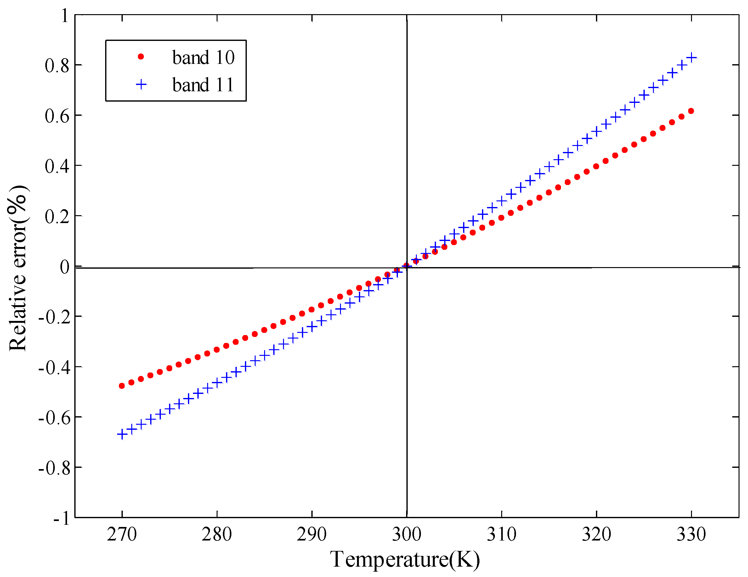
where $N_j\left(T_s\right)=1/\left(1-e^{-C_2/{\text{λ}}_j{T}_s}\right)$ is the adjustment item of band j, which is only affected by the LST. Moreover, in order to separate the emissivity and the temperature, the adjustment item has to be known. Thus, the sensitivity of the adjustment item to temperature has been conducted in TIRS band 10 and band 11 at 300 K, as seen in Figure 2. This result shows that the adjustment item changes about 0.2%–0.3% every 10 K, and that the largest relative errors of the adjustment item are about 0.62% and 0.83% for band 10 and 11, respectively, when the temperature gap is 30 K. Therefore, the adjustment item is not strongly sensitive to the variation of temperature. T_s can be replaced by the brightness temperature of band j(T_j), whose gap with the T_s would not exceed 30 K under normal circumstances. The modified Wien’s approximation can be expressed as:

$$B_j\left(T_s\right)\approx \frac{C_1}{{\lambda }_j^5\cdot \pi \cdot e^{C_2/{\lambda }_j{T}_s}}\cdot N_j\left(T_j\right)$$

(11)

Based on the simulation data by the MODTRAN model presented in Section 2, the comparisons between the Wien’s approximation and the modified Wien’s approximation are shown in Table 2. From Table 2 we can see that Wien’s approximation would lead to about 1%–2.5% underestimation of the blackbody radiance, which will bring slope error into the emissivity shape. The modified Wien’s approximation yields better results with about 0.20% relative error on average, although there is still a slight underestimation.

Figure 2. The relative error of the adjustment item which takes 300 K as a reference ($\frac{N_j\left(T_j\right)-N_j\left(300\right)}{N_j\left(300\right)}$).

Figure 2. The relative error of the adjustment item which takes 300 K as a reference ($\frac{N_j\left(T_j\right)-N_j\left(300\right)}{N_j\left(300\right)}$).

Table 2. Comparisons between the Wien’s approximation and the modified Wien’s approximation.

Temperature	Relative Error between the Approximation and the True Value of Bj(Ts) (%) (2)
	Wien’s Approximation	Modified Wien’s Approximation
T0 (3) − 5	−1.04/−1.59 (1)	−0.04/−0.06
T0	−1.13/−1.70	−0.07/−0.11
T0 + 5	−1.21/−1.82	−0.10/−0.17
T0 + 10	−1.30/−1.95	−0.13/−0.23
T0 + 20	−1.50/−2.21	−0.21/−0.36
T0 + 30	−1.71/−2.48	−0.28/−0.49

Note: ⁽¹⁾ For an example, −1.04/−1.59 means that the relative errors are about −1.04% for band 10 and −1.59% for band 11, respectively; ⁽²⁾ The relative error based on the Modified Wien’s approximation is the average value of simulation data from 96 laboratory emissivity spectra; ⁽³⁾ T₀ is the temperature at the first layer of the atmospheric profile.

Table 2. Comparisons between the Wien’s approximation and the modified Wien’s approximation.

Temperature	Relative Error between the Approximation and the True Value of Bj(Ts) (%) (2)
	Wien’s Approximation	Modified Wien’s Approximation
T0 (3) − 5	−1.04/−1.59 (1)	−0.04/−0.06
T0	−1.13/−1.70	−0.07/−0.11
T0 + 5	−1.21/−1.82	−0.10/−0.17
T0 + 10	−1.30/−1.95	−0.13/−0.23
T0 + 20	−1.50/−2.21	−0.21/−0.36
T0 + 30	−1.71/−2.48	−0.28/−0.49

Note: ⁽¹⁾ For an example, −1.04/−1.59 means that the relative errors are about −1.04% for band 10 and −1.59% for band 11, respectively; ⁽²⁾ The relative error based on the Modified Wien’s approximation is the average value of simulation data from 96 laboratory emissivity spectra; ⁽³⁾ T₀ is the temperature at the first layer of the atmospheric profile.

In order to maintain the emissivity spectrum shape, the ELD method is developed in this study. Firstly, Equation (4) can be modified as:

$$L_j^{ground}=\frac{L_j-L_{atj\uparrow }}{{\text{τ}}_j}={\text{ε}}_j{B}_j\left(T_s\right)+\left(1-{\text{ε}}_j\right)L_{atj\downarrow }$$

(12)

where $L_j^{ground}$ is the ground-leaving radiance. ${\text{τ}}_j$, L_ati↑ and L_ati↓ can be obtained by convolution between the MODTRAN spectral outputs and the TIRS spectral response functions. Based on the modified Wien’s approximation and a correction term of the downwelling atmospheric radiance M_j [56], $L_j^{ground}$ can be simplified as:

$$L_j^{ground}={\text{ε}}_j\cdot \frac{C_1}{{\lambda }_j^5\cdot \pi }\cdot e^{-C_2/{\lambda }_j{T}_s}\cdot N_j\left(T_j\right)\cdot M_j\left(T_s\right)$$

(13)

where $M_j\left(T_s\right)=\frac{1-L/B\left(T\right)}{1-L/L^{ground}}$. Since the M_j is insensitive to the temperature [56], the original correction term M_j(T_s) can be replaced by M_j(T_j) in the above equation. It means that the known brightness temperature is utilized rather than the unknown surface temperature. Take the natural logarithm on both sides of Equation (13) and then multiply by ${\lambda }_j$:

$${\lambda }_j\ln {\text{ε}}_j=\frac{C_2}{T_s}+K_j,K_j={\lambda }_j\cdot \left(\ln L_j^{ground}+5\ln {\lambda }_j-\ln C_1-\ln N_j-\ln M_j\right)$$

(14)

Calculate the difference between band j and j+1, and define it as the ELD_j (emissivity log difference of band j):

$$EL{D}_j={\lambda }_j\ln {\text{ε}}_j-{\lambda }_{j+1}\ln {\text{ε}}_{j+1}=K_j-K_{j+1},j=10,11$$

(15)

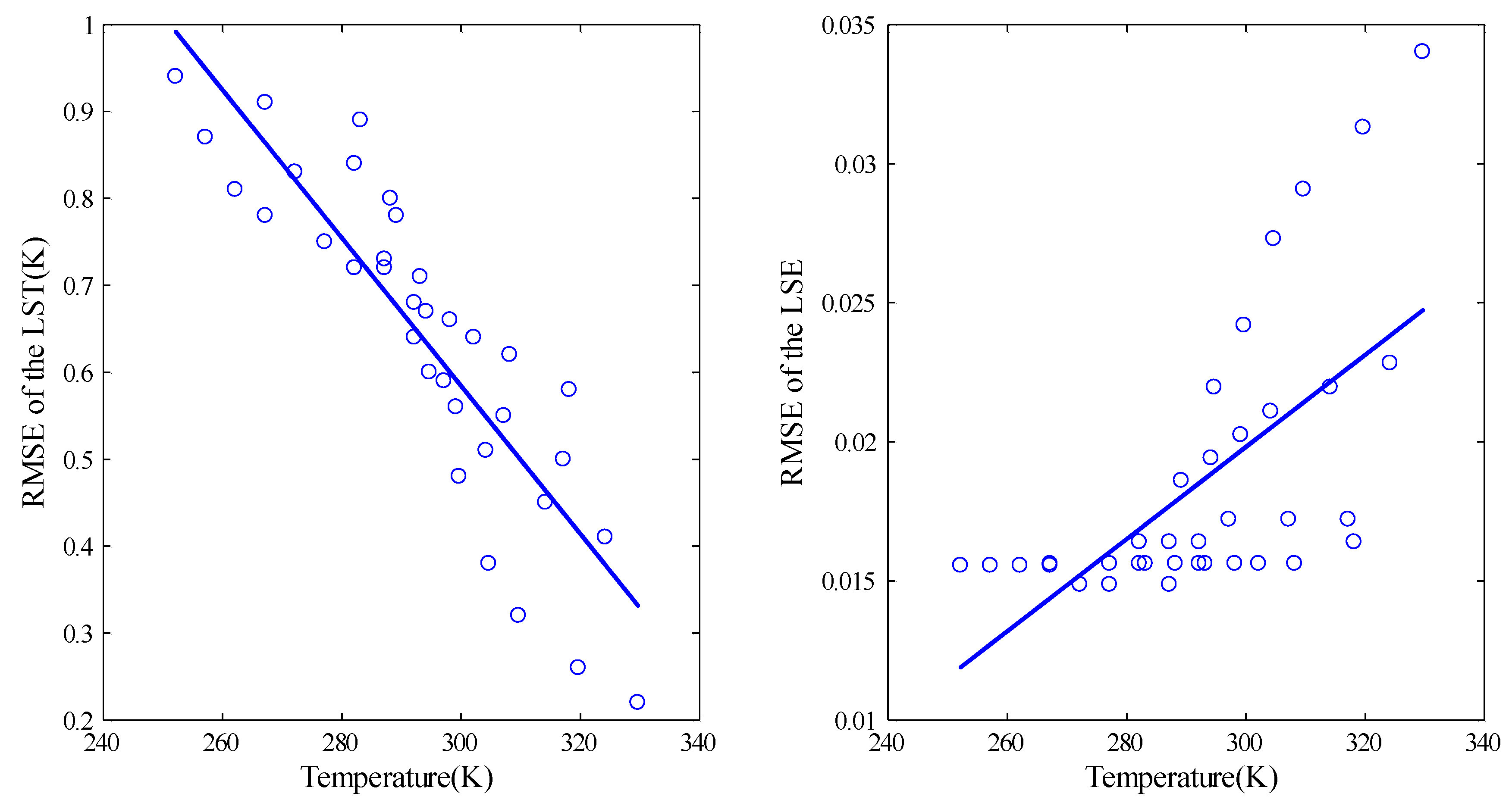
Therefore, through the ELD method, we can theoretically maintain the emissivity spectrum shape of the Landsat-8 TIRS data. To analyze the accuracy of the ELD method, simulation data of six model atmospheres from MODTRAN5 are utilized. By assuming one emissivity of the two TIRS bands is known, the emissivity of the other band is calculated using the ELD method. Then, the accuracy is evaluated and the results are shown in Figure 3. The RMSE of the calculated emissivity of band 10 and band 11 are 0.080 and 0.075, respectively, which demonstrate that the ELD method can be applied to maintain the emissivity spectral shape of TIRS data.

Figure 3. Accuracy evaluation of the ELD method based on the simulated dataset. The results are based on the simulation dataset by the MODTRAN model. (a) shows the comparison between the calculated and the reference emissivity of band 10, and (b) has a similar meaning. N is the number of simulation data, Bias is the average difference between the calculated and the reference emissivity, RMSE is the root mean square error.

Figure 3. Accuracy evaluation of the ELD method based on the simulated dataset. The results are based on the simulation dataset by the MODTRAN model. (a) shows the comparison between the calculated and the reference emissivity of band 10, and (b) has a similar meaning. N is the number of simulation data, Bias is the average difference between the calculated and the reference emissivity, RMSE is the root mean square error.

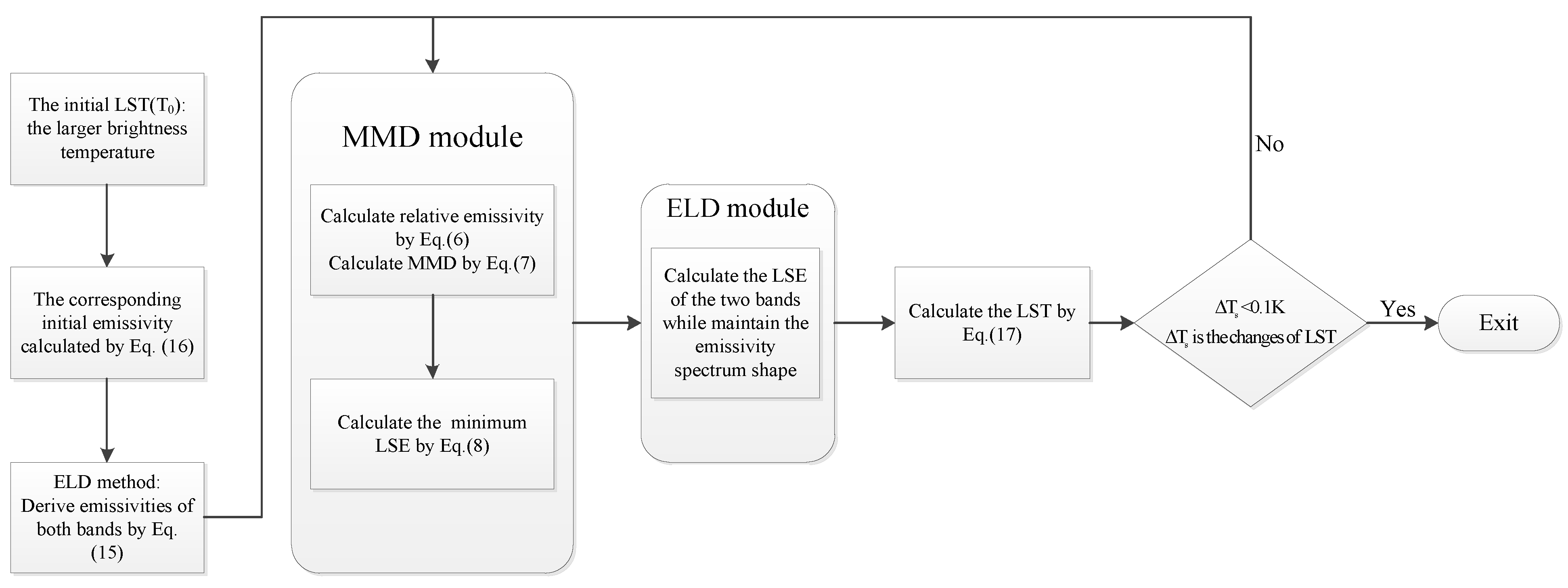
3.3. Procedures of the Algorithm

As discussed in Section 1, the TES algorithms are designed for and perform well with multispectral thermal data. The TES algorithms comprise of MMD method and ratio algorithm. Since simultaneously retrieving the LST and the LSE is a typical ill-posed problem, the MMD method is used to turn it into a well posed problem. The ratio algorithm is used to keep the shape of the emissivity spectrum, while it cannot be applied to Landsat-8 data. Similarly, the proposed TES algorithm for Landsat-8 data comprise of TIRS MMD module and ELD module. Based on the MMD module in Section 3.1, the ill-posed problem for separating the emissivity and temperature can be resolved. In order to maintain the emissivity spectrum shape, the ELD method is proposed based on the modified Wien’s approximation. Accuracy evaluation of the ELD method demonstrates that it can theoretically maintain the emissivity spectrum shape of the Landsat-8 TIRS data.

The procedures of the temperature and emissivity separation algorithm have been summarized as the following. Inputs to the algorithm include the atmospheric transmittance, atmospheric upwelling and downwelling radiances, the radiance at the TOA and the brightness temperature. The iterative process works as follows. Firstly, an initial LST ($T_0$) is set to be the larger brightness temperature between TIRS bands 10 and 11. The corresponding initial emissivity ${\text{ε}}_j$ is calculated by the following equation:

$${\text{ε}}_j=\frac{L_j^{ground}-L_{atj\downarrow }}{B_j\left(T_0\right)-L_{atj\downarrow }}$$

(16)

where j is the band whose brightness temperature is larger, and the initial emissivity of the other band is derived through the ELD method (namely Equation (15)). Secondly, the relative emissivity and the MMD are acquired, and the minimum emissivity can be estimated from the empirical relationship between MMD and ${\text{ε}}_{min}$ afterwards. The ELD method is utilized again to calculate the LSE of the two bands from ${\text{ε}}_{min}$, which could maintain the emissivity spectrum shape. After that, because the uncorrected out-of-field stray light of TIRS has a larger effect on band 11 [57], the LST is retrieved from the radiation transfer equation at band 10:

$$T_s=\frac{C_2}{{\lambda }_{10}}{\left(\ln \left(\frac{{\text{ε}}_{10}\cdot C_1}{\pi \cdot {{\lambda }_{10}}^5\cdot \left(L_{10}^{ground}-\left(1-{\text{ε}}_{10}\right)\cdot L_{at10\downarrow }\right)}+1\right)\right)}^{-1}$$

(17)

Figure 4. The flow chart of the algorithm in this study.

Figure 4. The flow chart of the algorithm in this study.

Using the calculated emissivities as the input values of the MMD module and the ELD module, this process is repeated until the change of the LST is less than 0.1 K. The change of the LST means the difference between the calculated LST of this iteration loop and the previous one. The flow chart of the algorithm is illustrated in Figure 4.

4. Results and Discussion

4.1. Algorithm Testing from the Simulated Data

The objective of this testing is to determine if the algorithm can accurately retrieve the surface emissivities and the LST values. The temperature and emissivity separation algorithm has been applied to the simulated data based on the model atmosphere of MODTRAN over the 96 emissivity spectra. Detailed parameter settings of the simulation are listed in Section 2.1. The results are shown in Table 3.

For the retrieved LST from the simulated data, the bias varies from 0.16 to 0.33 K, with an average of 0.21 K; the mean absolute error varies from 0.32 to 0.54 K, with an average of 0.48 K; the RMSE varies from 0.40 to 0.81 K, with an average of 0.67 K; and the correlation coefficient is 1.0. The histogram of the differences between the retrieved LST and the reference LST is shown in Figure 5. More than 62% of the retrieved results that differed from the actual LST are within 0.5 K, 94.3% are within 1.0 K and 97.9% are within 1.5 K. Although the algorithm gives a slight overestimation of the LST of about 0.2 K, it can retrieve the land surface temperature precisely. The RMSE of retrieval results is only 0.7 K, which is better than the single-channel algorithm (about 1.7 K) and the split-window algorithm (about 1 K) [34,58].

Figure 5. Histogram of the differences between the retrieved LST and the reference LST.

Figure 5. Histogram of the differences between the retrieved LST and the reference LST.

Table 3. Test results of the algorithm from the simulated data. Bias (the LST/LSE retrieved from the algorithm minus the reference LST/LSE), Mean absolute errors (Mean), RMSE values of the LST/LSE and linear correlation coefficient (R) are shown.

Model Atmosphere	Temperature (K)				Emissivity(10 band)				Emissivity(11 band)
	Bias	Mean	RMSE	R	Bias	Mean	RMSE	R	Bias	Mean	RMSE	R
Tropical	0.19	0.32	0.40	1.0	0.008	0.016	0.025	0.96	0.003	0.009	0.013	0.86
Mid-Latitude Summer	0.33	0.48	0.58	1.0	−0.002	0.014	0.017	0.98	0.000	0.008	0.011	0.87
Mid-Latitude Winter	0.16	0.51	0.76	1.0	−0.004	0.008	0.012	0.97	−0.001	0.007	0.010	0.84
Mid-Arctic Summer	0.30	0.51	0.65	1.0	−0.004	0.011	0.014	0.98	−0.001	0.007	0.010	0.86
Mid-Arctic Winter	0.03	0.51	0.81	1.0	−0.002	0.008	0.011	0.97	−0.000	0.007	0.011	0.83
1976 U.S. Standard	0.28	0.54	0.71	1.0	−0.005	0.010	0.012	0.98	−0.002	0.007	0.010	0.85
All	0.21	0.48	0.67	1.0	−0.002	0.011	0.016	0.95	0.000	0.007	0.011	0.83

Table 3. Test results of the algorithm from the simulated data. Bias (the LST/LSE retrieved from the algorithm minus the reference LST/LSE), Mean absolute errors (Mean), RMSE values of the LST/LSE and linear correlation coefficient (R) are shown.

Model Atmosphere	Temperature (K)				Emissivity(10 band)				Emissivity(11 band)
	Bias	Mean	RMSE	R	Bias	Mean	RMSE	R	Bias	Mean	RMSE	R
Tropical	0.19	0.32	0.40	1.0	0.008	0.016	0.025	0.96	0.003	0.009	0.013	0.86
Mid-Latitude Summer	0.33	0.48	0.58	1.0	−0.002	0.014	0.017	0.98	0.000	0.008	0.011	0.87
Mid-Latitude Winter	0.16	0.51	0.76	1.0	−0.004	0.008	0.012	0.97	−0.001	0.007	0.010	0.84
Mid-Arctic Summer	0.30	0.51	0.65	1.0	−0.004	0.011	0.014	0.98	−0.001	0.007	0.010	0.86
Mid-Arctic Winter	0.03	0.51	0.81	1.0	−0.002	0.008	0.011	0.97	−0.000	0.007	0.011	0.83
1976 U.S. Standard	0.28	0.54	0.71	1.0	−0.005	0.010	0.012	0.98	−0.002	0.007	0.010	0.85
All	0.21	0.48	0.67	1.0	−0.002	0.011	0.016	0.95	0.000	0.007	0.011	0.83

The algorithm not only can retrieve the LST with high accuracy, but it also can estimate the surface emissivities on the basis of accurate atmospheric correction. As shown in Table 3, both the emissivities of TIRS band 10 and 11 can be derived with almost no bias. Moreover, their mean absolute errors are about 0.011 and 0.007, respectively. Although the correlation coefficient is only 0.83, the RMSE of emissivity in band 11 is only 0.011, which is actually more accurate than band 10 with a RMSE of 0.016. The histogram of the differences between the retrieved LSE and the reference LSE are shown in Figure 6. More than 53.2% of the retrieved results that differed from the actual LSE are within 0.010, 82.1% are within 0.015 for band 10; and more than 80.9% are within 0.010, 92.3% are within 0.015 for band 11. As shown in the left part of Figure 6, the retrieved surface emissivities of TIRS band 10 have a slight underestimation, unlike band 11. However, the retrieved LSE may be higher than the actual LSE in some cases, which can be seen in Figure 6. The uncertainty of the empirical equation in the MMD module and the error of the atmospheric correction in the ELD module could be the reasons.

Figure 6. Histogram of the differences between the retrieved LSE and the reference LSE.

Figure 6. Histogram of the differences between the retrieved LSE and the reference LSE.

As shown in Table 3, the RMSE of temperature increases when moisture decreases from tropical to polar, while the RMSE of emissivities are opposite. Under normal circumstances, more moisture results in worse retrieval. Additionally, the scene temperature is also an important factor that affects the retrievals of the LST. Because the temperature decreases from tropical to polar, so does the brightness temperature. Cold scenes have larger observation noises in brightness temperature, which will result in worse retrievals. In order to analyze the influence of the brightness temperature, the RMSE of LST and LSE are calculated according to different temperatures, which are presented in Figure 7. Results show that the RMSE of LST increases when the temperature decreases from tropical to polar, while the RMSE of LSE decreases. Therefore, compared to the moisture, observation noises have larger effects on the LST retrievals.

Figure 7. The RMSE of LST and LSE according to different temperatures.

Figure 7. The RMSE of LST and LSE according to different temperatures.

To further analyze the accuracy and the practicability of the algorithm for different surface types, we summarize the performance corresponding to different laboratory spectra types. The results are shown in Table 4. As shown in Table 4, the algorithm developed in this paper can provide the best results of LST for surfaces with soil and stones, and their RMSE are about 0.42 K and 0.49 K, respectively. Moreover, the accuracy of the retrieved surface emissivity is about 0.010 (RMSE value), which is much better than vegetated surfaces. However, the retrieved surface emissivities have a slight bias for both soils and stones. For surfaces with water, snow and ice, the algorithm can provide moderate accuracy for both the LST and the LSE. Nevertheless, the accuracy of the algorithm is the worst for the vegetated surfaces, whose RMSE of the LST is greater than 2 K and the RMSE of the LSEs are greater than 0.035. It is possibly because the emissivity spectra from vegetation types do not fit the MMD module perfectly (Equation (8)), which can be seen from Figure 2. Besides, the temperature and emissivity separation algorithms will provide a worse result for low spectral contrast surfaces, such as high-vegetated areas, which have been demonstrated by the ASTER TES algorithm [19]. Some studies have been conducted to solve the problems [42], thus further efforts are needed to analyze the algorithm for vegetation surfaces in the future.

Table 4. Accuracy of the algorithm for different surface types.

Surface Type	Number of Cases	Temperature (K)			Emissivity(10 Band)			Emissivity(11 Band)
		Bias	Mean	RMSE	Bias	Mean	RMSE	Bias	Mean	RMSE
Vegetation	144	−0.76	1.80	2.16	0.012	0.032	0.035	0.016	0.032	0.037
Water/Snow/Ice	216	0.70	0.70	0.79	−0.014	0.014	0.015	−0.005	0.008	0.009
Soil	1872	0.38	0.43	0.49	−0.008	0.009	0.010	−0.004	0.005	0.006
Stone	1188	0.00	0.34	0.42	0.008	0.012	0.016	0.004	0.007	0.009

Table 4. Accuracy of the algorithm for different surface types.

Surface Type	Number of Cases	Temperature (K)			Emissivity(10 Band)			Emissivity(11 Band)
		Bias	Mean	RMSE	Bias	Mean	RMSE	Bias	Mean	RMSE
Vegetation	144	−0.76	1.80	2.16	0.012	0.032	0.035	0.016	0.032	0.037
Water/Snow/Ice	216	0.70	0.70	0.79	−0.014	0.014	0.015	−0.005	0.008	0.009
Soil	1872	0.38	0.43	0.49	−0.008	0.009	0.010	−0.004	0.005	0.006
Stone	1188	0.00	0.34	0.42	0.008	0.012	0.016	0.004	0.007	0.009

The atmospheric profiles used in the algorithm are one of the biggest sources of errors in LST and LSE retrievals. A sensitivity analysis has been performed to assess the uncertainty of the LST in response to errors in the atmospheric profiles. The six model atmospheres in MODTRAN are used. The effect of atmospheric profile uncertainties is simulated in two ways [50]. First, the air temperature varies by 1 K at each level. Second, the water vapor content is changed by 10% at each profile level. The difference (in absolute value) between the LST calculated with the modified and the original profile is the corresponding LST error. The total uncertainty is the RMSE of the above. Detailed results are shown in Table 5. According to these results, water vapor content is the larger source of errors in the LST retrievals, while air temperature has a lower impact. Because moisture decreases from tropical to polar, so does the imposed uncertainty of water vapor. Thus, the impact of the water vapor on the LST retrieval decreases from tropical to polar. Overall, the uncertainties of LST in response to air temperature error and water vapor error are 0.60 K and 0.98 K, respectively.

Table 5. Uncertainty of the derived LST/LSE for different sources of uncertainty.

Model Atmosphere	Air Temperature (1K)			Water Vapor (10%)
	LSE (Band 10)	LSE (Band 11)	LST (K)	LSE (Band 10)	LSE (Band 11)	LST (K)
Tropical	0.008	0.003	1.05	0.016	0.007	1.63
Mid-Latitude Summer	0.012	0.009	0.70	0.013	0.006	1.22
Mid-Latitude Winter	0.003	0.001	0.32	0.005	0.003	0.42
Mid-Arctic Summer	0.004	0.002	0.56	0.011	0.005	1.02
Mid-Arctic Winter	0.002	0.001	0.20	0.003	0.002	0.24
1976 U.S. Standard	0.003	0.001	0.34	0.007	0.003	0.56
All	0.006	0.004	0.60	0.010	0.005	0.98

Table 5. Uncertainty of the derived LST/LSE for different sources of uncertainty.

Model Atmosphere	Air Temperature (1K)			Water Vapor (10%)
	LSE (Band 10)	LSE (Band 11)	LST (K)	LSE (Band 10)	LSE (Band 11)	LST (K)
Tropical	0.008	0.003	1.05	0.016	0.007	1.63
Mid-Latitude Summer	0.012	0.009	0.70	0.013	0.006	1.22
Mid-Latitude Winter	0.003	0.001	0.32	0.005	0.003	0.42
Mid-Arctic Summer	0.004	0.002	0.56	0.011	0.005	1.02
Mid-Arctic Winter	0.002	0.001	0.20	0.003	0.002	0.24
1976 U.S. Standard	0.003	0.001	0.34	0.007	0.003	0.56
All	0.006	0.004	0.60	0.010	0.005	0.98

4.2. Algorithm Validation Based on SURFRAD Ground Measurements

Since the datasets have hardly any error, algorithm validation by simulated data can only reveal the accuracy of the method itself. However, in addition to the inner precision of the algorithm, the accuracy of the temperature and emissivity algorithms depends largely on the errors of the calibration, atmospheric correction and radiometric noises. To further evaluate the algorithm, comparisons have been conducted between the retrieval results from the real Landsat-8 TIRS data and the referenced LST based on SURFRAD ground measurements. Four SURFRAD sites are chosen in this study. The atmospheric profiles and software used in this study and the processing of the Landsat-8 images are listed in Section 2. The validation results are shown in Table 6.

Figure 8 shows the scatterplots of the comparison between the LST from Landsat-8 TIRS data and the LST from ground-based measurements at four SURFRAD sites. Table 7 summarizes the statistical parameters of the comparison by each SURFRAD ground site. Figure 8 demonstrates that the two LSTs agree well for most cases at the four sites, whose correlation coefficients are about 0.99 for all sites. The bias in three sites varies from −0.70 to 0.74 K and one site has a 1.69 K bias, with an average of 0.66 K. Maybe the number of cases is too few to include all the circumstances, and the LSTs calculated from SURFRAD ground measurements have about a −0.3 K bias during daytime. The average mean absolute error over the four sites is 1.74 K and varies from 1.04 to 2.56 K. The RMSE varies from 1.42 to 3.34 K, with an average of 2.32 K. Of all the 40 cases, 45% of the retrieved LSTs that differed from the actual LST are within 1 K, and 62.5% are within 2 K.

Table 6. Validation cases based on the SURFRAD ground measurements. Retrieved LST/LSE means the LST/LSE is retrieved from satellite images by the algorithm in this study, the reference LST means the LST is calculated from SURFRAD ground measurements. Bias is the retrieved LST minus the reference LST.

Sites	Time (d/m/y)	Retrieved LST (K)	Reference LST (K)	Bias (K)	Retrieved LSE
					10 Band	11 Band
Bondville	22 April 2013	297.56	295.07	2.48	0.944	0.965
	28 August 2013	307.58	306.78	0.80	0.967	0.974
	18 December 2013	261.98	265.10	−3.12	0.970	0.957
	11 February 2014	258.73	259.37	−0.64	0.944	0.964
	16 April 2014	287.13	286.48	0.65	0.969	0.953
	18 May 2014	300.03	295.93	4.10	0.980	0.978
	3 June 2014	304.33	302.41	1.92	0.979	0.977
	23 September 2014	296.00	296.20	−0.19	0.982	0.982
	25 October 2014	294.31	293.65	0.65	0.981	0.979
Goodwin Creek	11 July 2013	287.61	286.05	1.56	0.973	0.963
	25 December 2013	280.18	280.89	−0.70	0.969	0.953
	27 February 2014	284.61	285.96	−1.35	0.974	0.965
	16 April 2014	294.07	294.83	−0.75	0.976	0.970
	5 July 2014	303.35	305.50	−2.15	0.979	0.977
	6 August 2014	306.86	307.24	−0.37	0.977	0.972
	22 August 2014	307.17	307.23	−0.06	0.964	0.973
	23 September 2014	302.25	302.76	−0.51	0.947	0.966
	10 November 2014	293.10	295.02	−1.92	0.969	0.954
Sioux Falls	10 June 2013	305.65	301.00	4.65	0.968	0.975
	12 July 2013	308.30	305.04	3.26	0.976	0.970
	28 July 2013	305.39	300.01	5.38	0.970	0.956
	29 August 2013	310.09	307.75	2.34	0.973	0.964
	16 October 2013	287.50	286.75	0.75	0.971	0.959
	1 November 2014	285.52	285.28	0.24	0.967	0.948
	25 March 2014	277.37	276.26	1.10	0.970	0.956
	28 May 2014	306.76	305.45	1.32	0.971	0.976
	29 June 2014	307.26	304.98	2.28	0.965	0.944
	17 September 2014	299.11	298.97	0.13	0.979	0.977
	19 October 2014	294.38	295.09	−0.70	0.975	0.978
	4 November 2014	284.64	285.13	−0.49	0.973	0.965
Fort Peck	6 July 2013	304.40	301.23	3.17	0.981	0.980
	24 September 2013	300.31	297.96	2.35	0.962	0.973
	26 October 2013	284.11	284.87	−0.76	0.971	0.959
	11 November 2013	270.42	270.49	−0.07	0.963	0.938
	19 March 2014	278.92	284.60	−5.69	0.969	0.955
	9 July 2014	314.79	309.81	4.97	0.976	0.970
	25 July 2014	306.20	303.37	2.84	0.964	0.973
	26 August 2014	300.03	298.99	1.04	0.983	0.982
	13 October 2014	295.12	295.03	0.09	0.981	0.982
	30 November 2014	252.58	254.77	−2.20	0.947	0.973

Table 6. Validation cases based on the SURFRAD ground measurements. Retrieved LST/LSE means the LST/LSE is retrieved from satellite images by the algorithm in this study, the reference LST means the LST is calculated from SURFRAD ground measurements. Bias is the retrieved LST minus the reference LST.

Sites	Time (d/m/y)	Retrieved LST (K)	Reference LST (K)	Bias (K)	Retrieved LSE
					10 Band	11 Band
Bondville	22 April 2013	297.56	295.07	2.48	0.944	0.965
	28 August 2013	307.58	306.78	0.80	0.967	0.974
	18 December 2013	261.98	265.10	−3.12	0.970	0.957
	11 February 2014	258.73	259.37	−0.64	0.944	0.964
	16 April 2014	287.13	286.48	0.65	0.969	0.953
	18 May 2014	300.03	295.93	4.10	0.980	0.978
	3 June 2014	304.33	302.41	1.92	0.979	0.977
	23 September 2014	296.00	296.20	−0.19	0.982	0.982
	25 October 2014	294.31	293.65	0.65	0.981	0.979
Goodwin Creek	11 July 2013	287.61	286.05	1.56	0.973	0.963
	25 December 2013	280.18	280.89	−0.70	0.969	0.953
	27 February 2014	284.61	285.96	−1.35	0.974	0.965
	16 April 2014	294.07	294.83	−0.75	0.976	0.970
	5 July 2014	303.35	305.50	−2.15	0.979	0.977
	6 August 2014	306.86	307.24	−0.37	0.977	0.972
	22 August 2014	307.17	307.23	−0.06	0.964	0.973
	23 September 2014	302.25	302.76	−0.51	0.947	0.966
	10 November 2014	293.10	295.02	−1.92	0.969	0.954
Sioux Falls	10 June 2013	305.65	301.00	4.65	0.968	0.975
	12 July 2013	308.30	305.04	3.26	0.976	0.970
	28 July 2013	305.39	300.01	5.38	0.970	0.956
	29 August 2013	310.09	307.75	2.34	0.973	0.964
	16 October 2013	287.50	286.75	0.75	0.971	0.959
	1 November 2014	285.52	285.28	0.24	0.967	0.948
	25 March 2014	277.37	276.26	1.10	0.970	0.956
	28 May 2014	306.76	305.45	1.32	0.971	0.976
	29 June 2014	307.26	304.98	2.28	0.965	0.944
	17 September 2014	299.11	298.97	0.13	0.979	0.977
	19 October 2014	294.38	295.09	−0.70	0.975	0.978
	4 November 2014	284.64	285.13	−0.49	0.973	0.965
Fort Peck	6 July 2013	304.40	301.23	3.17	0.981	0.980
	24 September 2013	300.31	297.96	2.35	0.962	0.973
	26 October 2013	284.11	284.87	−0.76	0.971	0.959
	11 November 2013	270.42	270.49	−0.07	0.963	0.938
	19 March 2014	278.92	284.60	−5.69	0.969	0.955
	9 July 2014	314.79	309.81	4.97	0.976	0.970
	25 July 2014	306.20	303.37	2.84	0.964	0.973
	26 August 2014	300.03	298.99	1.04	0.983	0.982
	13 October 2014	295.12	295.03	0.09	0.981	0.982
	30 November 2014	252.58	254.77	−2.20	0.947	0.973

Figure 8. The comparison scatterplots of LST from Landsat-8 TIRS data and the LST from ground-based measurements at four SURFRAD sites. Data used here are from 2013 to 2014.

Figure 8. The comparison scatterplots of LST from Landsat-8 TIRS data and the LST from ground-based measurements at four SURFRAD sites. Data used here are from 2013 to 2014.

Table 7. Summaries of the validation results according to different ground sites. Bias, Mean, RMSE and R have the same meaning as Table 3.

Sites	Number of Cases	Temperature (K)
		Bias	Mean	RMSE	R
Bondville	9	0.74	1.62	2.34	0.996
Goodwin Creek	9	−0.70	1.04	1.42	0.994
Sioux Falls	12	1.69	1.89	2.52	0.989
Fort Peck	10	0.39	2.56	3.34	0.993
All	40	0.66	1.74	2.32	0.991

Table 7. Summaries of the validation results according to different ground sites. Bias, Mean, RMSE and R have the same meaning as Table 3.

Sites	Number of Cases	Temperature (K)
		Bias	Mean	RMSE	R
Bondville	9	0.74	1.62	2.34	0.996
Goodwin Creek	9	−0.70	1.04	1.42	0.994
Sioux Falls	12	1.69	1.89	2.52	0.989
Fort Peck	10	0.39	2.56	3.34	0.993
All	40	0.66	1.74	2.32	0.991

The errors may come from different sources. The majority of the error stems from the empirical equation between the minimum emissivity and the MMD, which is not a perfect fit for all cases. Three of the four sites are covered by vegetated surfaces, whose residuals in the MMD equation are especially high, thus resulting in bigger errors. The accuracy of calibration in TIRS channels also has a significant effect on the accuracy of the algorithm. Although a calibration update was implemented on 3 February 2014 in the USGS/EROS processing system for both bands to correct a bias error (0.29 and 0.51 W/m²·sr·μm or −2.1 K and −4.4 K at 300 K in Band 10 and 11, respectively), the residuals are still larger than desired for both bands (0.12 and 0.2 W/m²·sr·μm or 0.87 K and 1.67 K at 300 K). While the out-of-field stray light is small enough in band 10, the effect in band 11 is larger and studies suggest that band 11 data should not be used for quantitative analysis at present [57,59]. Therefore, the accuracy could be better if the calibration issue of TIRS band 11 is resolved in the future. Besides, the accuracy of the NCEP reanalysis datasets also will affect the accuracy of the algorithm. In summary, the algorithm can retrieve the LST with an average absolute error of 1.7 K, which is slightly worse than the split-window algorithm. However, since the temperature and emissivity algorithm does not need the LSE a priori, it can be used as an alternative method to retrieve the LST over the areas where the LSE is not known.

5. Conclusions

In this study, a temperature and emissivity separation algorithm is developed to simultaneously retrieve the LST and the LSE from Landsat-8 TIRS data. According to the radiative transfer equation, simultaneously retrieving the LST and the LSE from Landsat-8 TIRS is a typical ill-posed problem. However, by making full use of the information between the emissivities in different bands, the ill-posed problem can be resolved. Therefore, based on the laboratory emissivity spectra data, the MMD module for TIRS data is developed. Moreover, in order to maintain the emissivity spectrum shape in the iterative process, an emissivity log difference method (ELD method) is developed in this study, which is based on the modified Wien’s approximation. In support of the above studies, the LST and LSE can be recovered simultaneously from TIRS data.

The performance of the algorithm is examined based on the MODTRAN5 model and 96 emissivity spectra over natural surfaces. The RMSEs are 0.67 K, 0.016 and 0.011 for LST and the emissivities of bands 10 and 11, respectively. More than 94% of the retrieved results that differed from the actual LST are within 1.0 K. Results show that both the LST and LSE can be estimated with a good accuracy by the algorithm. In addition, this algorithm is practicable for different surface types including vegetation, water, snow, ice, soils and rocks. To further analyze the algorithm, the evaluation between the retrieved LST and the reference LST from SURFRAD ground measurements is conducted. The average absolute error of the LST is 1.7 K with an average bias of 0.6 K, which is better than the single-channel methods but slightly worse than the split-window algorithm [34]. The imperfect fit of the empirical equation in the MMD module and the calibration errors in the TIRS channels are the main sources which affect the accuracy of the algorithm. Therefore, the algorithm in this study makes it possible to retrieve the LST from Landsat-8 TIRS data without the prior knowledge of surface emissivity. Although there are some issues that need to be addressed in the future, such as the calibration errors of band 11, the algorithm consisting of the MMD and ELD modules is capable of retrieving the LST and LSE simultaneously from Landsat-8 TIRS data with good results.

References

1. Beeri, O.; Peled, A. Geographical model for precise agriculture monitoring with real-time remote sensing. ISPRS J. Photogramm. Remote Sens. 2009, 64, 47–54. [Google Scholar]
2. Hansen, J.; Ruedy, R.; Sato, M.; Lo, K. Global surface temperature change. Rev. Geophys. 2010, 48, RG4004. [Google Scholar]
3. Weng, Q. Thermal infrared remote sensing for urban climate and environmental studies: Methods, applications, and trends. ISPRS J. Photogramm. Remote Sens. 2009, 64, 335–344. [Google Scholar]
4. Xiong, Y.; Qiu, G. Estimation of evapotranspiration using remotely sensed land surface temperature and the revised three-temperature model. Int. J. Remote Sens. 2011, 32, 5853–5874. [Google Scholar]
5. Kalma, J.; McVicar, T.; McCabe, M. Estimating land surface evaporation: A review of methods using remotely sensed surface temperature data. Sury. Geophys. 2008, 29, 421–469. [Google Scholar]
6. Galleguillos, M.; Jacob, F.; Prévot, L.; French, A.; Lagacherie, P. Comparison of two temperature differencing methods to estimate daily evapotranspiration over a Mediterranean vineyard watershed from ASTER data. Remote Sens. Environ. 2011, 115, 1326–1340. [Google Scholar]
7. Anderson, M.; Kustas, W.; Norman, J. Upscaling flux observations from local to continental scales using thermal remote sensing. Agron. J. 2007, 99, 240–254. [Google Scholar]
8. Voogt, J.; Oke, T. Thermal remote sensing of urban climates. Remote Sens. Environ. 2003, 86, 370–384. [Google Scholar]
9. Berni, J.; Zarco-Tejada, P.; Suárez, L.; Fereres, E. Thermal and narrowband multispectral remote sensing for vegetation monitoring from an unmanned aerial vehicle. IEEE Trans. Geosci. Remote Sens. 2009, 47, 722–738. [Google Scholar]
10. Anderson, M.; Norman, J.; Kustas, W.; Houborg, R.; Starks, P.; Agam, N. A thermal-based remote sensing technique for routine mapping of land-surface carbon, water and energy fluxes from field to regional scales. Remote Sens. Environ. 2008, 112, 4227–4241. [Google Scholar]
11. Sobrino, J.; Raissouni, N.; Li, Z. A comparative study of land surface emissivity retrieval from NOAA data. Remote Sens. Environ. 2001, 75, 256–266. [Google Scholar]
12. Sobrino, J.; Jiménez-Muñoz, J.; Verhoef, W. Canopy directional emissivity: Comparison between models. Remote Sens. Environ. 2005, 99, 304–314. [Google Scholar]
13. Li, Z.; Wu, H.; Wang, N.; Qiu, S.; Sobrino, J.; Wan, Z.; Tang, B.; Yan, G. Land surface emissivity retrieval from satellite data. Int. J. Remote Sens. 2013, 34, 3084–3127. [Google Scholar]
14. Schmugge, T.; French, A.; Ritchie, J.; Rango, A.; Pelgrum, H. Temperature and emissivity separation from multispectral thermal infrared observations. Remote Sens. Environ. 2002, 79, 189–198. [Google Scholar]
15. Becker, F.; Li, Z. Towards a local split window method over land surfaces. Int. J. Remote Sens. 1990, 11, 369–393. [Google Scholar] [CrossRef]
16. Jiménez-Muñoz, J.; Sobrino, J. A generalized single-channel method for retrieving land surface temperature from remote sensing data. J. Geophys. Res. 2003, 108, D22. [Google Scholar] [CrossRef]
17. Wan, Z.; Dozier, J. A generalized split-window algorithm for retrieving land-surface temperature from space. IEEE Trans. Geosci. Remote Sens. 1996, 34, 892–905. [Google Scholar]
18. Mao, K.; Qin, Z.; Shi, J.; Gong, P. A practical split-window algorithm for retrieving land surface temperature from MODIS data. Int. J. Remote Sens. 2005, 26, 3181–3204. [Google Scholar] [CrossRef]
19. Gillespie, A.; Rokugawa, S.; Matsunaga, T.; Cothern, J.; Hook, S.; Kahle, A. A temperature and emissivity separation algorithm for Advanced Spaceborne Thermal Emission and Reflection Radiometer (ASTER) images. IEEE Trans. Geosci. Remote Sens. 1998, 36, 1113–1126. [Google Scholar] [CrossRef]
20. Sòria, G.; Sobrino, J. ENVISAT/AATSR derived land surface temperature over a heterogeneous region. Remote Sens. Environ. 2007, 111, 409–422. [Google Scholar] [CrossRef]
21. Sobrino, J.; Jiménez-Muñoz, J.; Paolini, L. Land surface temperature retrieval from LANDSAT TM 5. Remote Sens. Environ. 2004, 90, 434–440. [Google Scholar] [CrossRef]
22. Sobrino, J.; Li, Z.; Stoll, M.; Becker, F. Improvements in the split-window technique for land surface temperature determination. IEEE Trans. Geosci. Remote Sens. 1994, 32, 243–253. [Google Scholar] [CrossRef]
23. Wang, N.; Li, Z.; Tang, B.; Zeng, F.; Li, C. Retrieval of atmospheric and land surface parameters from satellite-based thermal infrared hyperspectral data using a neural network technique. Int. J. Remote Sens. 2013, 34, 3485–3502. [Google Scholar] [CrossRef]
24. Peres, L.; Dacamara, C.; Trigo, I.; Freitas, S. Synergistic use of the two-temperature and split-window methods for land-surface temperature retrieval. Int. J. Remote Sens. 2010, 31, 4387–4409. [Google Scholar] [CrossRef]
25. Roy, D.; Wulder, M.; Loveland, T.; Woodcock, C.; Allen, R.; Anderson, M.; Zhu, Z. Landsat-8: Science and product vision for terrestrial global change research. Remote Sens. Environ. 2014, 145, 154–172. [Google Scholar] [CrossRef]
26. Irons, J.; Dwyer, J.; Barsi, J. The next Landsat satellite: The Landsat data continuity mission. Remote Sens. Environ. 2012, 122, 11–21. [Google Scholar] [CrossRef]
27. Ren, H.; Du, C.; Liu, R.; Qin, Q.; Meng, J.; Li, Z.L.; Yan, G. Evaluation of radiometric performance for the thermal infrared sensor onboard Landsat 8. Remote Sens. 2014, 6, 12776–12788. [Google Scholar] [CrossRef]
28. Montanaro, M.; Levy, R.; Markham, B. On-orbit radiometric performance of the Landsat 8 thermal infrared sensor. Remote Sens. 2014, 6, 11753–11769. [Google Scholar] [CrossRef]
29. Qin, Z.; Karnieli, A.; Berliner, P. A mono-window algorithm for retrieving land surface temperature from Landsat TM data and its application to the Israel-Egypt border region. Int. J. Remote Sens. 2001, 22, 3719–3746. [Google Scholar] [CrossRef]
30. Jiménez-Muñoz, J.; Cristóbal, J.; Sobrino, J.; Sòria, G.; Ninyerola, M.; Pons, X. Revision of the single-channel algorithm for land surface temperature retrieval from Landsat thermal-infrared data. IEEE Trans. Geosci. Remote Sens. 2009, 47, 339–349. [Google Scholar] [CrossRef]
31. Dash, P.; Göttsche, F.; Olesen, F.; Fischer, H. Land surface temperature and emissivity estimation from passive sensor data: Theory and practice-current trends. Int. J. Remote Sens. 2002, 23, 2563–2594. [Google Scholar] [CrossRef]
32. Sobrino, J.; Jiménez-Muñoz, J. Land surface temperature retrieval from thermal infrared data: An assessment in the context of the Surface Processes and Ecosystem Changes through Response Analysis (SPECTRA) mission. J. Geophys. Res. 2005, 110. [Google Scholar] [CrossRef]
33. Jiménez-Muñoz, J.; Sobrino, J. A single-channel algorithm for land-surface temperature retrieval from ASTER data. IEEE Trans. Geosci. Remote Sens. 2010, 7, 176–179. [Google Scholar] [CrossRef]
34. Jimenez-Munoz, J.; Sobrino, J.; Skokovic, D.; Mattar, C.; Cristóbal, J. Land surface temperature retrieval methods from Landsat-8 Thermal Infrared Sensor data. IEEE Trans. Geosci. Remote Sens. 2014, 11, 1840–1843. [Google Scholar] [CrossRef]
35. Du, C.; Ren, H.; Qin, Q.; Meng, J.; Zhao, S. A practical split-window algorithm for estimating land surface temperature from Landsat 8 data. Remote Sens. 2015, 7, 647–665. [Google Scholar] [CrossRef]
36. Rozenstein, O.; Qin, Z.; Derimian, Y.; Karnieli, A. Derivation of land surface temperature for Landsat-8 TIRS using a split window algorithm. Sensors 2014, 14, 5768–5780. [Google Scholar] [CrossRef] [PubMed]
37. Yang, L.; Cao, Y.; Zhu, X.; Zeng, S.; Yang, G.; He, J.; Yang, X. Land surface temperature retrieval for arid regions based on Landsat-8 TIRS data: A case study in Shihezi, Northwest China. J. Arid Land. 2014, 6, 704–716. [Google Scholar] [CrossRef]
38. Li, Z.; Becker, F. Properties and comparison of temperature-independent thermal infrared spectral indices with NDVI for HAPEX data. Remote Sens. Environ. 1990, 33, 165–182. [Google Scholar] [CrossRef]
39. Hook, S.; Gabell, A.; Green, A.; Kealy, P. A comparison of techniques for extracting emissivity information from thermal infrared data for geologic studies. Remote Sens. Environ. 1992, 42, 123–135. [Google Scholar] [CrossRef]
40. Wan, Z.; Li, Z. A physics-based algorithm for retrieving land-surface emissivity and temperature from EOS/MODIS data. IEEE Trans. Geosci. Remote Sens. 1997, 35, 980–996. [Google Scholar]
41. Kealy, P.; Hook, S. Separating temperature and emissivity in thermal infrared multispectral scanner data: Implications for recovering land surface temperatures. IEEE Trans. Geosci. Remote Sens. 1993, 31, 1155–1164. [Google Scholar] [CrossRef]
42. Coll, C.; Caselles, V.; Valor, E.; Niclòs, R.; Sánchez, J.; Galve, J.; Mira, M. Temperature and emissivity separation from ASTER data for low spectral contrast surfaces. Remote Sens. Environ. 2007, 110, 162–175. [Google Scholar] [CrossRef]
43. Hulley, G.; Hook, S. Generating consistent land surface temperature and emissivity products between ASTER and MODIS data for earth science research. IEEE Trans. Geosci. Remote Sens. 2011, 49, 1304–1315. [Google Scholar] [CrossRef]
44. Sobrino, J.; Jiménez-Muñoz, J.; Sòria, G.; Romaguera, M.; Guanter, L.; Moreno, J.; Plaza, A.; Martínez, P. Land surface emissivity retrieval from different VNIR and TIR sensors. IEEE Trans. Geosci. Remote Sens. 2008, 46, 316–327. [Google Scholar] [CrossRef]
45. Berk, A.; Anderson, G.; Acharya, P.; Bernstein, L.; Muratov, L.; Lee, J.; Lewis, P. MODTRAN 5: A reformulated atmospheric band model with auxiliary species and practical multiple scattering options: Update. Proc. SPIE 2005. [Google Scholar] [CrossRef]
46. Augustine, J.; DeLuisi, J.; Long, C. SURFRAD-A national surface radiation budget network for atmospheric research. Bull. Amer. Meteorol. Soc. 2000, 81, 2341–2357. [Google Scholar] [CrossRef]
47. Augustine, J.; Hodges, G.; Cornwall, C.; Michalsky, J.; Medina, C. An update on SURFRAD—The GCOS Surface Radiation budget network for the continental United States. J. Atmos. Ocean Technol. 2005, 22, 1460–1472. [Google Scholar] [CrossRef]
48. Wang, K.; Wan, Z.; Wang, P.; Sparrow, M.; Liu, J.; Zhou, X.; Haginoya, S. Estimation of surface long wave radiation and broadband emissivity using Moderate Resolution Imaging Spectroradiometer (MODIS) land surface temperature/emissivity products. J. Geophys. Res. 2005, 110. [Google Scholar] [CrossRef]
49. Wang, K.; Liang, S. Evaluation of ASTER and MODIS land surface temperature and emissivity products using long-term surface longwave radiation observations at SURFRAD sites. Remote Sens. Environ. 2009, 113, 1556–1565. [Google Scholar] [CrossRef]
50. Coll, C.; Caselles, V.; Valor, E.; Niclòs, R. Comparison between different sources of atmospheric profiles for land surface temperature retrieval from single channel thermal infrared data. Remote Sens. Environ. 2012, 117, 199–210. [Google Scholar] [CrossRef]
51. Kalnay, E.; Kanamitsu, M.; Kistler, R.; Collins, W.; Deaven, D.; Gandin, L.; Joseph, D. The NCEP/NCAR 40-year reanalysis project. Bull. Am. Meteor. Soc. 1996, 77, 437–471. [Google Scholar] [CrossRef]
52. Barsi, J.; Barker, J.; Schott, J. An atmospheric correction parameter calculator for a single thermal band earth-sensing instrument. In Proceedings of the IEEE International Geoscience and Remote Sensing Symposium (IGARSS), Toulouse, France, 21–25 July 2003; pp. 3014–3016.
53. Jiménez-Muñoz, J.; Sobrino, J.; Mattar, C.; Mattar, C.; Franch, B. Atmospheric correction of optical imagery from MODIS and Reanalysis atmospheric products. Remote Sens. Environ. 2010, 114, 2195–2210. [Google Scholar] [CrossRef]
54. Baldridge, A.; Hook, S.; Grove, C.; Rivera, G. The ASTER spectral library version 2.0. Remote Sens. Environ. 2009, 113, 711–715. [Google Scholar] [CrossRef]
55. Payan, V.; Royer, A. Analysis of Temperature Emissivity Separation (TES) algorithm applicability and sensitivity. Int. J. Remote Sens. 2004, 25, 15–37. [Google Scholar] [CrossRef]
56. Li, Z.; Becker, F. Feasibility of land surface temperature and emissivity determination from AVHRR data. Remote Sens. Environ. 1993, 43, 67–85. [Google Scholar] [CrossRef]
57. Barsi, J.; Schott, J.; Hook, S.; Raqueno, N.; Markham, B.; Radocinski, R. Landsat-8 Thermal Infrared Sensor (TIRS) vicarious radiometric calibration. Remote Sens. 2014, 6, 11607–11626. [Google Scholar] [CrossRef]
58. Yu, X.; Guo, X.; Wu, Z. Land surface temperature retrieval from Landsat 8 TIRS—Comparison between radiative transfer equation-based method, split window algorithm and single channel method. Remote Sens. 2014, 6, 9829–9852. [Google Scholar] [CrossRef]
59. Cook, M.; Schott, J.; Mandel, J.; Raqueno, N. Development of an operational calibration methodology for the Landsat thermal data archive and initial testing of the atmospheric compensation component of a Land Surface Temperature (LST) product from the archive. Remote Sens. 2014, 6, 11244–11266. [Google Scholar] [CrossRef]