An Improved Physics-Based Model for Topographic Correction of Landsat TM Images

Abstract

Optical remotely sensed images in mountainous areas are subject to radiometric distortions induced by topographic effects, which need to be corrected before quantitative applications. Based on Li model and Sandmeier model, this paper proposed an improved physics-based model for the topographic correction of Landsat Thematic Mapper (TM) images. The model employed Normalized Difference Vegetation Index (NDVI) thresholds to approximately divide land targets into eleven groups, due to NDVI’s lower sensitivity to topography and its significant role in indicating land cover type. Within each group of terrestrial targets, corresponding MODIS BRDF (Bidirectional Reflectance Distribution Function) products were used to account for land surface’s BRDF effect, and topographic effects are corrected without Lambertian assumption. The methodology was tested with two TM scenes of severely rugged mountain areas acquired under different sun elevation angles. Results demonstrated that reflectance of sun-averted slopes was evidently enhanced, and the overall quality of images was improved with topographic effect being effectively suppressed. Correlation coefficients between Near Infra-Red band reflectance and illumination condition reduced almost to zero, and coefficients of variance also showed some reduction. By comparison with the other two physics-based models (Sandmeier model and Li model), the proposed model showed favorable results on two tested Landsat scenes. With the almost half-century accumulation of Landsat data and the successive launch and operation of Landsat 8, the improved model in this paper can be potentially helpful for the topographic correction of Landsat and Landsat-like data.

1. Introduction

Mountain areas account for approximately 1/5 of the world’s land area, and provide diverse goods and services to human society [1]. Meanwhile, mountain ecosystems are the sensitive indicators to the rapid global development. It is essentially important to monitor the mountain ecosystem change and protect the mountain environment [2]. The development of remote sensing technique has unprecedentedly facilitated the detection of change and development in mountainous areas. Nevertheless, many difficulties and challenges are encountered in the remote sensing applications in mountainous areas. Compared to horizontal land surfaces, remotely sensed images of rugged areas possess pronounced topographic effect, which severely impacts the accuracy of the images’ quantitative applications [3]. Firstly, rugged terrain re-distributes the solar irradiance received by the terrestrial surfaces. Sun-facing slopes receive apparently more radiation than sun-averted slopes (except for shadowed sun-facing areas), and the recorded signals by satellite sensors from identical land cover type but different slope orientations may differ [4]. Secondly, tilted surfaces modify the angular configuration of sun-target-sensor (STS) geometry [5]. As for the ubiquitous non-Lambertian targets in the real world [6], different STS geometry often means different bi-directional reflectance (effect of bidirectional reflectance distribution function, BRDF) [7]. And this will very likely lead to phenomenon of the “same targets showing different reflectance and different targets showing same reflectance”, which severely reduces the accuracy of quantitative applications of remote sensing, such as biophysical parameter inversion and land use/cover change detection [8,9]. Therefore, topographic correction, aiming at elimination or at least reduction of terrain effect, is a necessity before the imagery of mountainous areas is used in quantitative analysis.

Previous contributions have reported a lot about empirical or semi-empirical topographic correction models, like cosine correction, C correction, SCS correction and SCS+C correction [10,11,12,13]. Cosine correction model treats the land surfaces as Lambertian and only adjusts the direct solar irradiance with simple cosine formula. This model tends to cause severe over-correction when local incidence angle is high [14,15]. C correction model reduces the over-correction to some extent by adding the C correction factor, obtained from the statistical relationship between the cosine of the relative solar incident angle and radiance received by the sensor [16,17]. Considering that trees are geotropic and topography has no control over the sun-crown geometry, Gu and Gillespie (1998) proposed the SCS correction model to correct topographic effects on forest images. However, over-correction still exists for faintly illuminated slopes in the SCS model [10]. Based on SCS and C correction models, Soenen et al. (2005) introduced a semi-empirical C factor to account for the diffuse irradiance and developed the SCS+C model [11]. Overall, the aforementioned models all assume that land surfaces are Lambertian, and only correct for the direct solar irradiance or compensate for the diffuse component using statistical method, which lacks sound physical bases.

Along with the further research on remote sensing theory and development of quantitative remote sensing, physics-based topographic correction models are developed based on the physical process between sunlight, atmosphere and land surface. The parameters in the physics-based model possess explicit mathematical and physical meanings. For example, Sandmeier and Itten (1997) employed the “Second Simulation of the Satellite Signal in the Solar Spectrum (6S)” model to calculate direct and diffuse solar irradiance, and then corrected them for terrain effect, respectively [5]. This model (referred to as Sandmeier model in the following) avoids the empirical regression in traditional methods, and possesses relatively solid physical foundation. However, with Lambertian assumption, it neglects the reflectance variance resulted from the BRDF effect [5]. Based on the Sandmeier method, Shepherd and Dymond (2003) not only compensated for the different components of illumination, but also normalized the image reflectance to horizontal surface and discussed the necessity of reflectance correction for images in rugged area [18]. Nevertheless, the reflectance of diffuse light is simplified and considered as isotropic, which does not seem reasonable, since diffuse sky light is directional, especially in sunny and misty days. Wen et al. (2009) developed a physics-based topographic correction model according to the fact that rugged terrain creates different configurations of STS geometry for the same land cover type, which can be used to derive BRDF shape function of that land cover type [19]. However, representative areas need to be selected and classification be conducted to obtain the reflective anisotropy information of each land cover type, which risks introducing relatively huge subjectivity. Considering the lack of multi-angular moderate-resolution data and depending on MODIS BRDF products (MCD43A1), Li et al. (2012) proposed a topographic correction model (referred to as Li model in the following) based on radiative transfer theory [20]. Topographic correction of Landsat Thematic Mapper (TM) images of Blue Mountain areas in Australia was conducted and satisfactory results were achieved. The methodology takes into account the BRDF effect and avoids the statistical analysis based on single scene, which helps maintain much more consistency and comparability for images acquired by different sensors or at different times. However, the experiment area selected by Li is only a small sub-scene, and the terrain ruggedness there is not so severe [20]. Moreover, digital surface model (DSM) used in correction is not readily available globally, and simply averaging MODIS parameters to characterize the BRDF effect of the whole study area may still need further discussion.

Landsat series satellites have operationally acquired land surface observation data for almost half a century. Along with the launch and successful in-orbit operation of Landsat 8, Landsat series imagery provides important data support for the research of China’s mountainous areas for the past 40 years and foreseeable future [21]. As discussed above, and in much literature [18,20], the BRDF effects and radiometric distortions by topographic effects in TM and TM-like fine spatial resolution images need to be considered in the applications in mountainous regions. Thus, studies on topographic correction accounting for BRDF effects are of great practical significance. In this study, we modified Li’s physics-based topographic correction model mainly by using NDVI-dependent MODIS BRDF parameters, and the specific objectives were to (1) compare the modified model’s performance with that of Sandmeier model (with Lambertian assumption) and Li model (without Lambertian assumption); and (2) attempt to improve the physics-based model to further facilitate and generalize the topographic correction of TM and TM-like imagery.

2. Study Area and Data

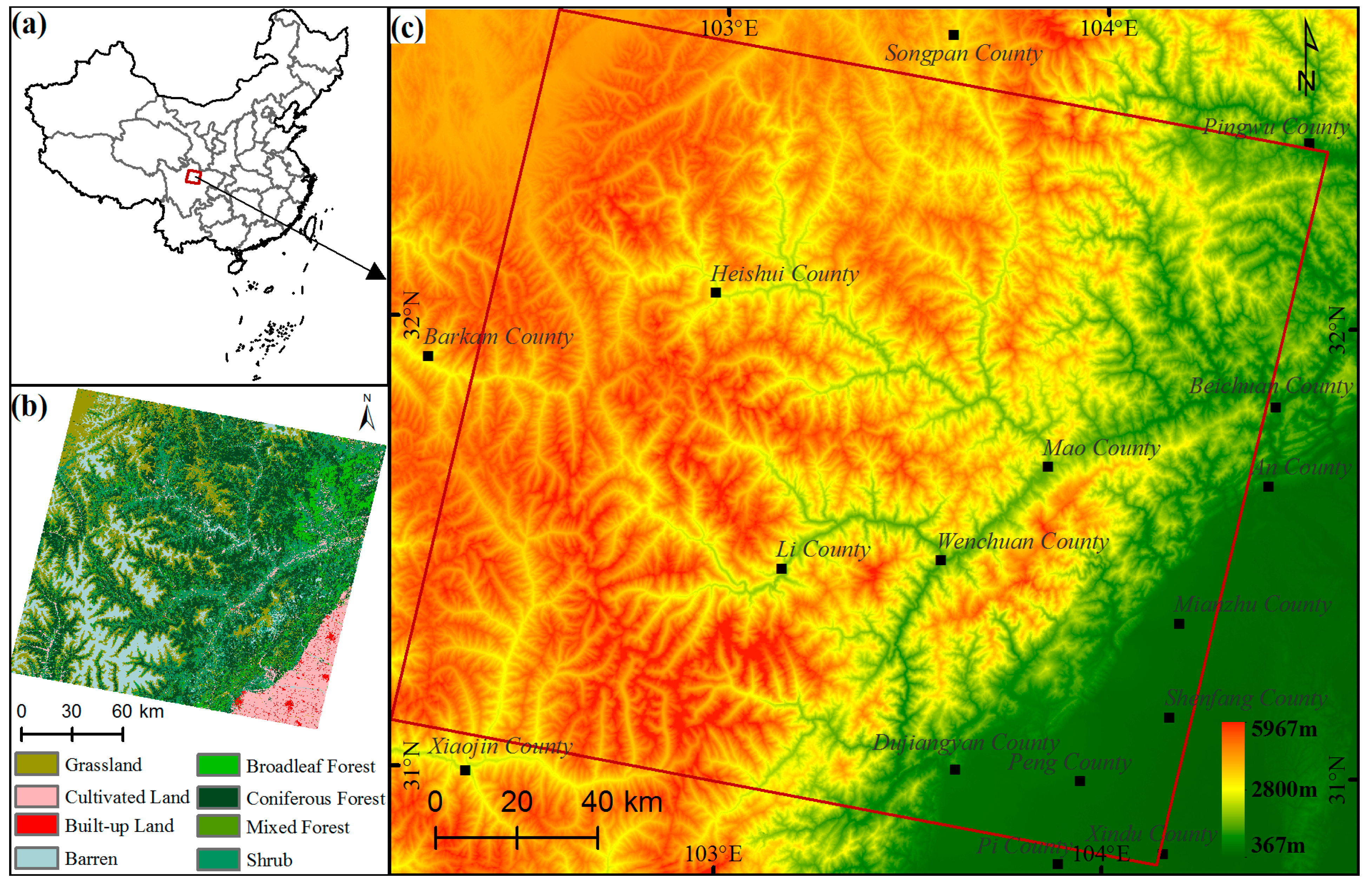
2.1. Study Area

The study area is located in the central part of the Hengduan Mountains, southeast to the Qinghai-Tibetan Plateau. It mainly covers Heishui County, Mao County, Li County and Wenchuan County of Sichuan Province, China (Figure 1). High mountain ranges and deep gullies dominate the landform of this area, and make the terrain undulation here tremendously severe. The altitude ranges from about 350 m to more than 5900 m, with an overall trend of “south east lower, northwest higher”. Vegetation covers are mainly coniferous forests and shrubs, and also include some mixed forests, grasslands, and meadows. Glaciers and permanent snow can be found in the peaks of some high mountains. With manifest topographic relief and highly heterogeneous land surface, the study area selected is fairly typical and representative for topographic correction experiments.

Figure 1. (a) Location of study area in China. (b) Land cover types in study area. (c) DEM of study area.

Figure 1. (a) Location of study area in China. (b) Land cover types in study area. (c) DEM of study area.

2.2. Data

2.2.1. TM Images

To test the performance of the improved model under different illumination conditions, two Landsat-5 TM scenes (cloud cover less than 5%) acquired on 18 September 2007 and 18 March 2010 were downloaded from U.S. Geological Survey website (http://glovis.usgs.gov/). It would be better to choose summer and winter images to make larger sun elevation difference. However, restricted by the overall image quality (mainly cloud coverage), only clear images in spring and autumn were available. Landsat TM imagery of path 130, row 38 (WRS 2) was chosen as our basic experiment data (covering area indicated by red quadrangle in Figure 1c). The sun elevation angles for the scene center during the image acquisition are 48 degrees (spring scene) and 54 degrees (autumn scene), respectively, and their corresponding sun azimuth angles are 137 degrees and 141 degrees. The obtained spring and autumn images have already been orthorectified, with a geometric error less than 50 m [22].

All the TM bands were used in our correction experiment except for band 6 thermal data. Digital Numbers of each band were firstly converted to the top-of-atmosphere radiance with the corresponding gains and offsets found in attached header file [23]. Solar zenith/azimuth angle and view zenith/azimuth angle of the image corners were calculated, and then interpolated for each pixel of the image using bi-linear interpolation method [24]. These auxiliary angle files will be used as input parameters in the subsequent topographic correction procedure.

2.2.2. DEM

The accuracy of topographic correction depends on DEM quality to a relatively large extent. Currently, SRTM (Shuttle Radar Topography Mission) and ASTER GDEM are commonly considered as two kinds of free and high-quality DEM data sources with almost global coverage. ASTER GDEM possesses overall vertical accuracy of 20 m, and has nominal 30 m horizontal resolution [25], much closer to TM image than SRTM. Considering the spatial resolution difference between STRM (90 m) and TM images (30 m), we chose ASTER GDEM (version 2) as the ancillary topographic data source. ASTER GDEM data were downloaded from USGS website (http://glovis.usgs.gov/), and then mosaicked and re-projected to Universal Transverse Mercator (UTM) projection. After resized to the same area of TM image, GDEM was used to derive slope and aspect for each TM pixel, which would function as important parameters for angular configuration and radiation transformation from inclined surface to horizontal one.

Since DEMs are representations of topography with inherent errors, which may lead to uncertainty of application [26], a lot of researchers try to smooth the DEM model to suppress the influence of artifacts before application [20,27,28,29]. It was reported that ASTER GDEM is more subject to artifacts such as stripes or cloud anomalies [30,31]. Thus, we checked the ASTER GDEM of study area visually (by comparing with SRTM), and made sure that there was no conspicuous outstanding deviation points. Also, a 3 by 3 low pass filter was used to smooth the DEM. Furthermore, considering the tremendously undulate terrain of the study area, which leads to huge vertical altitude difference within small horizontal distance, we used the slope function described in reference (smoothing factor 5) to smooth the DEM-derived slopes [29], which has been proven effective for topographic correction [28,32].

2.2.3. MODIS BRDF Product

The improved model in this paper attempts to take into account the anisotropic reflectance behavior of real land surface, and thereby needs the corresponding BRDF information. Due to the limitation of infrequent 16-day revisit cycle and 15° narrow field of view of TM images, Landsat imagery alone does not possess the ability to provide sufficient angular samplings of surface to invert BRDF model parameters [33]. Thus, corresponding MODIS BRDF model parameter (MCD43A1) products [34,35] were employed to achieve the goal. MCD43A1 products record weighted coefficients of the semi-empirical kernel-driven BRDF model (Ross-Thick Li-Sparse-Reciprocal, RTLSR), and they are generated by fitting 16-day accumulation of MODIS observation data. Based on these coefficients, BRDF model can be reconstructed, from which bi-directional reflectance factor can be computed for any geometric condition [36].

MCD43A1 products of 14 September 2007 and 14 March 2010 (closest to the corresponding TM acquisition dates) were downloaded from NASA EOSDIS website (http://reverb.echo.nasa.gov). Then, they were re-projected using MODIS Re-projection Tool (MRT) and resampled (using nearest neighbor interpolation) and resized to match the TM images, in order to serve as BRDF shape function parameters in the following correction procedure.

Other ancillary data includes the land use/cover map (see Figure 1b) with overall accuracy higher than 85% [37], and it will be used in the evaluation of correction results.

3. Methodology

Compared with horizontal land surface, the impacts of rugged topography on signals recorded by satellite sensor mainly come from two aspects: modification of the STS angular configuration and re-distribution of solar irradiance [5]. By compensating for these influences, first-order approximation of bi-directional reflectance for rugged terrain was set to equalize reflectance under Lambertian assumption. Then, the STS angle configuration was resolved by the STS slope coordinate system. An equation between the first-order approximation of bi-directional reflectance and the solar irradiance received by slope surface was established. Then, NDVI thresholds were used to divide land targets into eleven groups and MODIS BRDF parameters resampled to the TM resolution were averaged within each group. Finally, the equations established were solved by adding group-averaged BRDF parameters, and bi-directional reflectance was achieved for each pixel, with topographic effect being corrected.

3.1. STS Angular Configuration Modified by Topography

The radiance L_TOA for horizontal surface under Lambertian assumption can be expressed as:

$$L_{TOA}=L_0+\frac{T_v}{\pi }{E}_h\left(\frac{{\rho }_m}{1-S{\rho }_m}\right)$$

(1)

where L_o is path radiance, T_v is total transmittance in the viewing direction, E_h is total solar irradiance on horizontal surface, and S is atmospheric albedo. The calculated ${\rho }_m$ is surface reflectance under Lambertian assumption, and can be treated as the first-order approximation of bi-directional reflectance for non-Lambertian surface (termed as ${\rho }_s$ in the following). When considering the BRDF effect in mountainous area, the radiance L_TOA can be expressed as [20,38,39]:

$$L_{TOA}=L_0+\frac{T_v}{\pi }\left(E^{dir}\left[f_v{\rho }_s\left(i_t,e_t,\delta {\phi }_t\right)+\left(1-f_v\right)\overline{{\rho }^{\prime }}\left(i_t\right)\right]+E^{dif}\left[f_v\overline{\rho }\left(e_t\right)+\left(1-f_v\right)\overline{\overline{\rho }}\right]+E\frac{S{\overline{\overline{\rho }}}^2}{1-S\overline{\overline{\rho }}}\right)$$

(2)

where i_t, e_t are local incident and exiting angle, respectively, and $\text{δ}{\phi }_t$ the relative azimuth angle between incident direction and exiting direction in slope geometry (difference between local incident azimuth ${\phi }_i$ and exiting azimuth ${\phi }_e$). These angles, related to solar zenith/azimuth angle (${\theta }_s$,${\text{φ}}_s$), view zenith/azimuth angle (${\theta }_v$,${\phi }_v$), and slope (${\theta }_t$) and aspect (${\phi }_t$), can be computed by referring to the formulas in [40].

In Equation (2), E^dir, E^dif, and E denote direct irradiance, diffuse irradiance, and total irradiance on tilted surface, respectively; f_v denotes the ratio of direct transmittance to total transmittance in the viewing direction; ${\rho }_s$, $\overline{{\rho }^{\prime }}$, $\overline{\rho }$ and $\overline{\overline{\rho }}$ represent bi-directional, directional-hemispherical, hemispherical-directional and bi-hemispherical reflectance factors, respectively. Based on theory of iterative method, we combine Equations (1) and (2), and depict the relationship between ${\rho }_m$ and ${\rho }_s$ as follows:

$$\frac{{\rho }_m{E}_h}{1-S{\rho }_m}=E^{dir}\left[f_v{\rho }_s\left(i_t,e_t,\delta {\phi }_t\right)+\left(1-f_v\right)\overline{{\rho }^{\prime }}\left(i_t\right)\right]+E^{dif}\left[f_v\overline{\rho }\left(e_t\right)+\left(1-f_v\right)\overline{\overline{\rho }}\right]+E\frac{S{\overline{\overline{\rho }}}^2}{1-S\overline{\overline{\rho }}}$$

(3)

where E^dir and E^dif can be derived from direct and diffuse irradiance received on horizontal surface under the same illumination condition.

3.2. Different Components of Solar Irradiance on Rugged Terrain

6S radiative transfer model can be run to compute relevant atmospheric parameters and solar irradiance reaching the horizontal surface. From the direct and diffuse components of irradiance on horizontal surface $E_h^{dir}$ and $E_h^{dif}$, corresponding components of irradiance on rugged terrain, namely E^dir and E^dif, can be calculated based on cosine correction formula and Hay’s insolation model [41].

$$E^{dir}=E_h^{dir}\varnothing \frac{\text{max}\left(\cos \left(i_t\right),0\right)}{\text{cos}\left({\theta }_s\right)}$$

(4)

$$E^{dif}=E_h^{dif}\left\{k\frac{\cos \left(i_t\right)}{\cos \left({\theta }_s\right)}+\left(1-k\right)V_d\right\}+E_h{V}_t{\rho }_{adj}$$

(5)

where $\varnothing$ is a binary coefficient, set to 0 when no direct irradiance reaches tilted surface, and set to 1 otherwise; ${\rho }_{adj}$ is average reflectance of the neighboring area. Details about the derivation of sky clarity index k, terrain view factor V_t, and sky view factor V_d can be found in [42]. Now define ratio factors R^dir, R^dif and R by referring to [20], and Equation (3) can be converted to the following form:

$$\frac{{\rho }_m}{1-S{\rho }_m}=R^{dir}\left[f_v{\rho }_s\left(i_t,e_t,\delta {\phi }_t\right)+\left(1-f_v\right)\overline{{\rho }^{\prime }}\left(i_t\right)\right]+R^{dif}\left[f_v\overline{\rho }\left(e_t\right)+\left(1-f_v\right)\overline{\overline{\rho }}\right]+R\frac{S{\overline{\overline{\rho }}}^2}{1-S\overline{\overline{\rho }}}$$

(6)

where parameters, like f_v, S and surface reflectance under Lambertian assumption ${\rho }_m$, can be obtained from the results of running 6S model. Atmospheric state parameters, like aerosol optical depth (AOD) and water vapor content, are needed to drive the 6S model. The highly variable AODs are inversed by the Landsat Ecosystem Disturbance Adaptive Processing System (LEDAPS) code, and the technique details can be found in references [43,44]. Atmospheric water vapor data are derived from NOAA NCEP (National Centers for Environmental Prediction) reanalysis product (http://www.ncep.noaa.gov/), and ozone content data are obtained from TOMS (Total Ozone Mapping Spectrometer, http://disc.gsfc.nasa.gov).

Now, only four reflectance quantities in Equation (6) are unknown, namely ${\rho }_s\left(i_t,e_t,\delta {\phi }_t\right)$, $\overline{{\rho }^{\prime }}\left(i_t\right)$, $\overline{\rho }\left(e_t\right)$ and $\overline{\overline{\rho }}$. Bi-directional reflectance factor ${\rho }_s\left(i_t,e_t,\delta {\phi }_t\right)$ is the final solution pursued.

3.3. Reflectance Solution based on NDVI and MODIS BRDF Model Parameters

In order to solve Equation (6), get the value of bi-directional reflectance factor and accomplish topographic correction process, surface BRDF model data are required. Due to the lack of BRDF model information in TM scale, MODIS BRDF products with 500 m spatial resolution are used as surrogates. Three weighted coefficients for the semi-empirical BRDF model are stored in MCD43A1 data [20,24], and they are isotropic scattering coefficient f_iso, volume scattering coefficient f_vol and geometric scattering coefficient f_geo, respectively. With these three coefficients, kernel-driven BRDF model can be reconstructed and bi-directional reflectance factor under any geometric condition can be expressed as [45]:

$$\begin{array}{ll}{\rho }_s\left({\theta }_s,{\theta }_v,\delta \phi \right)& =f_{iso}+f_{vol}{K}_{vol}\left({\theta }_s,{\theta }_v,\delta \phi \right)+f_{geo}\left({\theta }_s,{\theta }_v,\delta \phi \right)\\ & =f_{iso}\left(1+\frac{f_{vol}}{f_{iso}}{K}_{vol}\left({\theta }_s,{\theta }_v,\delta \phi \right)+\frac{f_{geo}}{f_{iso}}{K}_{geo}\left({\theta }_s,{\theta }_v,\delta \phi \right)\right)\\ & =f_{iso}\text{Ω}\left({\theta }_s,{\theta }_v,\delta \phi ,{\alpha }_1,{\alpha }_2\right)\end{array}$$

(7)

where ${\alpha }_1=\frac{f_{vol}}{f_{iso}}$, ${\alpha }_2=\frac{f_{geo}}{f_{iso}}$; $\text{Ω}$ represents BRDF shape function [24], which indicates the three-dimensional structural information for surface targets and is believed to remain relatively stable for the same land cover type [46].

Table 1. BRDF shape function parameters for different NDVI intervals of each band for spring TM scene.

NDVI Intervals	B1		B2		B3		B4		B5		B7
	α1	α2	α1	α2	α1	α2	α1	α2	α1	α2	α1	α2
(−1.0,0]	0.632	0.160	0.638	0.159	0.608	0.158	0.467	0.089	0.477	0.111	0.528	0.152
(0,0.1]	0.613	0.161	0.627	0.163	0.592	0.164	0.488	0.102	0.513	0.127	0.523	0.170
(0.1,0.2]	0.515	0.162	0.516	0.180	0.479	0.188	0.524	0.156	0.513	0.191	0.451	0.229
(0.2,0.3]	0.538	0.145	0.539	0.162	0.502	0.170	0.594	0.162	0.513	0.205	0.454	0.236
(0.3,0.4]	0.538	0.141	0.562	0.154	0.530	0.159	0.695	0.160	0.570	0.199	0.502	0.226
(0.4,0.5]	0.591	0.135	0.593	0.152	0.574	0.152	0.735	0.169	0.632	0.199	0.577	0.219
(0.5,0.6]	0.664	0.130	0.614	0.158	0.618	0.152	0.740	0.200	0.677	0.220	0.646	0.230
(0.6,0.7]	0.754	0.122	0.648	0.167	0.680	0.154	0.709	0.233	0.715	0.237	0.714	0.239
(0.7,0.8]	0.867	0.117	0.694	0.182	0.762	0.157	0.658	0.260	0.746	0.245	0.781	0.239
(0.8,0.9]	0.976	0.594	0.845	0.496	0.950	0.484	0.843	0.352	1.031	0.356	1.117	0.422
(0.9,1.0)	0.999	0.998	0.998	0.996	0.998	0.996	0.993	0.985	0.994	0.988	0.995	0.992

Table 1. BRDF shape function parameters for different NDVI intervals of each band for spring TM scene.

NDVI Intervals	B1		B2		B3		B4		B5		B7
	α1	α2	α1	α2	α1	α2	α1	α2	α1	α2	α1	α2
(−1.0,0]	0.632	0.160	0.638	0.159	0.608	0.158	0.467	0.089	0.477	0.111	0.528	0.152
(0,0.1]	0.613	0.161	0.627	0.163	0.592	0.164	0.488	0.102	0.513	0.127	0.523	0.170
(0.1,0.2]	0.515	0.162	0.516	0.180	0.479	0.188	0.524	0.156	0.513	0.191	0.451	0.229
(0.2,0.3]	0.538	0.145	0.539	0.162	0.502	0.170	0.594	0.162	0.513	0.205	0.454	0.236
(0.3,0.4]	0.538	0.141	0.562	0.154	0.530	0.159	0.695	0.160	0.570	0.199	0.502	0.226
(0.4,0.5]	0.591	0.135	0.593	0.152	0.574	0.152	0.735	0.169	0.632	0.199	0.577	0.219
(0.5,0.6]	0.664	0.130	0.614	0.158	0.618	0.152	0.740	0.200	0.677	0.220	0.646	0.230
(0.6,0.7]	0.754	0.122	0.648	0.167	0.680	0.154	0.709	0.233	0.715	0.237	0.714	0.239
(0.7,0.8]	0.867	0.117	0.694	0.182	0.762	0.157	0.658	0.260	0.746	0.245	0.781	0.239
(0.8,0.9]	0.976	0.594	0.845	0.496	0.950	0.484	0.843	0.352	1.031	0.356	1.117	0.422
(0.9,1.0)	0.999	0.998	0.998	0.996	0.998	0.996	0.993	0.985	0.994	0.988	0.995	0.992

Due to the large difference of spatial resolution between TM and MODIS, it is likely that different land cover types in TM will be synthetically displayed as one mixed MODIS pixel, and it will be problematic to directly employ the MODIS BRDF data for corresponding TM pixel. Averaging the BRDF data for the usage of whole TM scene, however, is also inappropriate since different land cover types often possess variable BRDF characteristics due to their structural and spectral variability [20]. Considering that MODIS BRDF model used to produce MCD43A1 products is a linear superposition of scattering kernels [45], we assume that MCD43A1 parameters can be averaged for the similar terrestrial targets and employed to account for BRDF effect of corresponding TM pixels. Based on the insensitivity of NDVI to terrain effect [47] and the principle of employing as less ancillary data as possible, we employed NDVI thresholds to divide land targets into eleven groups (Table 1), and averaged MCD43A1 data within each group. Then, parameters of BRDF shape function Ω for each group (Table 1) can be obtained and used to account for the BRDF effect for that group of land targets.

Hemispherical-directional reflectance can be calculated by integrals of bi-directional reflectance over the illuminating hemisphere, and bi-hemispherical reflectance can be computed by integrating over both the illuminating and viewing hemispheres. According to [48], the related kernel functions can be integrated in advance and stored as known terms. Thus, $\overline{\rho }$ and $\overline{\overline{\rho }}$ can be expressed as:

$$\begin{gathered} \overline{\rho }\left({\theta }_v\right)=f_{iso}\left(1+\frac{{\alpha }_1}{\pi }\underset{0}{\overset{2\pi }{{\displaystyle \int }}}\underset{0}{\overset{\pi /2}{{\displaystyle \int }}}{K}_{vol}\left({\theta }_s,{\theta }_v,\delta \phi \right)sin{\theta }_{s}cos{\theta }_{s}d{\theta }_{s}d\delta \phi +\frac{{\alpha }_2}{\pi }\underset{0}{\overset{2\pi }{{\displaystyle \int }}}\underset{0}{\overset{\pi /2}{{\displaystyle \int }}}{K}_{geo}\left({\theta }_s,{\theta }_v,\delta \phi \right)sin{\theta }_{s}cos{\theta }_{s}d{\theta }_{s}d\delta \phi \right) \\ =f_{iso}\left(1+{\alpha }_1{h}_{k1}\left({\theta }_v\right)+{\alpha }_2{h}_{k2}\left({\theta }_v\right)\right)=f_{iso}{h}_k({\theta }_v) \end{gathered}$$

(8)

$$\begin{gathered} \overline{\overline{\rho }}=f_{iso}\left(1+2{\alpha }_1\underset{0}{\overset{\pi /2}{{\displaystyle \int }}}{h}_{k1}\left({\theta }_v\right)sin{\theta }_{v}cos{\theta }_{v}d{\theta }_v+2{\alpha }_2\underset{0}{\overset{\pi /2}{{\displaystyle \int }}}{h}_{k2}\left({\theta }_v\right)sin{\theta }_{v}cos{\theta }_{v}d{\theta }_v\right) \\ =f_{iso}\left(1+{\alpha }_1{H}_{k1}+{\alpha }_2{H}_{k2}\right)=f_{iso}{H}_k \end{gathered}$$

(9)

Based on reciprocity theory, directional-hemispherical reflectance can be calculated the same way as hemispherical-directional reflectance. By combining Equations (6)–(9), we can firstly solve the equations and obtain the value of f_iso. Then, with BRDF shape function, BRDF model can be reconstructed and bi-directional reflectance factors can be normalized to any geometric condition, with the topographic effect removed.

3.4. Other Implementation Issues

When performing topographic correction for the mountainous areas with serious undulation, or images acquired with low sun elevation angles, shadow effects cannot be ignored. Basically, two types of shadow may appear [20,49]. For sun-averted slopes with big incident angle exceeding 90 degree, self-shadow occurs. For sun-facing areas obstructed by other objects and receiving no direct solar radiation, casting shadow happens. Shadow areas are relatively dark in the image, and thus they tend to suffer from over-correction most. Some studies even directly detect and mask out the shadow areas before topographic correction, and simply leave them alone [20]. However, low signal from shadow areas due to receiving only the diffuse radiation does not mean there is no signal in the optical satellite images (versus radar images). A lot of contributions reported various methods to restore information of shadow areas [50,51,52]. In this study, our model also leads to overcorrection to some extent for the shadow areas, and we attempt to restrain the over-correction by simply using an adjusting factor. Before correction, the shadowed pixels are detected based on the algorithm described in [49]. Then, for each NDVI-dependent group of atmospherically-corrected pixels, the average reflectance of shadow areas is evaluated, and the average reflectance of non-shadow areas within this NDVI interval is also calculated. The ratio of the two average reflectance is employed as the adjusting factor for the over-correction pixels in shadow areas.

4. Results and Evaluation

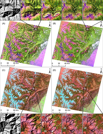
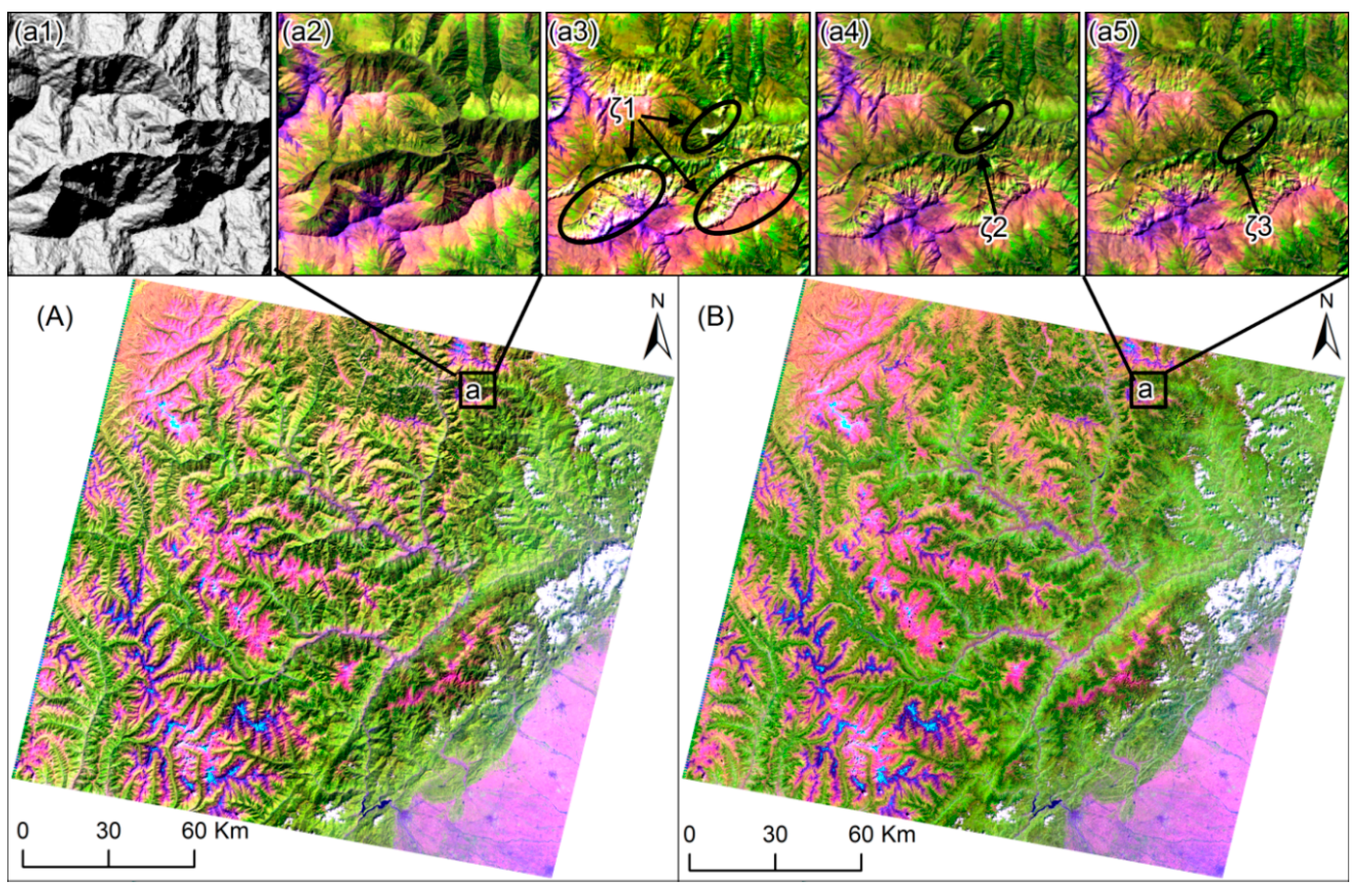
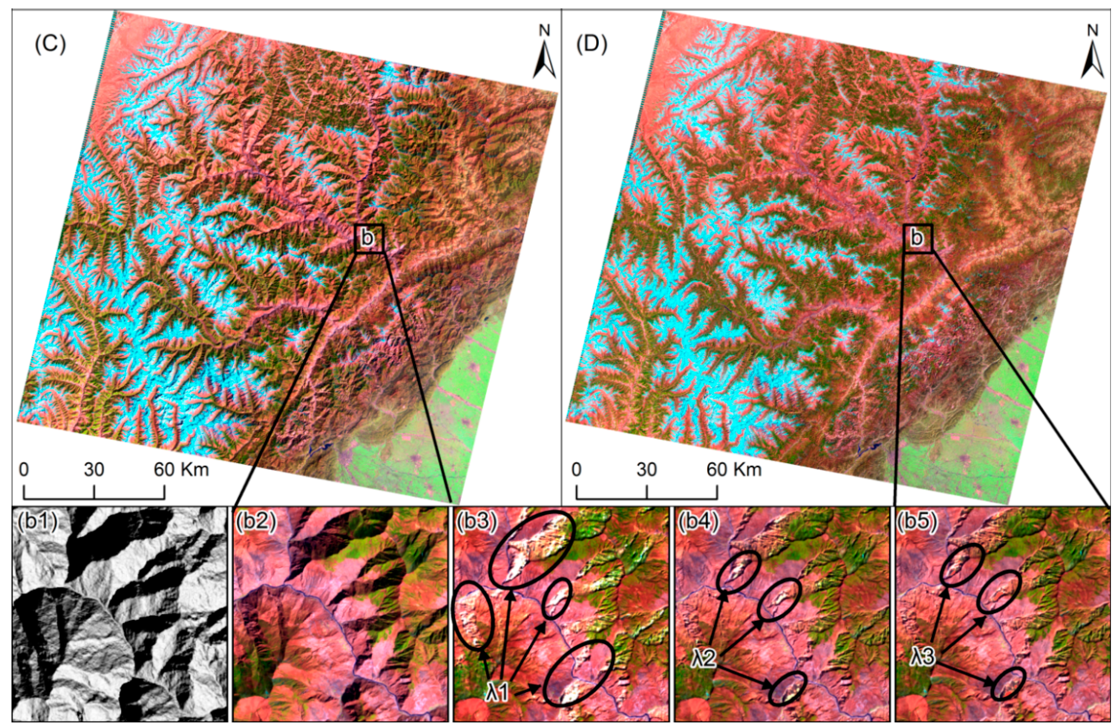
4.1. Visual Evaluation

Based on the improved model presented in this paper, two Landsat-5 TM images (referred to as spring scene and autumn scene, respectively) acquired under different solar elevation angles were processed. The topographic correction effects were evaluated by comparing both with the original image (after atmospheric correction, serve as benchmark) and correction results from Sandmeier model (representative of models with Lambertian assumption) and Li model (representative of models without Lambertian assumption). Figure 2 shows the overall visual effect of the two TM scenes, both before and after topographic correction. Also, smaller sub-scenes in typical areas with large variations of topography were chosen and enlarged to reveal the subtle differences of correction results by different methods. It can be seen from Figure 2B,D that topographic effects were greatly suppressed after correction, with reflectance in sun-averted slopes being evidently enhanced and information in shaded areas being recovered. Reflectance of the same land cover type on sun-facing and sun-averted slopes became much more identical, and overall quality of the images were significantly improved. Moreover, the proposed model performed consistently well for both spring and autumn images.

Performances of the three models were quite similar in gentle-slope areas. However, notable distinctions existed for severely rugged areas. From the illumination condition maps (a1 and b1) for the enlarged windows, we may partly feel the considerable ruggedness in chosen areas. Fairly serious overcorrection can be seen in faintly-illuminated area corrected by Sandmeier model (ζ1 in a3 and λ1 in b3). This may be owing to the Lambertian assumption in Sandmeier model, which simplifies the anisotropic scattering behavior of land surface. And this simplification does not impact correction result too much with low incident angles, while it leads to large discrepancy from reality with high incident angles; this is consistent with Richter’s conclusion [4]. Compared with Sandmeier model, Li model reduced the overcorrection to a large extent (a4 vs. a3, b4 vs. b3), by roughly considering the land surface BRDF effect. Model proposed in this paper slightly outperformed Li model (ζ2 in a4 vs. ζ3 in a5, λ2 in b4 vs. λ3 in b5) and further reduced the overcorrection phenomenon. Nevertheless, the visually detectable improvements of correction results from model proposed, when compared with that from Li model, mainly come from the over-correction adjustment of the shadow areas. The improvements for other areas are minor and inconspicuous, and hard to detect by visual evaluation. However, the improvements can be confirmed by the following quantitative analysis.

Figure 2. TM scenes before and after topographic correction (composite of band 5, 4 and 3 in red, green and blue), the upper half part is for the autumn scene, and the lower for the spring scene. (A) is autumn scene before correction; (B) after correction by the proposed model; (a1) is illumination condition map for “sub-scene a”; (a2) is enlarged window for “sub-scene a”; (a3–a5) are “sub-scene a” corrected by Sandmeier model, Li model and model proposed, respectively; (C) is spring scene before correction; (D) after correction by the proposed model; (b1) is illumination condition map for “sub-scene b”; (b2) is enlarged window for “sub-scene b”; and (b3–b5) are “sub-scene b” corrected by Sandmeier model, Li model and the proposed model, respectively.

Figure 2. TM scenes before and after topographic correction (composite of band 5, 4 and 3 in red, green and blue), the upper half part is for the autumn scene, and the lower for the spring scene. (A) is autumn scene before correction; (B) after correction by the proposed model; (a1) is illumination condition map for “sub-scene a”; (a2) is enlarged window for “sub-scene a”; (a3–a5) are “sub-scene a” corrected by Sandmeier model, Li model and model proposed, respectively; (C) is spring scene before correction; (D) after correction by the proposed model; (b1) is illumination condition map for “sub-scene b”; (b2) is enlarged window for “sub-scene b”; and (b3–b5) are “sub-scene b” corrected by Sandmeier model, Li model and the proposed model, respectively.

4.2. Statistical Analysis

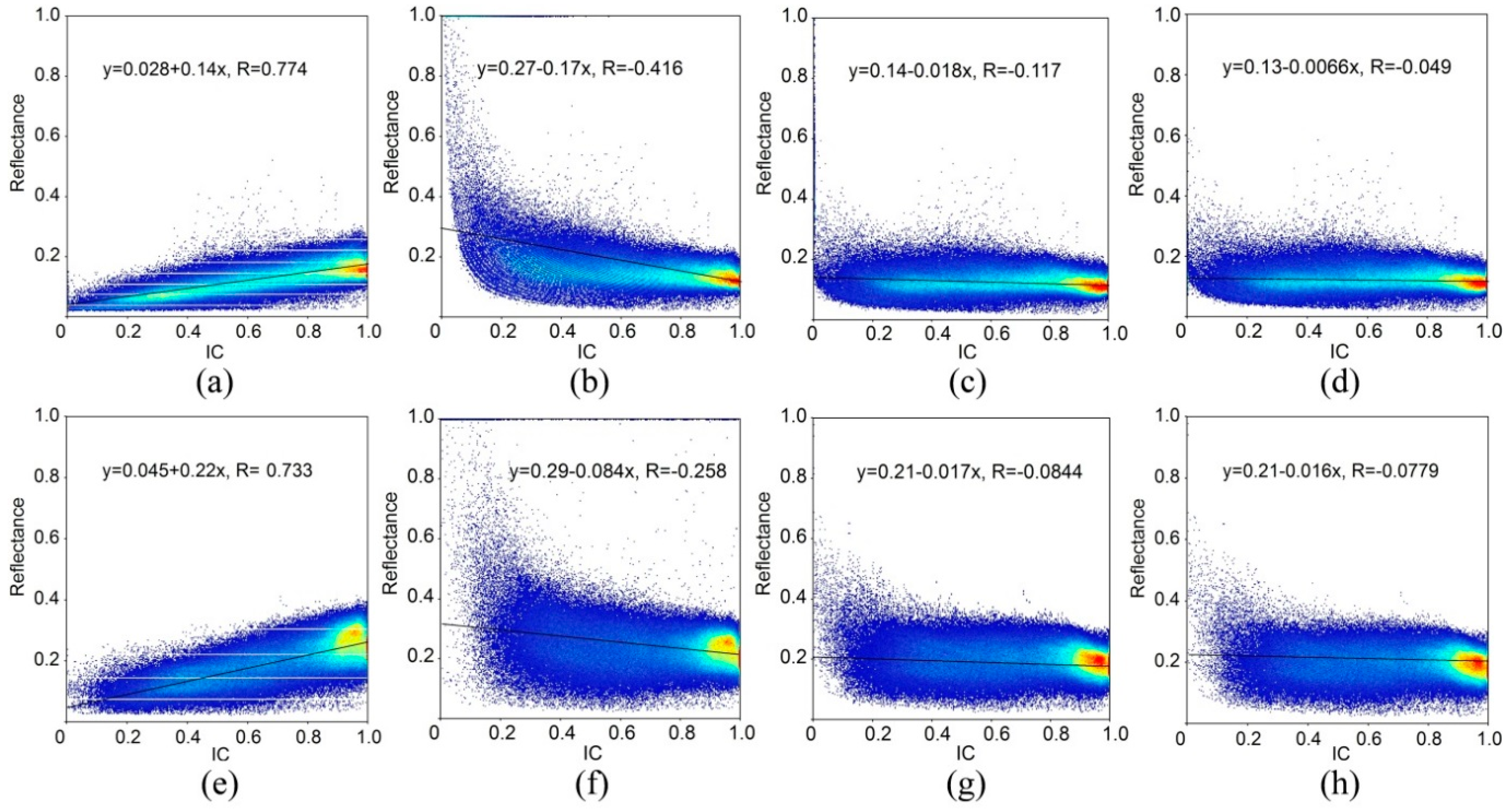
4.2.1. Reflectance Analysis

To further investigate the overall reflectance change for different slopes and aspects after topographic correction, we took band 4 for instance and demonstrated the reflectance intensity distribution of each sub-scene outlined in Figure 2 with polar-coordinate plots (Figure 3). The upper row is for the original spring TM sub-scene and its correction results by different methods; the lower row is for the autumn TM sub-scene and its corresponding correction results. It is evident that sun-facing slopes (aspect angles ranging from about 49° to about 229°) reveal higher reflectance values than sun-averted slopes before topographic correction, though the land cover types are quite uniformly distributed in terms of slopes and aspects (as can be seen in Figure 2). This phenomenon, if not being dealt with, is expected to interfere with the subsequent application of images.

Figure 3. The reflectance intensity distribution of band 4 from different topographic correction methods for different slope (denoted by the radius) and aspect angles (a–h). The upper row is the for spring TM sub-scene and its correction results from different methods; the lower row is for the autumn TM sub-scene and its correction results from different methods, therein, first column for the original images, second column for the correction results by Sandmeier model, third column for the correction results by Li model, forth column for the correction results by the model proposed, respectively.

Figure 3. The reflectance intensity distribution of band 4 from different topographic correction methods for different slope (denoted by the radius) and aspect angles (a–h). The upper row is the for spring TM sub-scene and its correction results from different methods; the lower row is for the autumn TM sub-scene and its correction results from different methods, therein, first column for the original images, second column for the correction results by Sandmeier model, third column for the correction results by Li model, forth column for the correction results by the model proposed, respectively.

After topographic correction by Sandmeier model, reflectance in sun-averted slopes is strongly enhanced, and the reflectance values tend to be more uniformly distributed than before. However, some points in sun-averted slopes (with relatively large slope angles) show inharmonious large values, especially for the spring sub-scene (Figure 3b). This may be explained by the over-correction of faintly illuminated pixels. Li model and model proposed achieved very similar results (Figure 3c vs. Figure 3d, Figure 3g vs. Figure 3h). They all further reduced the reflectance differences between sun-facing and sun-averted slopes, and made the reflectance distribution more uniform compared with Sandmeier model. Minor differences between results from Li model and model proposed are not directly noticeable. Thus, subtractions between them were done and demonstrated in Figure 4. Nevertheless, Figure 4 only suggests that differences exist. Whether proposed model outperforms Li model need further quantitative investigation.

Figure 4. Reflectance intensity differences of band 4 between results from model proposed and Li model, (a) for the spring scene, and (b) for the autumn scene.

Figure 4. Reflectance intensity differences of band 4 between results from model proposed and Li model, (a) for the spring scene, and (b) for the autumn scene.

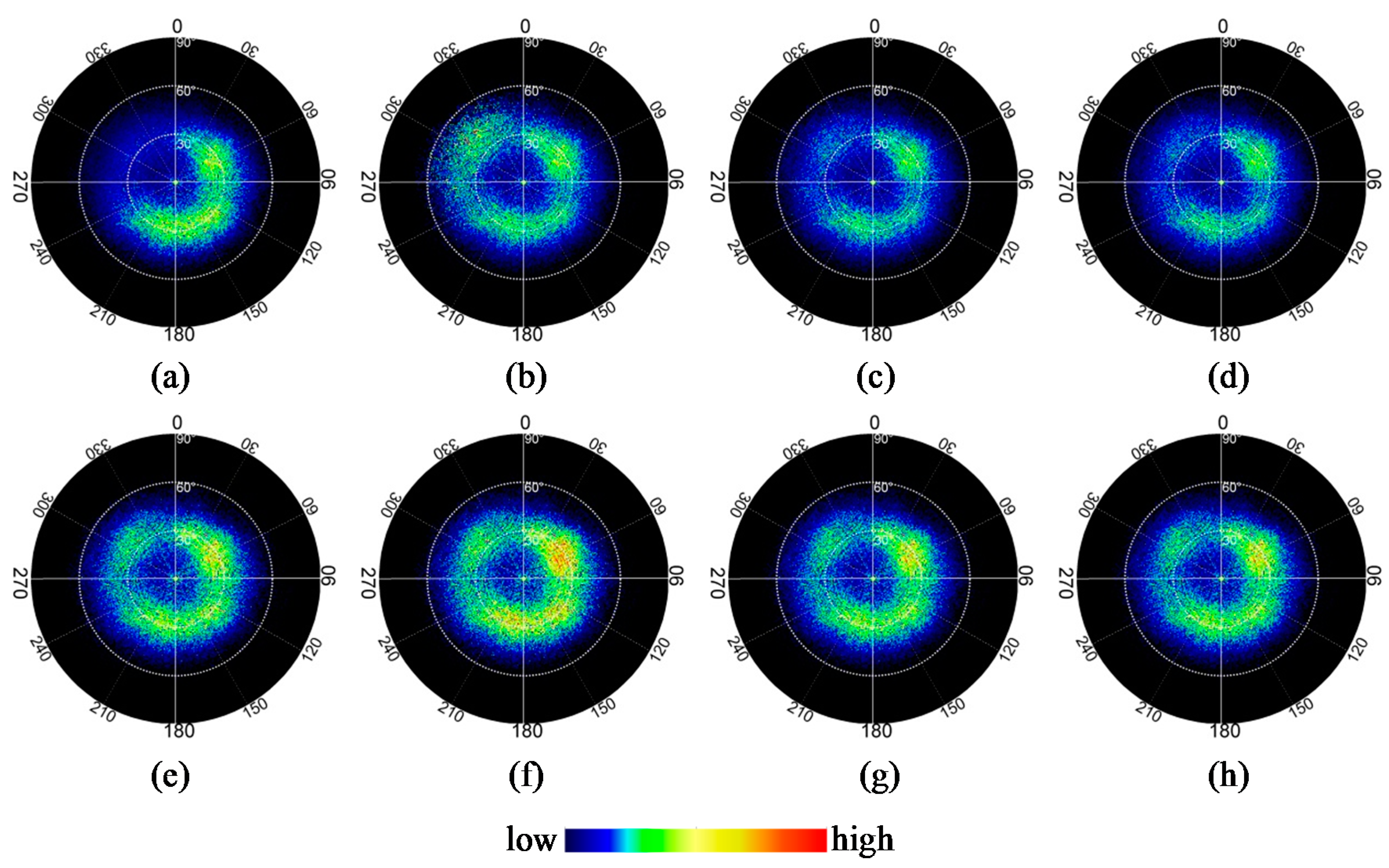
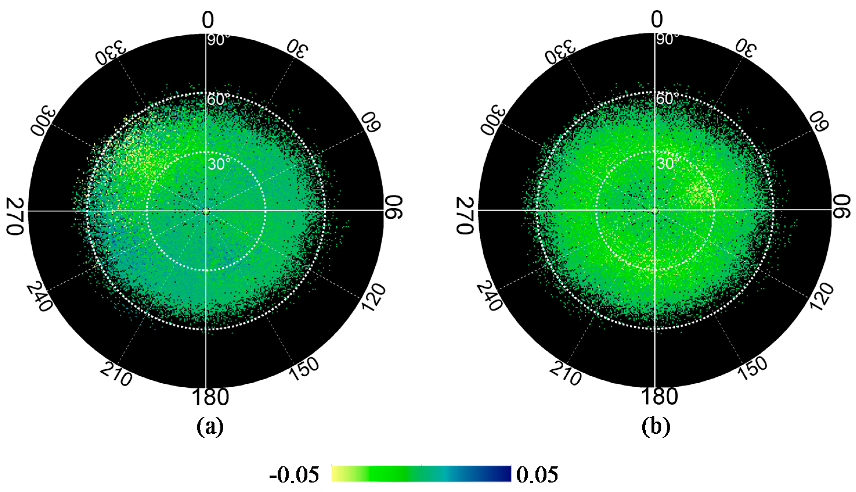
4.2.2. De-Correlation Analysis

Surface reflectance of remotely sensed image in mountainous area is positively correlated with illumination condition (IC, cosine of the local incident angle) due to topographic effect [18,20]. Technically, the higher the correlation coefficient is, the stronger the terrain effect is. Thus, the residual correlation is commonly examined to quantitatively indicate whether or to what extent the topographic effects still exist after topographic correction [18,20]. (It is noteworthy that aspect-related correlation between reflectance and illumination condition may remain after fully topographic correction, and this will be discussed in the Discussion Section.) Near infrared (NIR) band is suggested to be used, because it is less influenced by atmospheric scattering than visible bands [4]. Figure 5 demonstrates scatter plots between reflectance and IC for the two TM scenes both before and after topographic correction by different models, respectively. Before plots being drawn, invalid reflectance pixels (negative reflectance resulting from atmospheric overcorrection), cloud and cloud shadow pixels were screened out.

Before correction, as can be seen from Figure 5a,e, the reflectance shows a strong linear correlation with IC. The points are uniformly distributed in both sides of the fitted line, and correlation coefficients between NIR reflectance and IC reach 0.774 and 0.733 for spring and autumn scene, respectively. It implies that original images were subject to quite serious topographic effects. After topographic correction with different methods, correlation coefficients decreased to different levels. Among them, the proposed model in this paper always gained the lowest absolute value of correlation coefficients (−0.049 and −0.0779), which are very close to zero. For results from Li model, the correlation coefficients are −0.117 and −0.084, a litter larger (in absolute value) than that from model proposed. Sandmeier model obviously performed the worst, with quite large negative coefficients (−0.416 and −0.258), indicating serious overcorrection. Moreover, it can be seen that the overcorrections mainly concentrate in the low IC value area, and the corresponding points almost form a “tail” shape (Figure 5b,f), which is consistent with the phenomenon seen in Figure 2. This may suggest that Lambertian assumption need to be discarded when performing terrain correction in complex mountainous region. Besides, according to some researches [19,30,53], slopes of the regression lines of the scatter plots are also important in indicating the topographic correction effects. From this point of view, the same conclusion for the model performances could also be drawn, since the slopes of regression lines before and after topographic correction show exactly the same variation trend with correlation coefficients (seen from equations in Figure 5).

Figure 5. Scatter plots between NIR band reflectance and illumination condition (IC). (a) is spring TM scene before correction; and (b–d) are correction results by Sandmeier model, Li model and model proposed, respectively. (e) is autumn TM scene before correction; and (f–h) are correction results by Sandmeier model, Li model and model proposed, respectively.

Figure 5. Scatter plots between NIR band reflectance and illumination condition (IC). (a) is spring TM scene before correction; and (b–d) are correction results by Sandmeier model, Li model and model proposed, respectively. (e) is autumn TM scene before correction; and (f–h) are correction results by Sandmeier model, Li model and model proposed, respectively.

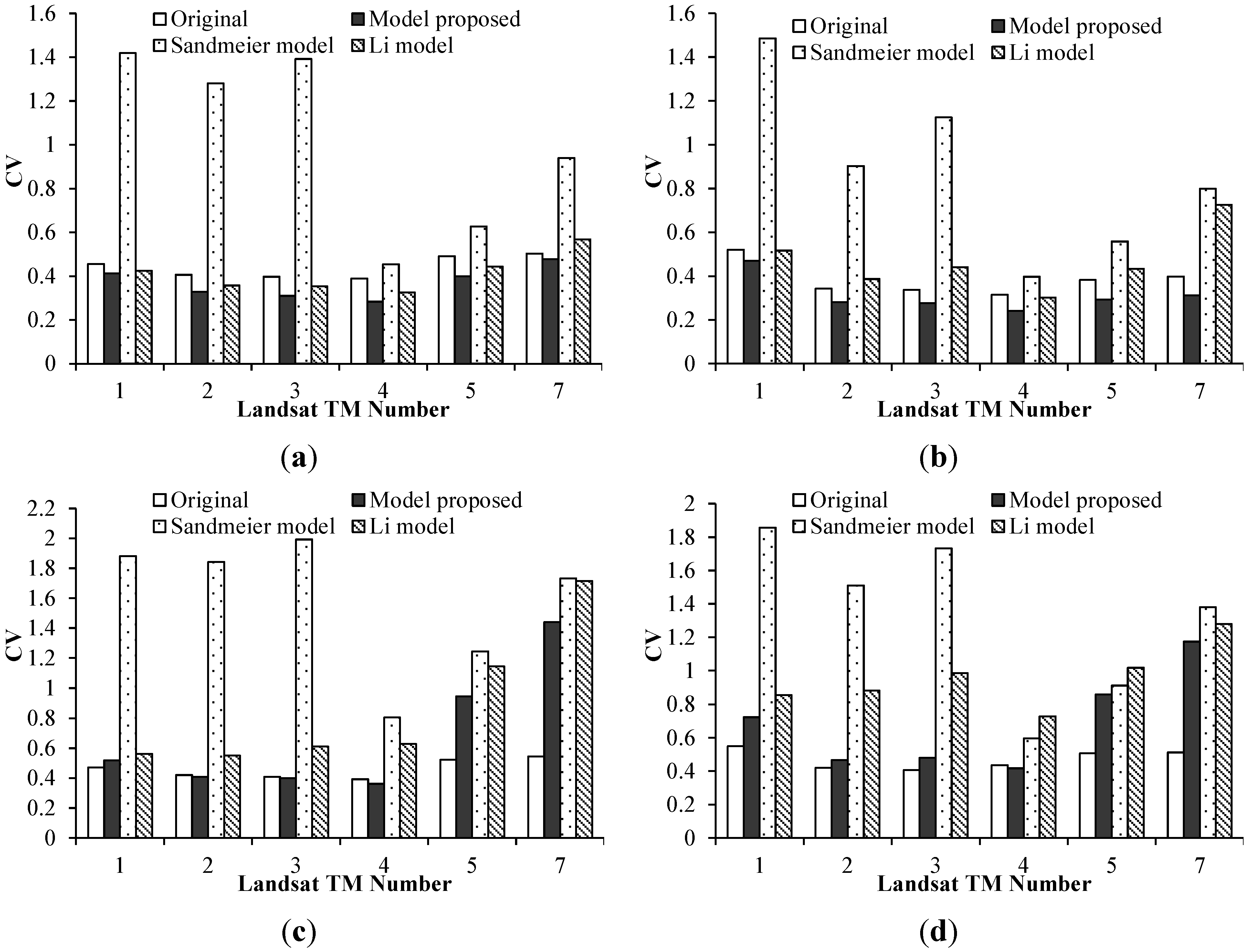
4.2.3. Coefficients of Variance

Coefficient of variance (CV), the ratio of standard deviation to the mean, is a statistical measure of the dispersion of data points. Theoretically, the CV of reflectance of the same land cover type will decrease due to much more consistency expected for the same land cover type from sun-facing and sun-averted slopes after successful topographic correction. Nevertheless, shadow areas, peculiarly prone to be over-corrected during topographic correction, may interfere and even conceal this trend when appraised together with the illuminated areas. Thus, we choose to evaluate the CVs of reflectance of the same land cover type for shadow areas and non-shadow areas separately. Also, by doing this, the improved model’s ability to topographically correct illuminated areas and shadow areas can be demonstrated more clearly. Forest pixels in shadow areas and non-shadow areas were extracted separately by referring to the land cover map and DEM-derived shadow mask of the study area. CVs of forest pixels (shadow and non-shadow areas separately) were calculated for each band of the reflectance before and after terrain correction by different models. For spring and autumn scenes, results are illustrated in Figure 6.

Figure 6. Coefficients of variance of forest pixels for each band before and after topographic correction by different models; (a) is for non-shadow forest of spring TM scene; (b) for non-shadow forest of autumn TM scene; (c) for shadow forest of spring TM scene; and (d) for shadow forest of autumn TM scene.

Figure 6. Coefficients of variance of forest pixels for each band before and after topographic correction by different models; (a) is for non-shadow forest of spring TM scene; (b) for non-shadow forest of autumn TM scene; (c) for shadow forest of spring TM scene; and (d) for shadow forest of autumn TM scene.

It can be seen from Figure 6a,b that degrees of CV alteration for illuminated forests after topographic correction vary obviously among different correction models. For Sandmeier model, the CVs increased for all bands (with visible bands exceptionally conspicuous) for both spring and autumn scenes. Serious overcorrection for steep areas with large incident/exiting angles, leading to extremely large reflectance values, may be responsible for this phenomenon. For spring scene (Figure 6a), Li model and model proposed all succeeded in decreasing CVs to some extent expect for band 7, and model proposed tended to slightly outperform Li model. For autumn scene (Figure 6b), Li model did not reduce the CVs except for band 4, while model improved could still decrease the CVs slightly for each band. Thus, model proposed seems to perform more stably in reducing the CVs for illuminated land covers, at least for forests.

Figure 6c,d shows the CVs of reflectance for shadowed forests before and after topographic correction. All models tended to increase the CVs, and only band 4 for spring and autumn scenes corrected by model proposed showed some minor reduction. Compared with the other two models, model proposed leaded to less increases of CVs for each band when 3 models all increased CVs. But, overall, topographic modeling for correction of shadow areas may be not enough for all three physics-based models, and modifications for the models are still needed.

5. Discussion

Mountain ecosystem protection and mountain development hold great significance to global human community [2]. Remote sensing plays an irreplaceable and important role in monitoring mountain areas on a regular basis, especially for those spatially inaccessible areas with highly heterogeneous and complex land covers. However, topographic undulation modifies the configuration of STS geometry as well as solar irradiance reaching the surface, and makes topographic distortion and BRDF effect pronounced in remotely sensed images. This challenging problem hampers the quantitative application of remote sensing and proves to be rather serious in moderate and high-resolution imagery, like Landsat-5 TM images. More and more researches show that it is necessary to solve this problem without the Lambertian assumption [18,19,20]. However, Landsat-5 TM provides scarce multi-angular observations to enable the extraction of BRDF information, and other data sources of matching BRDF information for the land surface are not readily available. In literature [20], Li et al. (2012) applied 500 m resolution MODIS BRDF parameters to account for the BRDF effect in corresponding TM images, and achieved satisfactory results. Nevertheless, averaging BRDF parameters over the whole TM scene and using the same BRDF shape function for all the land cover types may need further discussion when non-homogeneous mountainous areas are considered. Flood (2013) pointed out that MODIS BRDF parameters could only serve to provide a general, average correction for BRDF effects in Landsat TM imagery, and they do not carry any further information about BRDF effects on each Landsat pixel [54]. Thus, model presented in this paper, instead of using MODIS BRDF parameters for corresponding TM pixels, employed NDVI thresholds to divide land targets into eleven groups and each group used its own averaged BRDF parameters, and it had been experimented on Landsat TM images acquired under different sun elevation angles and shown to further improve the topographic correction effect. Nevertheless, some critical points still need further discussion.

Figure 7. Correlation coefficients between reflectance and illumination condition for different aspect intervals before and after topographic correction; (a) is for the whole spring scene; and (b) for forest in spring scene.

Figure 7. Correlation coefficients between reflectance and illumination condition for different aspect intervals before and after topographic correction; (a) is for the whole spring scene; and (b) for forest in spring scene.

In this paper, correlation between image reflectance and IC was applied to quantitatively indicate the topographic correction effect. Since the imaging process of sensors aboard satellite is quasi-instantaneous, the direction of solar illumination depicted by solar zenith and azimuth angles during the image acquisition is unique. The aim of topographic correction is to model the process and compensate for the unevenly distributed sunlight, induced by instant and unidirectional solar illumination and terrain ruggedness, which leads to distortion of radiance and reflectance. Thus, image reflectance after successful correction is expected to show almost no correlation with the instantaneous illumination condition, as demonstrated in Figure 5. However, in the long term, the land covers, especially vegetation, do show some correlation with slope orientation, because of the aspect-related differences in abiotic conditions [55,56,57], like moisture and temperature. Theoretically, aspect-related correlation between reflectance and illumination condition still exists even after successful topographic correction. To prove that, aspect angles of terrain were divided into eight intervals, with resolution of 45 degrees. Then, taking spring TM scene for instance, correlation between NIR band reflectance and IC before and after correction was examined for each aspect interval. For the whole image (Figure 7a), correlation coefficient reached maximum of about 0.35 for Northwest and West aspect intervals before correction, while only 0.05 for South and East intervals. After topographic correction by Li model and the proposed improved model, correlations decreased except for East, Southeast and South intervals. This implies reflectance still correlates with IC to various extents for different aspect intervals, though topographic correction has successfully removed the impacts by unidirectional illumination for the whole image scene. The same were examined and presented for forest pixels solely in Figure 7b. Correlation also reached maximum (0.4) in Northwest interval, and remained about 0.25 for other intervals before correction. They decreased to about 0.1 for almost all intervals after topographic correction by Li model and model proposed. This implies subtle correlation still exists between forest reflectance and IC for each aspect interval, which may be attributed to the insufficient topographic correction or the influence on vegetation growth states by abiotic factors [58].

Model improved in this paper employs MODIS BRDF products as ancillary data to account for the anisotropic behavior of surface reflectance recorded in TM images. It provides methodology of considering BRDF effects in topographic correction for moderate and high-resolution images. However, spatial resolution difference may impact the topographic correction effects to some extent. A MODIS pixel with nominal resolution of 500m at nadir (corresponding to about 278 TM pixels) is often mixture of different land cover types in TM scene [59]. Though linear additive kernel-driven model is applied to generate MCD43A1 products, reflectance of natural land targets in real scene may not simply be represented by the sum of products of end-member reflectance and corresponding area [60], taking into account the topographic relief and mutual-shadowing effect. This will potentially influence the model’s ability to reduce topographic effect. Apart from this, Flood reported (2013) that MODIS BRDF parameters may capture no local information about BRDF effect on TM pixel scale due to their large resolution difference [54]. Though the report is based on the tests solely performed on rather flat areas, it may be also the case in rugged areas. For mountainous areas, the angular configurations of the sun and sensor relative to the land target vary more severely. Therefore, much bigger part of the BRDF shape being modeled by the MODIS BRDF processing will be necessary when using MODIS BRDF parameters to account for BRDF effect in mountainous TM images. This is not like the situation in which only a very small part (mostly central part, near nadir) of the BRDF shape is used for BRDF correction of TM images of flat areas, as described by Flood. Thus, uncertainties of employing MODIS BRDF parameters to account for angular effect in Landsat TM imagery still exist and need further research. In the future, it is anticipated that BRDF information matching TM spatial resolution will be derived from satellite constellations with short revisit cycle and multi-angular viewing ability, like China’s HJ-1 A/B [61,62] and the forthcoming European Space Agency (ESA)’s Sentinel-2A/B [63,64]. It will be advisable to interpret BRDF effect in TM scenes using matching BRDF data. Besides, bandwidths of MODIS images are narrower than corresponding TM ones and their spectral response functions differ, which may also potentially affect the accuracy of methodology proposed [24].

Typically, there will be several land cover types in the domain of a TM scene as to mountain ecosystem. For instance, TM scenes covering the study area selected in this paper include forests, shrubs, grasslands, cultivated lands, residential lands and barrens (Figure 1b). Different land covers usually show different BRDF effects [65,66], which should be considered in topographic correction. However, the availability of matching and precise BRDF information and land cover map is restricted. Some researchers attempted to use the average BRDF shape function for the whole study area when conducting topographic correction, and meanwhile, pointed out the necessity of employing different BRDF shape functions for different land cover types [20]. Model improved in this paper divides the land targets into eleven groups with NDVI thresholds, and uses different BRDF model parameters to perform topographic correction for different group of targets, which helps to account for the surface anisotropy more effectively [65]. It can be seen from Table 1 that the BRDF shape function parameters for different NDVI intervals of each band have apparent differences. Since NDVI is the ratio of simple band by algebraic operation, it is capable of restraining topographic effect compared to single band [47]. Moreover, NDVI can approximately indicate land cover types, and is readily available compared to other ancillary land cover data. These merits make model improved in this paper widely effective, practicable and potentially operational. Nevertheless, it is noteworthy that NDVI alone cannot distinguish dense vegetation types or non-vegetated areas. This is a big limitation our model encounters, and further thoughts are required to overcome it.

ASTER GDEM (version 2) is employed to depict the rugged land surface and derive terrain factors, like slope and aspect, which serve as crucial input parameters for topographic correction. ASTER GDEM is produced with optical stereo pixel pairs, and it is prone to being impacted by cloud and mist (especially in mountainous areas), though version 2 improves on quality against version 1. Bian et al. (2013) concluded that evident noise exists in ASTER GDEM for some local mountainous regions, though it is more capable of revealing details than SRTM [67]. Nan et al. (2014) reported that the overall horizontal accuracy of ASTER GDEM is better than that of SRTM in eastern Qinghai-Tibetan Plateau, but the opposite is the case for the overall vertical accuracy [25]. Since accuracy of DEM has a significant influence on topographic correction effect, some researchers have explored and given suggestions on what resolution of DEM is appropriate for topographic correction. Gao et al. (2009) claimed that the same resolution is enough to achieve satisfactory correction results [53]. Hantson et al. (2011) suggested that resolution of DEM used should be one third of that of images to be corrected [14]. Zhang et al. (2015) even concluded that 30-m DEM can only satisfy the correction of 90- to 500-m resolution remote sensing images [68]; this question still needs further and systematic investigations. Apart from that, local artifacts or noises in DEM also impact the correction effect, and this is expected to be suppressed by filtering of DEM prior to topographic correction. Nevertheless, it should be noted that DEM filtering modifies the original values and may potentially reduce the quantitative accuracy of remote sensing.

In the procedure of land surface remote sensing, the signals received by the satellite sensors are coupled and integrated results from atmosphere and land surface [38]. And this is especially true for the mountainous areas where the interactions between signals and land surface-atmosphere system are much more complicated. Therefore, the combined atmospheric and topographic correction methodologies are adopted by many researchers to remove the radiometric distortions of optical satellite images in mountain areas [5,18,19,20]. Vanonckelen et al. (2013, 2014) showed that coupled correction methods showed most efficiency on weakly illuminated slopes [30,69]. Li et al. (2012) also pointed out the strengths of combined methodology [20]. In this study, the improved model also corrects atmospheric and topographic effects simultaneously. However, we mainly modify the topographic correction module, and aim to see whether it works to improve the overall correction results. Thus, we evaluate the topographic correction effect separately, and make the atmospherically-corrected reflectance serve as the baseline scenario. Nevertheless, special emphasis should be put on the advantages of combined correction methodologies.

The interfering effect of topography is evident in a single satellite scene and introduces even stronger distortions in multi-temporal approaches [5]. Multi-temporal studies require a previous radiometric homogenization of input images to better identify true changes, and topographic correction is one of the key steps to produce consistent and radiometrically stable multi-temporal time series [14]. In this study, the improved model possesses a solid physical base and successfully avoids the scene-dependent empirical regression. Also, the BRDF effects are accounted for when performing topographic correction. All these attributes favor the radiometric correction for time series images and tend to promise a much higher accuracy on quantitative applications of multi-temporal or multi-sensor images [70].

The execution speed of the algorithm is also an important factor to be considered when automatically processing a tremendously large volume of imagery in near-real time is a necessity [71]. In this study, the spring TM scene contains 8051 × 7151 pixels (column × line), and the autumn scene contains 8031 × 7151 pixels. The processing time needed for each scene is about 11 hours on a typical personal computer (configuration: Inter(R) Core(TM) i7-3770 CUP @ 3.40GHz, and 4 GB memory). Efforts will be put into enhancing the algorithm to further shorten the processing time in the future.

6. Conclusions

Optical remotely sensed images in mountainous areas are subject to distortions induced by topographic effect. It impacts accuracy of image applications in various fields such as biophysical parameter inversion, time series data analysis and change detection to a large extent. Especially when time series images are employed for seasonal change information extraction, topography-induced reflectance distortion may mix with and even obscure the real seasonal changes. Thus, topographic correction is a preliminary and necessary step for image quantitative application. This paper proposed an improved physics-based topographic correction model under consideration of anisotropic behavior of surface scattering. Direct and diffuse solar irradiance and neighboring terrain irradiance received by rugged surfaces are computed based on 6S radiative transfer model and Hay model. NDVI thresholds are utilized to divide land targets into eleven groups, and each group employs corresponding averaged MODIS BRDF model parameters to solve the equations and gain the corrected reflectance. Topographic correction model proposed was tested with two Landsat-5 TM scenes of severely rugged mountainous areas acquired under different sun elevation angles, and compared with Sandmeier model (representative of models with Lambertian assumption) and Li model (representative of models without Lambertian assumption). Experiment results showed that model proposed performed very well, with reflectance in sun-averted slopes being enhanced and topographic effects being greatly suppressed. Also, correlation coefficients between NIR band reflectance and illumination condition reduced almost to zero, and coefficients of variance for illuminated forests decreased. Nevertheless, there are still some sources of uncertainty for the model proposed here. For instance, the model relies on MODIS BRDF products to account for the non-Lambertian property of land surface, and the accuracy of topographic correction depends largely on MODIS BRDF model parameters and DEM. Along with the development of high spatial and temporal resolution images, such as images from HJ-1 A/B and Sentinel-2 A/B, some of these problems may be solved, and the model proposed here may be further modified and operationally employed in the future.

References

1. Li, W. Global significance of mountain sustainable development. World For. Res. 2004, 17, 5–10. (in Chinese). [Google Scholar]
2. Grêt-Regamey, A.; Brunner, S.H.; Kienast, F. Mountain ecosystem services: Who cares? Mt. Res. Dev. 2012, 32, S23–S34. [Google Scholar] [CrossRef]
3. Colby, J.D. Topographic normalization in rugged terrain. Photogramm. Eng. Remote Sens. 1991, 57, 531–537. [Google Scholar]
4. Richter, R. Correction of satellite imagery over mountainous terrain. Appl. Opt. 1998, 37, 4004–4015. [Google Scholar] [CrossRef] [PubMed]
5. Sandmeier, S.; Itten, K.I. A physically-based model to correct atmospheric and illumination effects in optical satellite data of rugged terrain. IEEE Trans. Geosci. Remote Sens. 1997, 35, 708–717. [Google Scholar] [CrossRef]
6. Minnaert, M. The reciprocity principle in lunar photometry. Astrophys. J. 1941, 93, 403–410. [Google Scholar] [CrossRef]
7. Schaepman-Strub, G.; Schaepman, M.E.; Painter, T.H.; Dangel, S.; Martonchik, J.V. Reflectance quantities in optical remote sensing-definitions and case studies. Remote Sens. Environ. 2006, 103, 27–42. [Google Scholar] [CrossRef]
8. Li, A.; Jiang, J.; Bian, J.; Deng, W. Combining the matter element model with the associated function of probability transformation for multi-source remote sensing data classification in mountainous regions. ISPRS J. Photogramm. Remote Sens. 2012, 67, 80–92. [Google Scholar] [CrossRef]
9. Chen, J.; Chen, X.; Ju, W. Effects of vegetation heterogeneity and surface topography on spatial scaling of net primary productivity. Biogeosciences 2013, 10, 4879–4896. [Google Scholar] [CrossRef]
10. Gu, D.; Gillespie, A. Topographic normalization of Landsat TM images of forest based on subpixel sun-canopy-sensor geometry. Remote Sens. Environ. 1998, 64, 166–175. [Google Scholar] [CrossRef]
11. Soenen, S.A.; Peddle, D.R.; Coburn, C.A. SCS+C: A modified sun-canopy-sensor topographic correction in forested terrain. IEEE Trans. Geosci. Remote Sens. 2005, 43, 2148–2159. [Google Scholar] [CrossRef]
12. Teillet, P.; Guindon, B.; Goodenough, D. On the slope-aspect correction of multispectral scanner data. Can. J. Remote Sens. 1982, 8, 84–106. [Google Scholar] [CrossRef]
13. Ediriweera, S.; Pathirana, S.; Danaher, T.; Nichols, D.; Moffiet, T. Evaluation of different topographic corrections for Landsat TM data by prediction of foliage projective cover (FPC) in topographically complex landscapes. Remote Sens. 2013, 5, 6767–6789. [Google Scholar] [CrossRef]
14. Hantson, S.; Chuvieco, E. Evaluation of different topographic correction methods for Landsat imagery. Int. J. Appl. Earth Obs. 2011, 13, 691–700. [Google Scholar] [CrossRef]
15. Duan, S.; Yan, G. A review of models for topographic correction of remotely sensed images in mountainous area. J. Beijing Norm. Univ. (Nat. Sci.) 2007, 43, 362–366. [Google Scholar]
16. Richter, R.; Kellenberger, T.; Kaufmann, H. Comparison of topographic correction methods. Remote Sens. 2009, 1, 184–196. [Google Scholar] [CrossRef] [Green Version]
17. Gao, Y.; Zhang, W. A simple empirical topographic correction method for ETM+ imagery. Int. J. Remote Sens. 2009, 30, 2259–2275. [Google Scholar] [CrossRef]
18. Shepherd, J.D.; Dymond, J.R. Correcting satellite imagery for the variance of reflectance and illumination with topography. Int. J. Remote Sens. 2003, 24, 3503–3514. [Google Scholar] [CrossRef]
19. Wen, J.; Liu, Q.; Liu, Q.; Xiao, Q.; Li, X. Parametrized BRDF for atmospheric and topographic correction and albedo estimation in Jiangxi rugged terrain, China. Int. J. Remote Sens. 2009, 30, 2875–2896. [Google Scholar] [CrossRef]
20. Li, F.; Jupp, D.L.B.; Thankappan, M.; Lymburner, L.; Mueller, N.; Lewis, A.; Held, A. A physics-based atmospheric and BRDF correction for Landsat data over mountainous terrain. Remote Sens. Environ. 2012, 124, 756–770. [Google Scholar] [CrossRef]
21. Roy, D.P.; Wulder, M.; Loveland, T.; Woodcock, C.; Allen, R.; Anderson, M.; Helder, D.; Irons, J.; Johnson, D.; Kennedy, R.; et al. Landsat-8: Science and product vision for terrestrial global change research. Remote Sens. Environ. 2014, 145, 154–172. [Google Scholar] [CrossRef]
22. Tucker, C.J.; Grant, D.M.; Dykstra, J.D. NASA’s global orthorectified Landsat data set. Photogramm. Eng. Remote Sens. 2004, 70, 313–322. [Google Scholar] [CrossRef]
23. Chander, G.; Markham, B.L.; Helder, D.L. Summary of current radiometric calibration coefficients for Landsat MSS, TM, ETM+, and EO-1 ALI sensors. Remote Sens. Environ. 2009, 113, 893–903. [Google Scholar] [CrossRef]
24. Li, F.; Jupp, D.L.B.; Reddy, S.; Lymburner, L.; Mueller, N.; Tan, P.; Islam, A. An evaluation of the use of atmospheric and BRDF correction to standardize Landsat data. IEEE J. Sel. Top. Appl. Earth Obs. 2010, 3, 257–270. [Google Scholar] [CrossRef]
25. Nan, X.; Li, A.; Bian, J.; Zhang, Z. Comparison of the accuracy between SRTM and ASTER GDEM over typical mountainous area: A case study in the eastern Qinghai-Tibetan Plateau. J. Geo-Inf. Sci. 2014, 1, 1. (in Chinese). [Google Scholar]
26. Wechsler, S.P.; Kroll, C.N. Quantifying DEM uncertainty and its effect on topographic parameters. Photogramm. Eng. Remote Sens. 2006, 72, 1081–1090. [Google Scholar] [CrossRef]
27. Huang, H.; Gong, P.; Clinton, N.; Hui, F. Reduction of atmospheric and topographic effect on Landsat TM data for forest classification. Int. J. Remote Sens. 2008, 29, 5623–5642. [Google Scholar] [CrossRef]
28. Nichol, J.; Hang, L.K. The influence of DEM accuracy on topographic correction of Ikonos satellite images. Photogramm. Eng. Remote Sens. 2008, 74, 47–53. [Google Scholar] [CrossRef]
29. Riaño, D.; Chuvieco, E.; Salas, J.; Aguado, I. Assessment of different topographic corrections in Landsat-TM data for mapping vegetation types. IEEE Trans. Geosci. Remote Sens. 2003, 41, 1056–1061. [Google Scholar] [CrossRef]
30. Vanonckelen, S.; Lhermitte, S.; Balthazar, V.; van Rompaey, A. Performance of atmospheric and topographic correction methods on Landsat imagery in mountain areas. Int. J. Remote Sens. 2014, 35, 4952–4972. [Google Scholar] [CrossRef]
31. Hirt, C.; Filmer, M.; Featherstone, W. Comparison and validation of the recent freely available ASTER-GDEM ver1, SRTM ver4. 1 and GEODATA DEM-9S ver3 digital elevation models over Australia. Aust. J. Earth Sci. 2010, 57, 337–347. [Google Scholar] [CrossRef]
32. Jiang, K.; Zhao, Y.; Geng, X.; Tang, H. Topographic correction of ETM images based on smoothed terrain. J. Electron. (China) 2012, 29, 271–278. [Google Scholar] [CrossRef]
33. Roy, D.P.; Ju, J.; Lewis, P.; Schaaf, C.; Gao, F.; Hansen, M.; Lindquist, E. Multi-temporal MODIS-Landsat data fusion for relative radiometric normalization, gap filling, and prediction of Landsat data. Remote Sens. Environ. 2008, 112, 3112–3130. [Google Scholar] [CrossRef]
34. Wanner, W.; Strahler, A.; Hu, B.; Lewis, P.; Muller, J.P.; Li, X.; Schaaf, C.; Barnsley, M. Global retrieval of bidirectional reflectance and albedo over land from EOS MODIS and MISR data: Theory and algorithm. J. Geophys. Res.: Atmos. 1997, 102, 17143–17161. [Google Scholar] [CrossRef]
35. Strahler, A.H.; Muller, J.; Lucht, W.; Schaaf, C.; Tsang, T.; Gao, F.; Li, X.; Lewis, P.; Barnsley, M.J. MODIS BRDF/albedo Product: Algorithm Theoretical Basis Document Version 5.0. Available online: http://modis.gsfc.nasa.gov/data/atbd/atbd_mod09.pdf (accessed on 19 May 2014).
36. Schaaf, C.B.; Gao, F.; Strahler, A.H.; Lucht, W.; Li, X.W.; Tsang, T.; Strugnell, N.C.; Zhang, X.Y.; Jin, Y.F.; Muller, J.P.; et al. First operational BRDF, albedo nadir reflectance products from MODIS. Remote Sens. Environ. 2002, 83, 135–148. [Google Scholar] [CrossRef]
37. Li, A.; Lei, G.; Zhang, Z.; Bian, J.; Deng, W. China land cover monitoring in mountainous regions by remote sensing technology—Taking the southwestern China as a case. In Proceedings of 2014 IEEE International Geoscience and Remote Sensing Symposium (IGARSS 2014), Quebec, QC, Canada, 13–18 July 2014; pp. 4216–4219.
38. Hu, B.; Lucht, W.; Strahler, A.H. The interrelationship of atmospheric correction of reflectances and surface BRDF retrieval: A sensitivity study. IEEE Trans. Geosci. Remote Sens. 1999, 37, 724–738. [Google Scholar] [CrossRef]
39. Vermote, E.; El Saleous, N.; Justice, C.; Kaufman, Y.; Privette, J.; Remer, L.; Roger, J.; Tanre, D. Atmospheric correction of visible to middle-infrared EOS-MODIS data over land surfaces: Background, operational algorithm and validation. J. Geophys. Res.: Atmos. 1997, 102, 17131–17141. [Google Scholar] [CrossRef]
40. Pearson, F. Map Projections: Theory and Applications; CRC Press: Boca Raton, FL, USA, 1990; p. 372. [Google Scholar]
41. Hay, J.E. Calculation of solar irradiances for inclined surfaces: Validation of selected hourly and daily models. Atmos.-Ocean 1986, 24, 16–41. [Google Scholar] [CrossRef]
42. Liu, M.; Bárdossy, A.; Li, J.; Jiang, Y. GIS-based modelling of topography-induced solar radiation variability in complex terrain for data sparse region. Int. J. Geogr. Inf. Sci. 2012, 26, 1281–1308. [Google Scholar] [CrossRef]
43. Feng, M.; Sexton, J.O.; Huang, C.; Masek, J.G.; Vermote, E.F.; Gao, F.; Narasimhan, R.; Channan, S.; Wolfe, R.E.; Townshend, J.R. Global surface reflectance products from Landsat: Assessment using coincident MODIS observations. Remote Sens. Environ. 2013, 134, 276–293. [Google Scholar] [CrossRef]
44. Masek, J.G.; Vermote, E.F.; Saleous, N.E.; Wolfe, R.; Hall, F.G.; Huemmrich, K.F.; Gao, F.; Kutler, J.; Lim, T.-K. A Landsat surface reflectance dataset for North America, 1990–2000. IEEE Geosci. Remote Sens. Lett. 2006, 3, 68–72. [Google Scholar] [CrossRef]
45. Wanner, W.; Li, X.; Strahler, A.H. On the derivation of kernels for kernel-driven models of bidirectional reflectance. J. Geophys. Res.: Atmos. 1995, 100, 21077–21089. [Google Scholar] [CrossRef]
46. Jiao, Z.; Li, X.; Wang, J.; Zhang, H. Assessment of MODIS BRDF shape indicators. J. Remote Sens. 2011, 15, 432–456. [Google Scholar]
47. Zhu, G.; Liu, Y.; Ju, W.; Chen, J. Evaluation of topographic effects on four commonly used vegetation indices. J. Remote Sens. 2013, 17, 210–234. [Google Scholar]
48. Lucht, W.; Schaaf, C.B.; Strahler, A.H. An algorithm for the retrieval of albedo from space using semiempirical BRDF models. IEEE Trans. Geosci. Remote Sens. 2000, 38, 977–998. [Google Scholar] [CrossRef]
49. Giles, P.T. Remote sensing and cast shadows in mountainous terrain. Photogramm. Eng. Remote Sens. 2001, 67, 833–839. [Google Scholar]
50. Schulmann, T.; Katurji, M.; Zawar-Reza, P. Seeing through shadow: Modelling surface irradiance for topographic correction of Landsat ETM+ data. ISPRS J. Photogramm. Remote Sens. 2015, 99, 14–24. [Google Scholar] [CrossRef]
51. Zhou, Y.; Chen, J.; Guo, Q.; Cao, R.; Zhu, X. Restoration of information obscured by mountainous shadows through Landsat TM/ETM plus images without the use of DEM data: A new method. IEEE Trans. Geosci. Remote Sens. 2014, 52, 313–328. [Google Scholar] [CrossRef]
52. Shahtahmassebi, A.; Yang, N.; Wang, K.; Moore, N.; Shen, Z. Review of shadow detection and de-shadowing methods in remote sensing. Chin. Geogr. Sci. 2013, 23, 403–420. [Google Scholar] [CrossRef]
53. Gao, Y.; Zhang, W. LULC classification and topographic correction of Landsat-7 ETM+ imagery in the Yangjia River Watershed: The influence of DEM resolution. Sensors 2009, 9, 1980–1995. [Google Scholar] [CrossRef] [PubMed]
54. Flood, N. Testing the local applicability of MODIS BRDF parameters for correcting Landsat TM imagery. Remote Sens. Lett. 2013, 4, 793–802. [Google Scholar] [CrossRef]
55. Badano, E.I.; Cavieres, L.A.; Molina-Montenegro, M.A.; Quiroz, C. Slope aspect influences plant association patterns in the Mediterranean matorral of central Chile. J. Arid Environ. 2005, 62, 93–108. [Google Scholar] [CrossRef]
56. Joseph, S.; Reddy, C.S.; Pattanaik, C.; Sudhakar, S. Distribution of plant communities along climatic and topographic gradients in Mudumalai Wildlife Sanctuary (southern India). Biol. Lett. 2008, 45, 29–41. [Google Scholar]
57. Dorji, T.; Odeh, I.O.; Field, D.J. Vertical distribution of soil organic carbon density in relation to land use/cover, altitude and slope aspect in the eastern Himalayas. Land 2014, 3, 1232–1250. [Google Scholar] [CrossRef]
58. Wondie, M.; Teketay, D.; Melesse, A.; Schneider, W. Relationship between topographic variables and land cover in the Simen Mountains National Park, a world heritage site in northern Ethiopia. Int. J. Remote Sens. Appl. 2012, 2, 36–43. [Google Scholar]
59. Zhao, W.; Li, A. A downscaling method for improving the spatial resolution of AMSR-E derived soil moisture product based on MSG-SEVIRI data. Remote Sens. 2013, 5, 6790–6811. [Google Scholar] [CrossRef]
60. Roman, M.O.; Gatebe, C.K.; Schaaf, C.B.; Poudyal, R.; Wang, Z.; King, M.D. Variability in surface BRDF at different spatial scales (30 m–500 m) over a mixed agricultural landscape as retrieved from airborne and satellite spectral measurements. Remote Sens. Environ. 2011, 115, 2184–2203. [Google Scholar] [CrossRef]
61. Jiang, B.; Liang, S.; Townshend, J.R.; Dodson, Z.M. Assessment of the radiometric performance of Chinese HJ-1 satellite CCD instruments. IEEE J. Sel. Top. Appl. Earth Obs. 2013, 6, 840–850. [Google Scholar] [CrossRef]
62. Bian, J.; Li, A.; Jin, H.; Zhao, W.; Lei, G.; Huang, C. Multi-temporal cloud and snow detection algorithm for the HJ-1A/B CCD imagery of China. In Proceedings of 2014 IEEE International Geoscience and Remote Sensing Symposium (IGARSS 2014), Quebec, QC, Canada, 13–18 July 2014; pp. 501–504.
63. Baillarin, S.; Meygret, A.; Dechoz, C.; Petrucci, B.; Lacherade, S.; Tremas, T.; Isola, C.; Martimort, P.; Spoto, F. Sentinel-2 level 1 products and image processing performances. In Proceedings of 2012 IEEE International Geoscience and Remote Sensing Symposium (IGARSS 2012), Munich, Germany, 22–27 July 2012; pp. 7003–7006.
64. Drusch, M.; Del Bello, U.; Carlier, S.; Colin, O.; Fernandez, V.; Gascon, F.; Hoersch, B.; Isola, C.; Laberinti, P.; Martimort, P. Sentinel-2: ESA’s optical high-resolution mission for GMES operational services. Remote Sens. Environ. 2012, 120, 25–36. [Google Scholar] [CrossRef]
65. Bacour, C.; Breon, F.M. Variability of biome reflectance directional signatures as seen by POLDER. Remote Sens. Environ. 2005, 98, 80–95. [Google Scholar] [CrossRef]
66. Jiao, Z.; Hill, M.J.; Schaaf, C.B.; Zhang, H.; Wang, Z.; Li, X. An anisotropic flat index (AFX) to derive BRDF archetypes from MODIS. Remote Sens. Environ. 2014, 141, 168–187. [Google Scholar] [CrossRef]
67. Bian, J.; Li, A.; Jin, H.; Lei, G.; Huang, C.; Li, M. Auto-registration and orthorecification algorithm for the time series HJ-1A/B CCD images. J. Mt. Sci. 2013, 10, 754–767. [Google Scholar] [CrossRef]
68. Zhang, Y.; Yan, G.; Bai, Y. Sensitivity of topographic correction to the DEM spatial scale. IEEE Geosci. Remote Sens. Lett. 2015, 12, 53–57. [Google Scholar] [CrossRef]
69. Vanonckelen, S.; Lhermitte, S.; van Rompaey, A. The effect of atmospheric and topographic correction methods on land cover classification accuracy. Int. J. Appl. Earth Obs. 2013, 24, 9–21. [Google Scholar] [CrossRef]
70. Vanonckelen, S.; Lhermitte, S.; van Rompaey, A. The effect of atmospheric and topographic correction on pixel-based image composites: Improved forest cover detection in mountain environments. Int. J. Appl. Earth Obs. 2015, 35, 320–328. [Google Scholar] [CrossRef]
71. Roy, D.P.; Ju, J.; Kline, K.; Scaramuzza, P.L.; Kovalskyy, V.; Hansen, M.; Loveland, T.R.; Vermote, E.; Zhang, C. Web-enabled Landsat data (WELD): Landsat ETM+ composited mosaics of the conterminous United States. Remote Sens. Environ. 2010, 114, 35–49. [Google Scholar] [CrossRef]