
Downscaling 250-m MODIS Growing Season NDVI Based on Multiple-Date Landsat Images and Data Mining Approaches


Abstract
:
1. Introduction
2. Data and Method
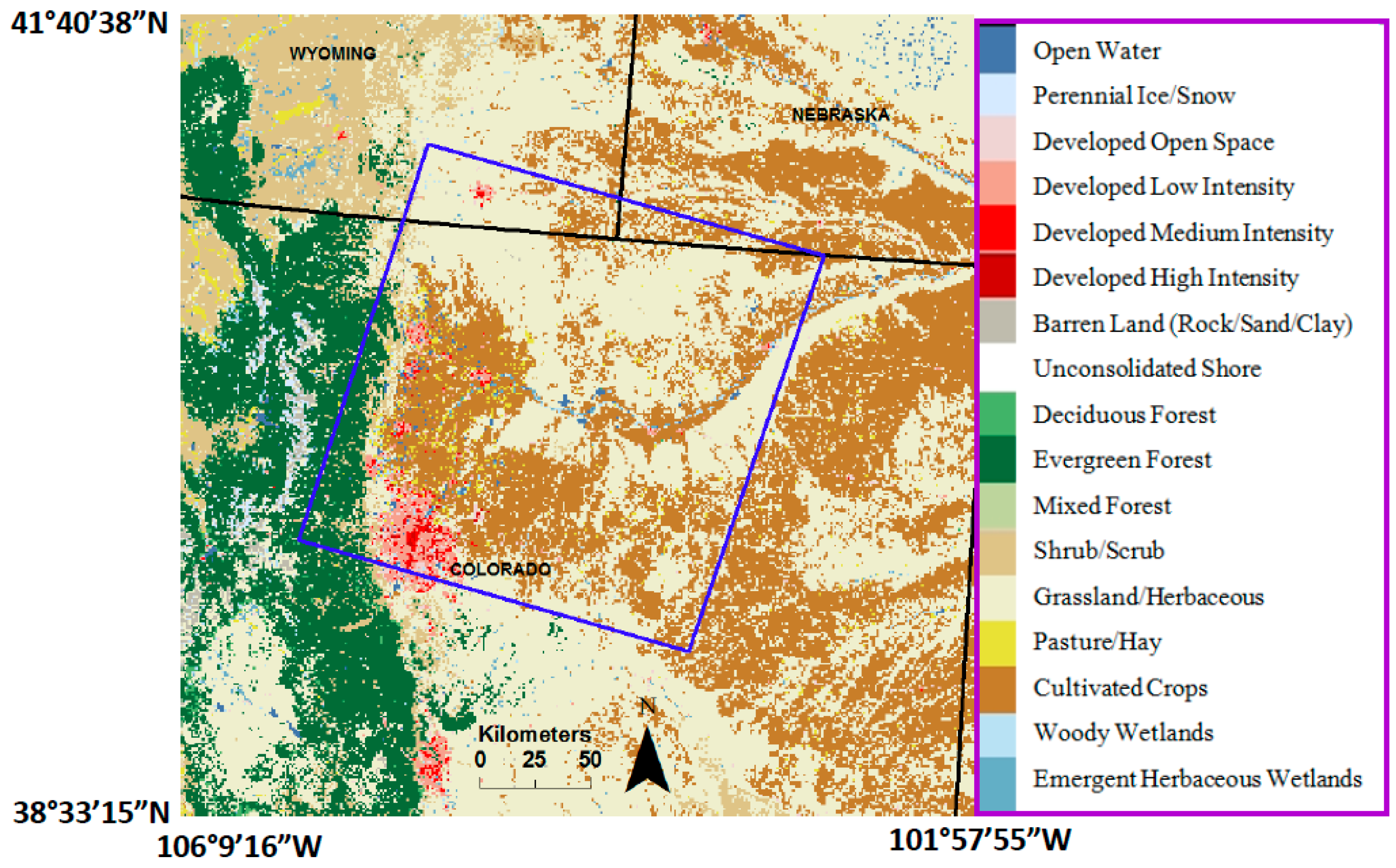
2.1. Study Area

2.2. Data
2.2.1. Landsat Data
2.2.2. MODIS GSN Data
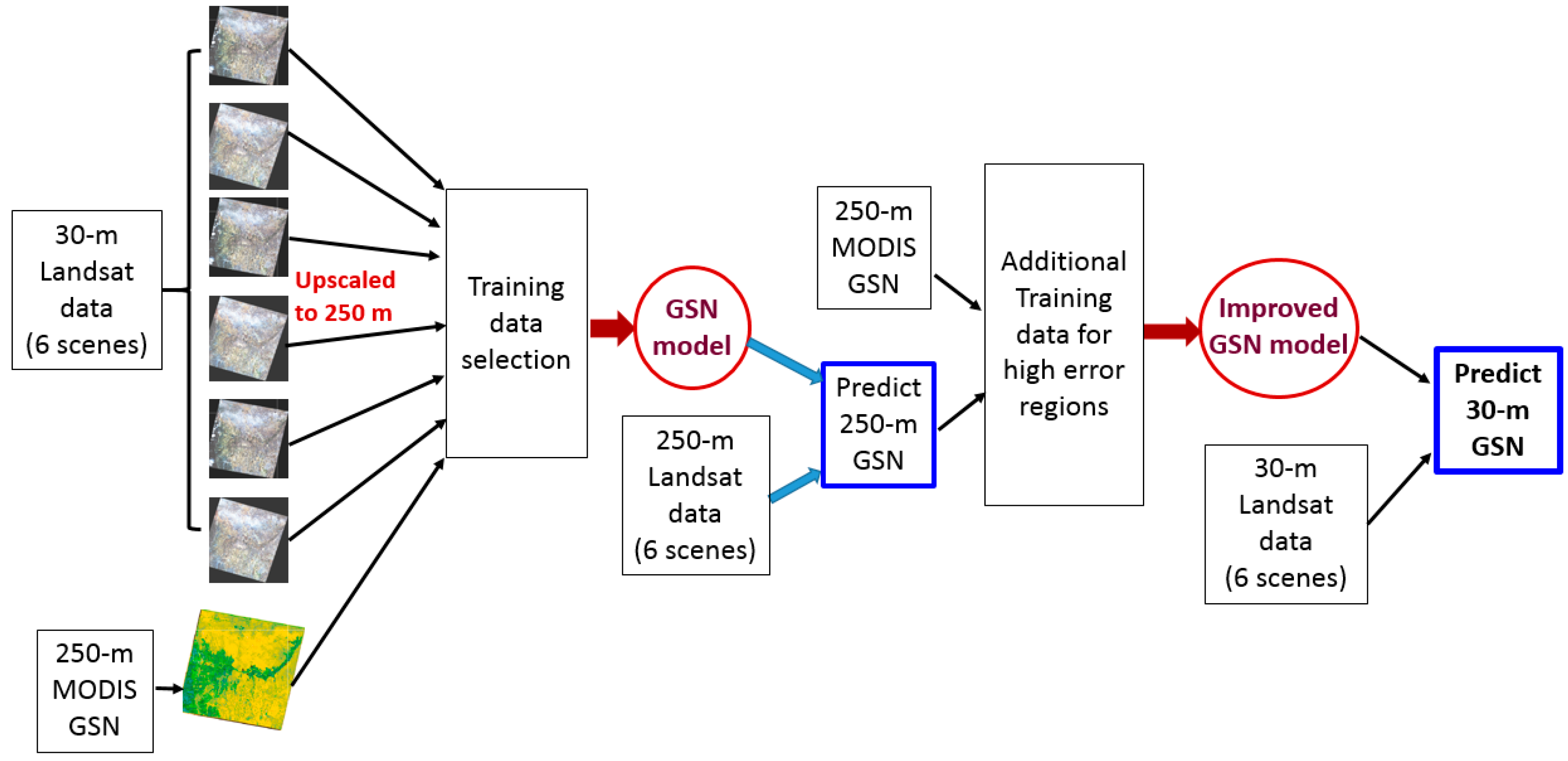
2.3. Approach for Developing a 30-m GSN Map Based on MODIS and Landsat Data
2.3.1. Building Rule-based Piecewise Regression GSN Models
2.3.2. Improving the GSN Model for Developing a 30-m MODIS-Landsat GSN Map

2.3.3. Evaluating the 30-m MODIS-Landsat GSN Map
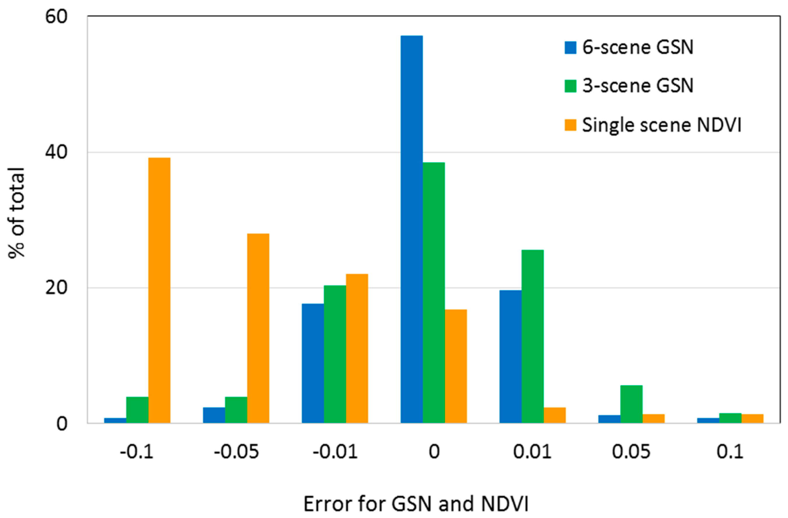
2.4. Testing and Identifying the Optimal Landsat Date Combinations for the GSN Model
3. Results and Discussion
3.1. GSN Regression Tree Model for the Cloud-Free Pixels


| 6-Scene | Highest r for the 5-Scene Combination | Lowest r for the 5-Scene Combination | Highest r for the 3-Scene Combination | Lowest r for the 3-Scene Combination | |
|---|---|---|---|---|---|
| Month | 4–9 | 4,5,6,8,9 | 4,6,7,8,9 | 5,7,9 (or 6,8,9) | 4,5,6 |
| r | 0.98 | 0.98 | 0.97 | 0.98 | 0.93 |
| Average error | 0.015 | 0.014 | 0.015 | 0.015 | 0.026 |

3.2. GSN Regression Tree Model for the “Clear and Cloudy” Pixels
| Name | Usage in Rule Stratification | Usage in Regression Model | Average Usage |
|---|---|---|---|
| 8NDVI | 74% | 81% | 78% |
| 5NDVI | 55% | 81% | 68% |
| 4B5 | 32% | 58% | 45% |
| 4NDVI | 29% | 61% | 45% |
| 9NDVI | 14% | 74% | 44% |
| 6NDVI | 32% | 53% | 43% |
| 9B4 | 19% | 65% | 42% |
| 7NDVI | 11% | 73% | 42% |
| 5B3 | 16% | 67% | 42% |
| 8B1 | 16% | 65% | 41% |
| 5B1 | 8% | 66% | 37% |
| 8B2 | 6% | 68% | 37% |
| 9B3 | 3% | 70% | 37% |
| 8B4 | 7% | 63% | 35% |
| 9B1 | 6% | 64% | 35% |
| 8B3 | 70% | - | 35% |
| 9B2 | 70% | - | 35% |
| 4B2 | 2% | 64% | 33% |
| 5B4 | 8% | 58% | 33% |
| 5B2 | 3% | 62% | 33% |
| 5B5 | 26% | 35% | 31% |
| 4B4 | 6% | 54% | 30% |
| 7B3 | 1% | 59% | 30% |
| 4B1 | 59% | - | 30% |
| 7B2 | 2% | 53% | 28% |
| 6B3 | 2% | 53% | 28% |
| 7B5 | 9% | 45% | 27% |
| 7B4 | 1% | 53% | 27% |
| 4B3 | 53% | - | 27% |
| 9B5 | 2% | 44% | 23% |
| 6B4 | 5% | 40% | 23% |
| 6B2 | 1% | 44% | 23% |
| 8B5 | 42% | - | 21% |
| 6B1 | 2% | 38% | 20% |
| 6B5 | 9% | 30% | 20% |
| 7B1 | 2% | 33% | 18% |
| 6Fmask | 7% | - | 4% |
| Month | 456 | 457 | 458 | 459 | 467 | 468 | 469 | 478 | 479 | 489 |
|---|---|---|---|---|---|---|---|---|---|---|
| Correlation coefficient (r) | 0.95 | 0.95 | 0.95 | 0.93 | 0.93 | 0.94 | 0.94 | 0.94 | 0.94 | 0.93 |
| Absolute average error (×100) | 3.9 | 3.3 | 3.1 | 3.8 | 3.7 | 3.3 | 3.6 | 3.6 | 3.5 | 3.6 |
| Month | 567 | 568 | 569 | 578 | 579 | 589 | 678 | 679 | 689 | 789 |
| Correlation coefficient (r) | 0.96 | 0.96 | 0.96 | 0.95 | 0.95 | 0.96 | 0.94 | 0.93 | 0.95 | 0.91 |
| Absolute average error (×100) | 3.3 | 2.9 | 3.3 | 3.1 | 3.1 | 3.2 | 3.6 | 3.6 | 3.3 | 4.2 |
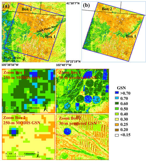
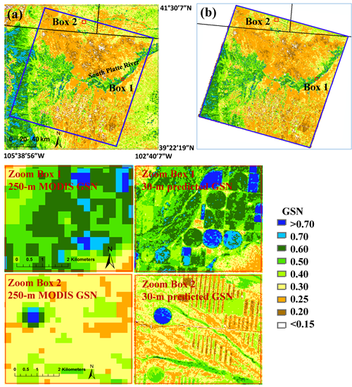
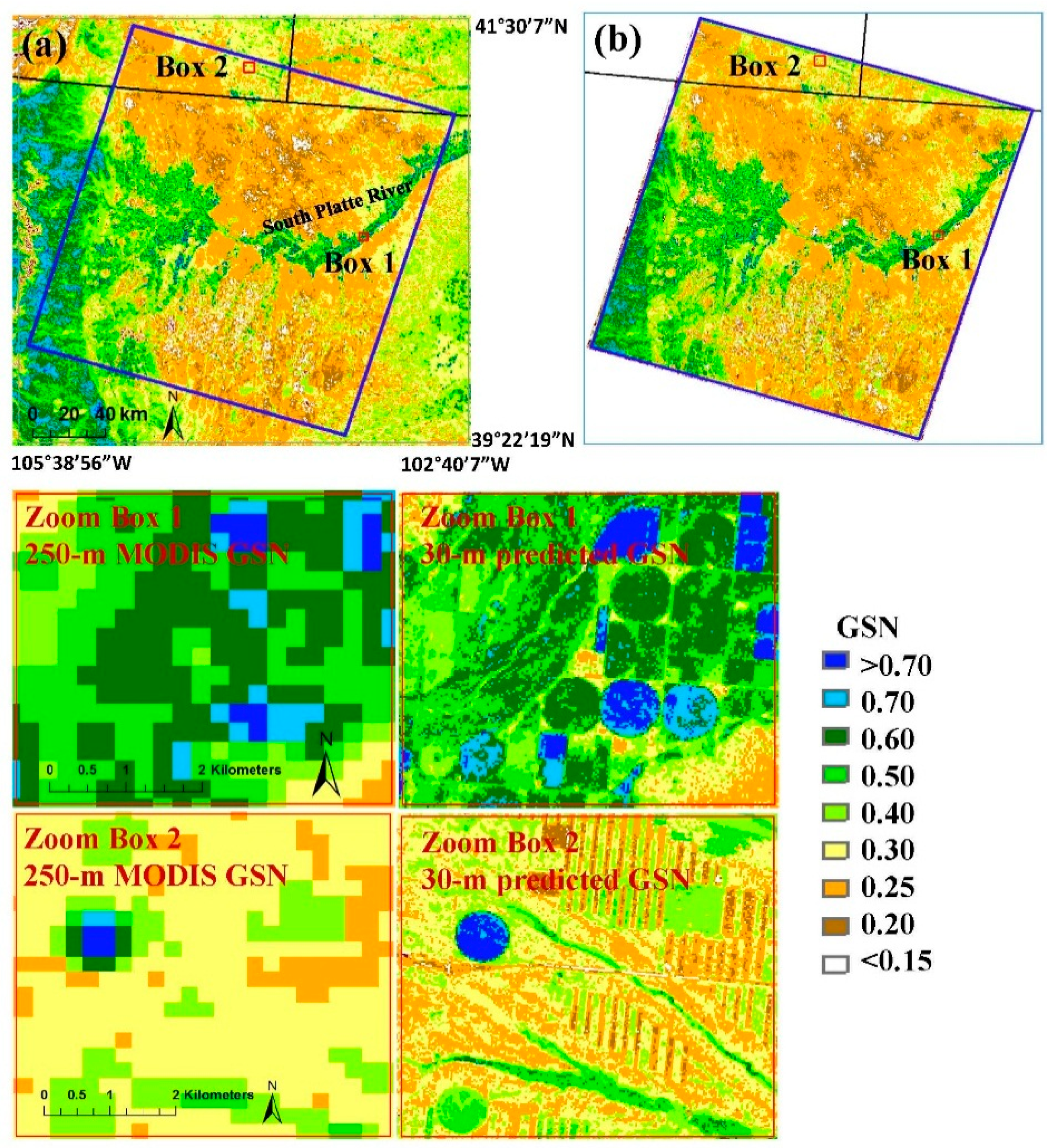
3.3. MODIS-Landsat GSN Map
3.3.1. Comparing the Predicted 30-m GSN with the 250-m MODIS GSN


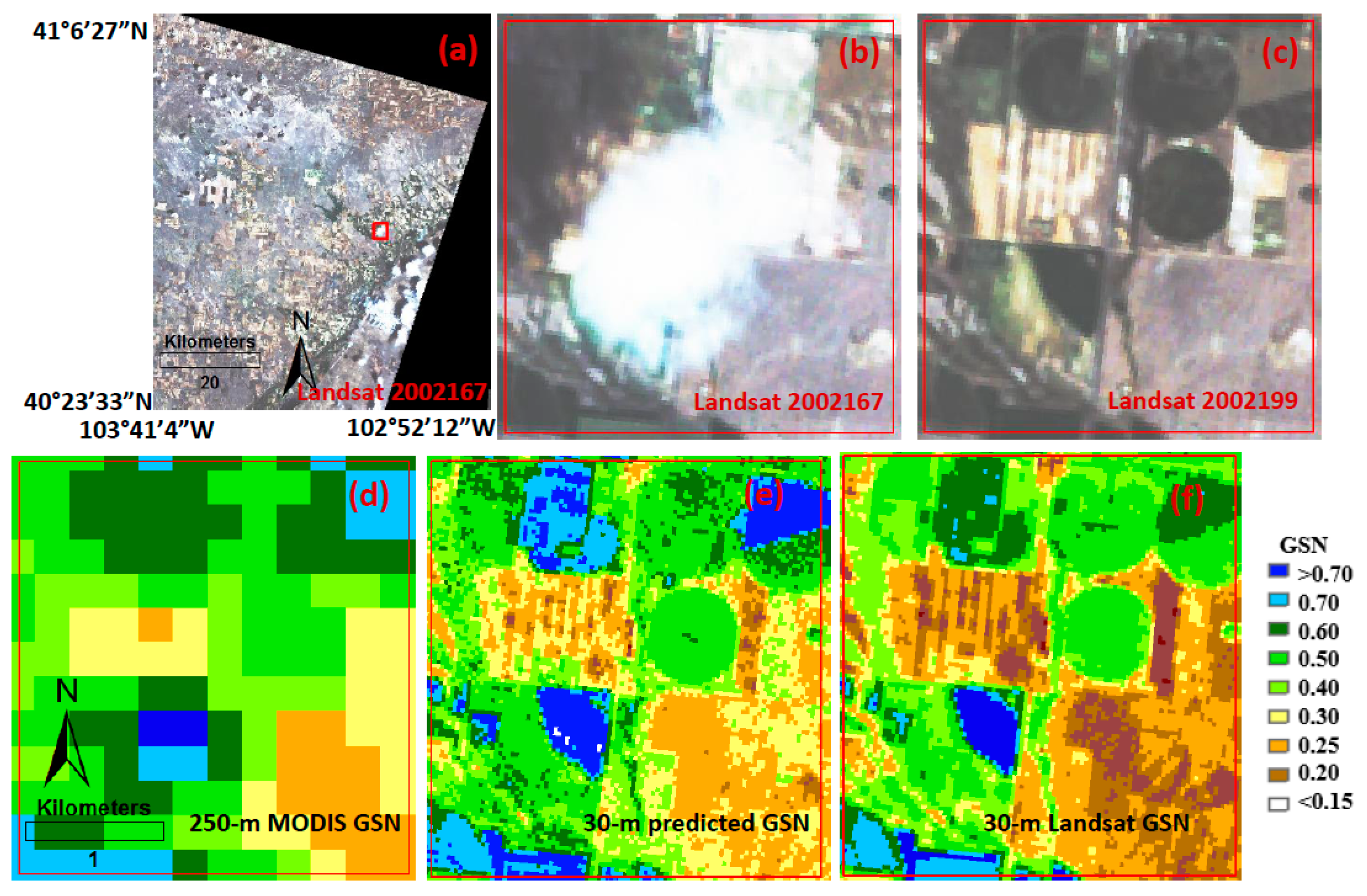
3.3.2. Assessing the Impacts of Clouds
3.4. Discussion
4. Conclusions
Acknowledgments
Author Contributions
Conflicts of Interest
References
- Anderson, J.R.; Hardy, E.E.; Roach, J.T.; Witmer, R.E. A Land Use and Land Cover Classification System for Use with Remote Sensor Data; U.S. Geological Survey: Reston, VA, USA, 1976; p. 28. [Google Scholar]
- Reed, B.C.; Brown, J.F.; Vanderzee, D.; Loveland, T.R.; Merchant, J.W.; Ohlen, D.O. Measuring phenological variability from satellite imagery. J. Veg. Sci. 1994, 5, 703–714. [Google Scholar] [CrossRef]
- Peters, A.J.; Walter-Shea, E.A.; Ji, L.; Viña, A.; Hayes, M.; Svoboda, M.D. Drought monitoring with NDVI-based standardized vegetation index. Photogramm. Eng. Remote Sens. 2002, 68, 71–75. [Google Scholar]
- Gu, Y.; Brown, J.F.; Verdin, J.P.; Wardlow, B. A five-year analysis of MODIS NDVI and NDWI for grassland drought assessment over the central great plains of the United States. Geophys. Res. Lett. 2007, 34. [Google Scholar] [CrossRef]
- Gu, Y.; Wylie, B.K. Detecting ecosystem performance anomalies for land management in the upper Colorado river basin using satellite observations, climate data, and ecosystem models. Remote Sens. 2010, 2, 1880–1891. [Google Scholar] [CrossRef]
- Wylie, B.K.; Zhang, L.; Bliss, N.B.; Ji, L.; Tieszen, L.L.; Jolly, W.M. Integrating modelling and remote sensing to identify ecosystem performance anomalies in the boreal forest, Yukon river basin, Alaska. Int. J. Digit. Earth 2008, 1, 196–220. [Google Scholar] [CrossRef]
- Gu, Y.; Boyte, S.P.; Wylie, B.K.; Tieszen, L.L. Identifying grasslands suitable for cellulosic feedstock crops in the greater Platte river basin: Dynamic modeling of ecosystem performance with 250 m eMODIS. GCB Bioenergy 2012, 4, 96–106. [Google Scholar] [CrossRef]
- Kimball, J.S.; Zhao, M.; McDonald, K.C.; Running, S.W. Satellite remote sensing of terrestrial net primary production for the pan-Arctic basin and Alaska. Mitig. Adapt. Strateg. Glob. Chang. 2006, 11, 783–804. [Google Scholar] [CrossRef]
- Rouse, J.W., Jr.; Haas, H.R.; Deering, D.W.; Schell, J.A.; Harlan, J.C. Monitoring the Vernal Advancement and Retrogradation (Green Wave Effect) of Natural Vegetation; Texas A and M University: Greenbelt, MD, USA, 1974. [Google Scholar]
- Tucker, C.J. Red and photographic infrared linear combinations for monitoring vegetation. Remote Sens. Environ. 1979, 8, 127–150. [Google Scholar] [CrossRef]
- Chen, D.; Brutsaert, W. Satellite-sensed distribution and spatial patterns of vegetation parameters over a tallgrass prairie. J. Atmos. Sci. 1998, 55, 1225–1238. [Google Scholar] [CrossRef]
- Ollinger, S.V. Sources of variability in canopy reflectance and the convergent properties of plants. New Phytol. 2011, 189, 375–394. [Google Scholar] [CrossRef] [PubMed]
- Tucker, C.J.; Vanpraet, C.L.; Sharman, M.J.; van Ittersum, G. Satellite remote sensing of total herbaceous biomass production in the Senegalese Sahel: 1980–1984. Remote Sens. Environ. 1985, 17, 233–249. [Google Scholar] [CrossRef]
- Hobbs, T.J. The use of NOAA-AVHRR NDVI data to assess herbage production in the arid rangelands of Central Australia. Int. J. Remote Sens. 1995, 16, 1289–1302. [Google Scholar] [CrossRef]
- Tieszen, L.L.; Reed, B.C.; Bliss, N.B.; Wylie, B.K.; DeJong, D.D. NDVI, C3 and C4 production, and distributions in Great Plains grassland land cover classes. Ecol. Appl. 1997, 7, 59–78. [Google Scholar]
- Gitelson, A.A.; Viña, A.; Verma, S.B.; Rundquist, D.C.; Arkebauer, T.J.; Keydan, G.; Leavitt, B.; Ciganda, V.; Burba, G.G.; Suyker, A.E. Relationship between gross primary production and chlorophyll content in crops: Implications for the synoptic monitoring of vegetation productivity. J. Geophys. Res. Atmos. 2006, 111. [Google Scholar] [CrossRef]
- Funk, C.; Budde, M.E. Phenologically-tuned MODIS NDVI-based production anomaly estimates for Zimbabwe. Remote Sens. Environ. 2009, 113, 115–125. [Google Scholar] [CrossRef]
- Becker-Reshef, I.; Vermote, E.; Lindeman, M.; Justice, C. A generalized regression-based model for forecasting winter wheat yields in Kansas and Ukraine using MODIS data. Remote Sens. Environ. 2010, 114, 1312–1323. [Google Scholar] [CrossRef]
- Gu, Y.; Wylie, B.K.; Bliss, N.B. Mapping grassland productivity with 250-m eMODIS NDVI and SSURGO database over the greater Platte river basin, USA. Ecol. Indic. 2013, 24, 31–36. [Google Scholar] [CrossRef]
- Wylie, B.K.; Denda, I.; Pieper, R.D.; Harrington, J.A.; Reed, B.C.; Southward, G.M. Satellite-based herbaceous biomass estimates in the pastoral zone of Niger. J. Range Manag. 1995, 48, 159–164. [Google Scholar] [CrossRef]
- Hatfield, J.L.; Kanemasu, E.T.; Asrar, G.; Jackson, R.D.; Pinter, P.J.; Reginato, R.J.; Idso, S.B. Leaf-area estimates from spectral measurements over various planting dates of wheat. Int. J. Remote Sens. 1985, 6, 167–175. [Google Scholar] [CrossRef]
- Asrar, G.; Fuchs, M.; Kanemasu, E.T.; Hatfield, J.L. Estimating absorbed photosynthetic radiation and leaf area index from spectral reflectance in wheat. Agron. J. 1984, 76, 300–306. [Google Scholar] [CrossRef]
- Chen, P.-Y.; Fedosejevs, G.; Tiscareño-López, M.; Arnold, J.G. Assessment of MODIS-EVI, MODIS-NDVI and vegetation-NDVI composite data using agricultural measurements: An example at corn fields in Western Mexico. Environ. Monit. Assess. 2006, 119, 69–82. [Google Scholar] [CrossRef] [PubMed]
- Asner, G.P.; Scurlock, J.M.O.; Hicke, J.A. Global synthesis of leaf area index observations: Implications for ecological and remote sensing studies. Glob. Ecol. Biogeogr. 2003, 12, 191–205. [Google Scholar] [CrossRef]
- Sellers, P.J. Canopy reflectance, photosynthesis and transpiration. Int. J. Remote Sens. 1985, 6, 1335–1372. [Google Scholar] [CrossRef]
- Gu, Y.; Wylie, B.K.; Howard, D.M.; Phuyal, K.P.; Ji, L. NDVI saturation adjustment: A new approach for improving cropland performance estimates in the greater Platte river basin, USA. Ecol. Indic. 2013, 30, 1–6. [Google Scholar] [CrossRef]
- Potter, C.; Klooster, S.; Huete, A.; Genovese, V. Terrestrial carbon sinks for the United States predicted from MODIS satellite data and ecosystem modeling. Earth Interact. 2007, 11, 1–21. [Google Scholar] [CrossRef]
- NASA MODIS Web. Available online: http://modis.gsfc.nasa.gov/ (accessed on 22 January 2015).
- Land Processes Distributed Active Archive Center. Available online: https://lpdaac.usgs.gov/products/modis_products_table/modis_overview (accessed on March 20 2015).
- Wylie, B.K.; Boyte, S.P.; Major, D.J. Ecosystem performance monitoring of rangelands by integrating modeling and remote sensing. Rangel. Ecol. Manag. 2012, 65, 241–252. [Google Scholar] [CrossRef]
- Rigge, M.; Smart, A.; Wylie, B.; Gilmanov, T.; Johnson, P. Linking phenology and biomass productivity in South Dakota mixed-grass prairie. Rangel. Ecol. Manag. 2013, 66, 579–587. [Google Scholar] [CrossRef]
- Tan, Z.; Liu, S.; Wylie, B.K.; Jenkerson, C.B.; Oeding, J.; Rover, J.; Young, C. MODIS-informed greenness responses to daytime land surface temperature fluctuations and wildfire disturbances in the Alaskan Yukon river basin. Int. J. Remote Sens. 2012, 34, 2187–2199. [Google Scholar] [CrossRef]
- Spruce, J.P.; Sader, S.; Ryan, R.E.; Smoot, J.; Kuper, P.; Ross, K.; Prados, D.; Russell, J.; Gasser, G.; McKellip, R.; et al. Assessment of MODIS NDVI time series data products for detecting forest defoliation by gypsy moth outbreaks. Remote Sens. Environ. 2011, 115, 427–437. [Google Scholar] [CrossRef]
- NASA Landsat Science. Available online: http://landsat.gsfc.nasa.gov/ (accessed on 22 January 2015).
- Williams, D.L.; Goward, S.; Arvldson, T. Landsat: Yesterday, today, and tomorrow. Photogramm. Eng. Remote Sens. 2006, 72, 1171–1178. [Google Scholar] [CrossRef]
- Goward, S.N.; Masek, J.G.; Williams, D.L.; Irons, J.R.; Thompson, R.J. The Landsat 7 mission—Terrestrial research and applications for the 21st century. Remote Sens. Environ. 2001, 78, 3–12. [Google Scholar] [CrossRef]
- Homer, C.; Huang, C.; Yang, L.; Wylie, B.; Coan, M. Development of a 2001 national land-cover database for the United States. Photogramm. Eng. Remote Sens. 2004, 70, 829–840. [Google Scholar] [CrossRef]
- Wulder, M.A.; White, J.C.; Goward, S.N.; Masek, J.G.; Irons, J.R.; Herold, M.; Cohen, W.B.; Loveland, T.R.; Woodcock, C.E. Landsat continuity: Issues and opportunities for land cover monitoring. Remote Sens. Environ. 2008, 112, 955–969. [Google Scholar] [CrossRef]
- Goward, S.N.; Williams, D.L. Landsat and earth systems science: Development of terrestrial monitoring. Photogramm. Eng. Remote Sens. 1997, 63, 887–900. [Google Scholar]
- Huang, C.; Goward, S.; Masek, J.; Thomas, N.; Zhu, Z.; Vogelmann, J. An automated approach for reconstructing recent forest disturbance history using dense Landsat time series stacks. Remote Sens. Environ. 2010, 114, 183–198. [Google Scholar] [CrossRef]
- Huang, C.; Kim, S.; Song, K.; Townshend, J.R.G.; Davis, P.; Altstatt, A.; Rodas, O.; Yanosky, A.; Clay, R.; Tucker, C.J.; et al. Assessment of Paraguay’s forest cover change using Landsat observations. Glob. Planet. Change 2009, 67, 1–12. [Google Scholar] [CrossRef]
- Vogelmann, J.E.; Xian, G.; Homer, C.; Tolk, B. Monitoring gradual ecosystem change using Landsat time series analyses: Case studies in selected forest and rangeland ecosystems. Remote Sens. Environ. 2012, 122, 92–105. [Google Scholar] [CrossRef]
- Gasparri, N.I.; Parmuchi, M.G.; Bono, J.; Karszenbaum, H.; Montenegro, C.L. Assessing multi-temporal Landsat 7 ETM+ images for estimating above-ground biomass in subtropical dry forests of Argentina. J. Arid Environ. 2010, 74, 1262–1270. [Google Scholar] [CrossRef]
- Röder, A.; Udelhoven, T.; Hill, J.; del Barrio, G.; Tsiourlis, G. Trend analysis of Landsat-TM and -ETM+ imagery to monitor grazing impact in a rangeland ecosystem in Northern Greece. Remote Sens. Environ. 2008, 112, 2863–2875. [Google Scholar] [CrossRef]
- Xian, G.; Crane, M. An analysis of urban thermal characteristics and associated land cover in Tampa bay and Las Vegas using Landsat satellite data. Remote Sens. Environ. 2006, 104, 147–156. [Google Scholar] [CrossRef]
- Herold, N.D.; Haack, B.N. Comparison and integration of radar and optical data for land use/cover mapping. Geocarto Int. 2006, 21, 9–19. [Google Scholar] [CrossRef]
- Spruce, J.P.; Smoot, J.C.; Ellis, J.T.; Hilbert, K.; Swann, R. Geospatial method for computing supplemental multi-decadal us coastal land use and land cover classification products, using Landsat data and C-CAP products. Geocarto Int. 2014, 29, 470–485. [Google Scholar] [CrossRef]
- Spruce, J.P.; Smoot, J.; Graham, W. Developing new coastal forest restoration products based on Landsat, Aster, and MODIS data. In Proceedings of the MTS/IEEE Biloxi—Marine Technology for Our Future: Global and Local Challenges, OCEANS 2009, Biloxi, MS, USA, 26–29 October 2009.
- USGS Landsat Missions. Available online: http://landsat.usgs.gov/ (accessed on 22 January 2015).
- Gao, F.; Masek, J.; Schwaller, M.; Hall, F. On the blending of the Landsat and MODIS surface reflectance: Predicting daily Landsat surface reflectance. IEEE Trans. Geosci. Remote Sens. 2006, 44, 2207–2218. [Google Scholar] [CrossRef]
- Irish, R.R.; Barker, J.L.; Goward, S.N.; Arvidson, T. Characterization of the landsat-7 ETM+ automated cloud-cover assessment (ACCA) algorithm. Photogramm. Eng. Remote Sens. 2006, 72, 1179–1188. [Google Scholar] [CrossRef]
- Ju, J.; Roy, D.P. The availability of cloud-free Landsat ETM+ data over the conterminous United States and globally. Remote Sens. Environ. 2008, 112, 1196–1211. [Google Scholar] [CrossRef]
- Roy, D.P.; Ju, J.; Lewis, P.; Schaaf, C.; Gao, F.; Hansen, M.; Lindquist, E. Multi-temporal MODIS-Landsat data fusion for relative radiometric normalization, gap filling, and prediction of Landsat data. Remote Sens. Environ. 2008, 112, 3112–3130. [Google Scholar] [CrossRef]
- Ackerman, S.A.; Strabala, K.I.; Menzel, W.P.; Frey, R.A.; Moeller, C.C.; Gumley, L.E. Discriminating clear sky from clouds with MODIS. J. Geophys. Res. Atmos. 1998, 103, 32141–32157. [Google Scholar] [CrossRef]
- Platnick, S.; King, M.D.; Ackerman, S.A.; Menzel, W.P.; Baum, B.A.; Riédi, J.C.; Frey, R.A. The MODIS cloud products: Algorithms and examples from terra. IEEE Trans. Geosci. Remote Sens. 2003, 41, 459–472. [Google Scholar] [CrossRef]
- Helmer, E.H.; Ruefenacht, B. Cloud-free satellite image mosaics with regression trees and histogram matching. Photogramm. Eng. Remote Sens. 2005, 71, 1079–1089. [Google Scholar] [CrossRef]
- Kaufman, Y.J.; Wald, A.E.; Remer, L.A.; Gao, B.-C.; Li, R.-R.; Flynn, L. MODIS 2.1-μm channel—Correlation with visible reflectance for use in remote sensing of aerosol. IEEE Trans. Geosci. Remote Sens. 1997, 35, 1286–1298. [Google Scholar] [CrossRef]
- USGS Global Visualization Viewer. Available online: http://glovis.usgs.gov/ (accessed on 22 January 2015).
- USGS CDR Data. Available online: http://landsat.usgs.gov/CDR_LSR.php (accessed on 22 January 2015).
- NASA LEDAPS. Available online: http://ledapsweb.nascom.nasa.gov/ (accessed on 22 January 2015).
- Jenkerson, C.B.; Maiersperger, T.K.; Schmidt, G.L. eMODIS—A User-Friendly Data Source. Available online: http://pubs.usgs.gov/of/2010/1055/ (accessed on 22 January 2015).
- Swets, D.L.; Reed, B.C.; Rowland, J.R.; Marko, S.E. A weighted least-squares approach to temporal smoothing of NDVI. In Proceedings of the ASPRS Annual Conference, from Image to Information, Portland, OR, USA, 17–21 May1999.
- USGS Remote Sensing Phenology. Available online: http://phenology.cr.usgs.gov/ (accessed on 22 January 2015).
- RuleQuest Research. Available online: http://www.rulequest.com/ (accessed on March 20 2015).
- Gu, Y.; Howard, D.; Wylie, B.; Zhang, L. Mapping carbon flux uncertainty and selecting optimal locations for future flux towers in the Great Plains. Landsc. Ecol. 2012, 27, 319–326. [Google Scholar] [CrossRef]
- Zhang, L.; Wylie, B.K.; Ji, L.; Gilmanov, T.G.; Tieszen, L.L. Climate-driven interannual variability in net ecosystem exchange in the Northern Great Plains grasslands. Rangel. Ecol. Manag. 2010, 63, 40–50. [Google Scholar] [CrossRef]
- Boyte, S.P.; Wylie, B.K.; Major, D.J.; Brown, J.F. The integration of geophysical and enhanced moderate resolution imaging spectroradiometer normalized difference vegetation index data into a rule-based, piecewise regression-tree model to estimate cheatgrass beginning of spring growth. Int. J. Digit. Earth 2013, 8, 1–15. [Google Scholar]
- Ji, L.; Wylie, B.K.; Nossov, D.R.; Peterson, B.E.; Waldrop, M.P.; McFarland, J.W.; Rover, J.A.; Hollingsworth, T.N. Estimating aboveground biomass in interior Alaska with Landsat data and field measurements. Int. J. Appl. Earth Obs. Geoinf. 2012, 18, 451–461. [Google Scholar] [CrossRef]
- Rover, J.; Wylie, B.K.; Ji, L. A self-trained classification technique for producing 30 m percent-water maps from Landsat data. Int. J. Remote Sens. 2010, 31, 2197–2203. [Google Scholar] [CrossRef]
- Quinlan, J.R. Boosting first-order learning. In Algorithmic Learning Theory; Arikawa, S., Sharma, A., Eds.; Springer Berlin Heidelberg: Berlin, Germany, 1996; Volume 1160, pp. 143–155. [Google Scholar]
- Trishchenko, A.P.; Luo, Y.; Khlopenkov, K.V. A method for downscaling MODIS land channels to 250-m spatial resolution using adaptive regression and normalization. Proc. SPIE 2006, 6366. [Google Scholar] [CrossRef]
- Hwang, T.; Song, C.; Bolstad, P.V.; Band, L.E. Downscaling real-time vegetation dynamics by fusing multi-temporal MODIS and Landsat NDVI in topographically complex terrain. Remote Sens. Environ. 2011, 115, 2499–2512. [Google Scholar] [CrossRef]
- Bindhu, V.M.; Narasimhan, B.; Sudheer, K.P. Development and verification of a non-linear disaggregation method (NL-DisTrad) to downscale MODIS land surface temperature to the spatial scale of Landsat thermal data to estimate evapotranspiration. Remote Sens. Environ. 2013, 135, 118–129. [Google Scholar] [CrossRef]
- Atkinson, P.M. Downscaling in remote sensing. Int. J. Appl. Earth Obs. Geoinf. 2013, 22, 106–114. [Google Scholar] [CrossRef]
- Hansen, M.C.; Roy, D.P.; Lindquist, E.; Adusei, B.; Justice, C.O.; Altstatt, A. A method for integrating MODIS and Landsat data for systematic monitoring of forest cover and change in the Congo basin. Remote Sens. Environ. 2008, 112, 2495–2513. [Google Scholar] [CrossRef]
- Hong, S.-H.; Hendrickx, J.M.H.; Borchers, B. Down-scaling of SEBAL derived evapotranspiration maps from MODIS (250 m) to Landsat (30 m) scales. Int. J. Remote Sens. 2011, 32, 6457–6477. [Google Scholar] [CrossRef]
- Kim, J.; Hogue, T.S. Evaluation and sensitivity testing of a coupled Landsat-MODIS downscaling method for land surface temperature and vegetation indices in semi-arid regions. J. Appl. Remote Sens. 2012, 6. [Google Scholar] [CrossRef]
- Zhu, Z.; Woodcock, C.E. Continuous change detection and classification of land cover using all available Landsat data. Remote Sens. Environ. 2014, 144, 152–171. [Google Scholar] [CrossRef]
© 2015 by the authors; licensee MDPI, Basel, Switzerland. This article is an open access article distributed under the terms and conditions of the Creative Commons Attribution license (http://creativecommons.org/licenses/by/4.0/).
Share and Cite
Gu, Y.; Wylie, B.K. Downscaling 250-m MODIS Growing Season NDVI Based on Multiple-Date Landsat Images and Data Mining Approaches. Remote Sens. 2015, 7, 3489-3506. https://doi.org/10.3390/rs70403489
Gu Y, Wylie BK. Downscaling 250-m MODIS Growing Season NDVI Based on Multiple-Date Landsat Images and Data Mining Approaches. Remote Sensing. 2015; 7(4):3489-3506. https://doi.org/10.3390/rs70403489
Chicago/Turabian StyleGu, Yingxin, and Bruce K. Wylie. 2015. "Downscaling 250-m MODIS Growing Season NDVI Based on Multiple-Date Landsat Images and Data Mining Approaches" Remote Sensing 7, no. 4: 3489-3506. https://doi.org/10.3390/rs70403489