1. Introduction
Recognizing a need for nationally comprehensive and consistent geospatial data describing wildfire fuels and fire regimes, the Landscape Fire and Resource Management Planning Tools (LANDFIRE) program was chartered in 2004 as a joint effort between the US Department of Agriculture and the US Department of the Interior [
1]. LANDFIRE has produced maps of vegetation and fuels for the entire US, at 30 m resolution, which are used for both tactical and strategic decision-making by incident commanders and land managers, along with many other ecological research applications [
2].
Currently there exist various versions of LANDFIRE data products for all of the conterminous US (CONUS), Hawai’i, and Alaska (see [
3] for more information regarding the LANDFIRE product versions). The first LANDFIRE National data products in Alaska were released in 2009, including maps of existing canopy height. The LANDFIRE mapping methods typically make use of available field observations to inform the mapping process. Various field datasets contributed by federal and state agencies, universities and other programs have been incorporated into the LANDFIRE reference database. For example, data from the US Forest Service’s Forest Inventory and Analysis (FIA) program are relied on for different aspects of forest mapping. The FIA data are consistently high quality and provide information about vegetation composition and structure [
4]. In Alaska, FIA data are available only for the southeastern part of the state, leaving vast portions of the state, especially the boreal forests of interior Alaska, un-inventoried. Furthermore, field observations from other sources in Alaska are also sparse or lack the type of information required by the LANDFIRE mapping methods to be useful.
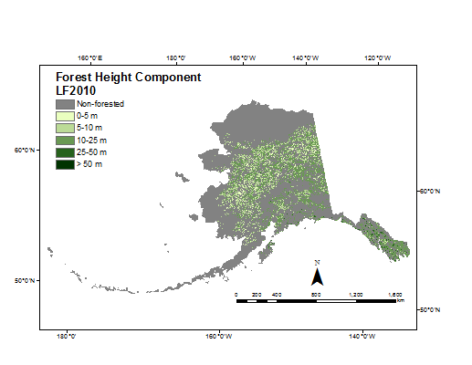
The lack of abundant, high-quality field data affected the mapping strategies used in Alaska and led to modifications of the forest canopy height legend used in the LANDFIRE National existing vegetation height (EVH) product for Alaska. EVH is a composite of forest, shrub, and herbaceous height maps based on the dominant lifeform of the existing vegetation type (EVT) product for each 30 m pixel. Specifically, it was necessary to reduce the number of mapped canopy height classes to reflect the limitations imposed by the paucity of training data. While the standard LANDFIRE forest canopy height product consists of five height classes (0–5 m, 5–10 m, 10–25 m, 25–50 m, and >50 m), in Alaska the same map represented only two classes (≤ 10 m and > 10 m,
Figure 1).
Collecting field data in Alaska is expensive and time consuming because of the remoteness of much of the area. Therefore, exploring the utility of remote sensing data for structure mapping in Alaska is particularly intriguing for assessing Alaskan forest structure. The total area of Alaska is just under 1,700,000 km
2, of which approximately 380,000 km
2, or 22%, is forested, according to the 2001 National Land Cover Dataset (NLCD) [
5]. LiDAR is especially suited for deriving forest canopy structure because of its ability to capture vertical information about the canopy. Airborne LiDAR data have been collected in several locations in Alaska and have been used for measuring aspects of canopy structure. These include studies focused on forest stand condition characterization in the Kenai Peninsula [
6], biomass assessment in the Upper Tanana Valley near Tok [
7], forest canopy height and fuels estimation in the Yukon Flats Ecoregion [
8,
9], and biomass change in the Yukon River Basin [
10].
While these airborne data sets provide detailed information for local areas, vast areas of Alaska remain unmapped by airborne LiDAR systems. To obtain LiDAR observations of structure, the LANDFIRE team decided to explore the use of spaceborne LiDAR data from the ICESat Geoscience Laser Altimeter System (GLAS). GLAS was a large-footprint, waveform-digitizing LiDAR system. GLAS footprint size is nominally 60 m, although this can vary substantially for different laser campaigns, and footprints are spaced 172 m apart, center-to-center, along orbital tracks [
11]. GLAS data represent samples rather than a spatially continuous data layer, and have been used to map various canopy structure elements including height [
12,
13], biomass [
12,
14], and wildfire fuels [
9].
Several limitations on the use of GLAS data for canopy structure exist. One major limitation is the error that can be introduced by high-relief topography. Steep slopes can impact height retrieval from GLAS data by elongating the waveform. Several methods have been proposed for correcting this issue such as demonstrated in [
15,
16].
The classification of the forest height component (FHC) of the LANDFIRE National EVH product in Alaska imposed limits on other products that draw upon the height map and other applications of the data. Therefore, investing effort into an improved Alaska FHC was identified as a priority to better reflect actual landscape conditions. To maintain currency and account for changes within ecosystems, the LANDFIRE products are periodically updated, and as part of the 2010 update to LANDFIRE (LF2010) it was decided to include a remapping of forest height in Alaska using GLAS data [
9]. In [
9], GLAS data are used with airborne LiDAR and Landsat TM imagery to develop canopy height, canopy cover, canopy base height and canopy bulk density layers for the Yukon Flats Ecoregion Alaska. Here, while focused solely on mapping the forest height component (FHC), the incorporation of GLAS data is extended to the entire state of Alaska. The resulting product maps forest canopy height in Alaska using the five height classes defined for CONUS by utilizing available GLAS data with other data sources and represents an improvement over the initial Alaska EVH map released in 2009.
2. Methods
The Alaska FHC remapping effort focused on all lands in Alaska classified as forest in the LANDFIRE EVT map. These lands encompassed a range of forest types, including the tall, dense canopies of the temperate rainforests located in the southeastern part of the state and the open-canopy, short-stature forests more characteristic of the boreal interior.
2.1. Data
Datasets including GLAS waveform LiDAR data, an airborne LiDAR data collection, Landsat imagery, elevation data from the National Elevation Dataset (NED) and associated derivatives (including slope), the 2001 NLCD land cover product, and field data collections were used to accomplish the objectives of this study. These data were used to develop a terrain correction model, build regression tree models to generate geospatial layers of forest height, and to conduct an accuracy assessment of the final map of FHC.
2.1.1. ICEsat GLAS
GLAS version 33 GLA01 and GLA14 products were downloaded from the National Snow and Ice Data Center [
17]. The GLA01 product provides the waveforms while the GLA14 product delivers the footprint coordinates and numerous waveform metrics, including information about the background noise and a set of up to six Gaussian curves fit to the GLAS waveform. Data encompassing the whole GLAS archive including lasers 2 and 3 were downloaded. The data used in this study span the 2003–2009 timeframe. In total there were approximately 5.5 million GLAS footprints located within Alaska for this timeframe, of which over a million are located in forested lands (
Figure 2).
Figure 1.
Original map of LANDFIRE National forest height component for Alaska mapped as two classes.
Figure 1.
Original map of LANDFIRE National forest height component for Alaska mapped as two classes.
2.1.2. Kenai Airborne LiDAR
LiDAR data from an airborne laser scanner (ALS) for the Kenai Peninsula were used to derive the terrain correction coefficients used to address slope-induced error (see
section 2.2.2 below). These data were collected in 2008 during leaf-on conditions and covered approximately 11,750 km
2 of the Kenai Peninsula (
Figure 2) including forested areas with high relief. The nominal point spacing was 2.7 m and the reported horizontal accuracy was 1.3 m. The specifications of the data collection are listed in
Table 1.
Table 1.
Specifications of Kenai airborne LiDAR data acquisition.
Table 1.
Specifications of Kenai airborne LiDAR data acquisition.
| LiDAR System | Optech ALTM Gemini |
|---|
| Ground Speed | 180 kts |
| Pulse Rate Frequency | 33 kHz |
| Mirror Scan Frequency | 17 Hz |
| Scan Angle (+/−) | 15° |
| Beam Divergence | Narrow (0.25 rad) |
| Scan Cutoff | 0.25° |
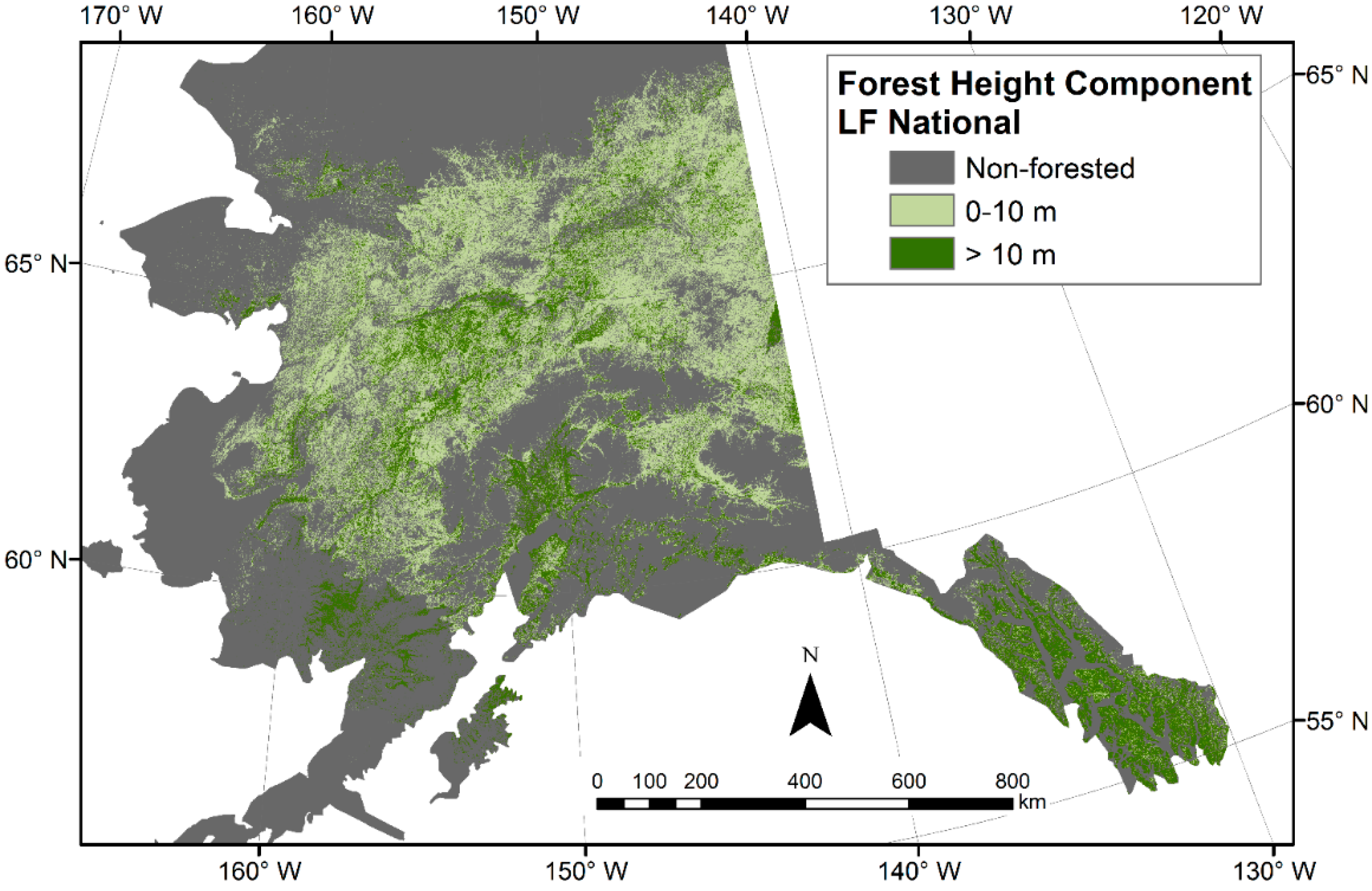
Figure 2.
Map of Alaska showing the distribution of the GLAS spaceborne LiDAR, airborne LiDAR collected over the Kenai Peninsula, and various field observations used for the accuracy assessment of the final forest canopy height product.
Figure 2.
Map of Alaska showing the distribution of the GLAS spaceborne LiDAR, airborne LiDAR collected over the Kenai Peninsula, and various field observations used for the accuracy assessment of the final forest canopy height product.
2.1.3. Landsat Imagery
Landsat imagery were obtained from the Web-Enabled Landsat Data (WELD) project [
18]. WELD provides seasonal and annual composites for the CONUS and Alaska built from Landsat 7 ETM+ imagery. The ETM+ scan-line corrector (SLC) failed in 2003 leaving gaps along the edges of each scene, rendering approximately 22% of each scene as missing data [
19]. The WELD composites effectively fill these gaps with imagery from overlapping paths and other acquisition dates, though often some artifacts remain in the gap areas caused by differences in phenology, illumination, landscape disturbance,
etc. between the various scenes used to create the composite. To minimize the artifacts in the WELD data, annual composites were acquired for each year between 2003 and 2012. These layers were then combined into a “super-composite” by selecting the pixel with the maximum Normalized Difference Vegetation Index value from among the available images at each pixel location [
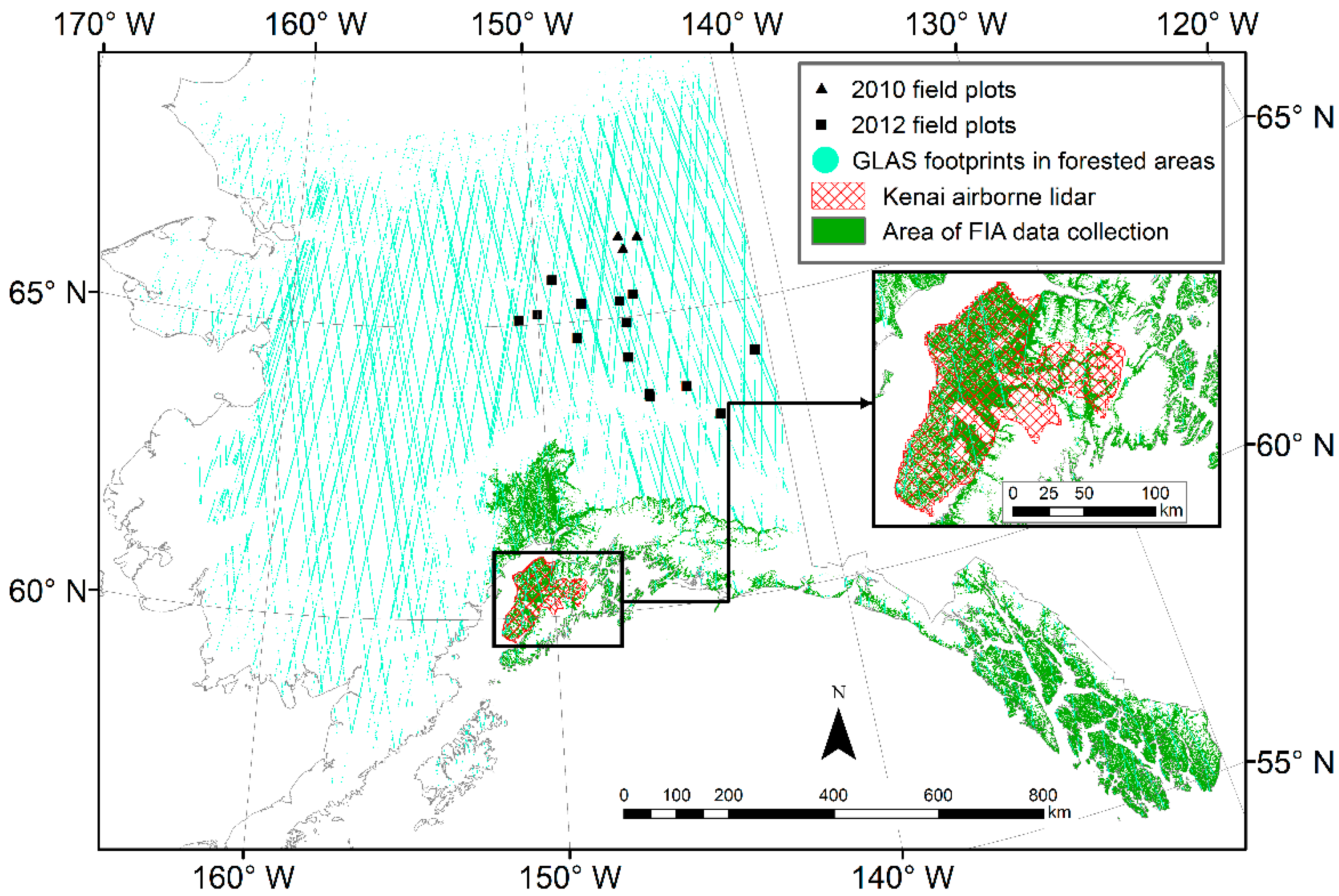
20]. The resultant combination of ten years of imagery provided a statewide composite with noticeably fewer SLC-related artifacts, though some still were apparent, mostly in the southeastern portion of the state (
Figure 3).
2.1.4. Field Data
Field sampled data from three different programs were used to conduct an accuracy assessment of the final FHC map (
Figure 2). First, data from 1106 FIA plots available in the southeastern part of the state were used to calculate a height metric for validation. These data were collected using FIA protocols [
21] and were collected between 1995 and 2006. Second, data from 29 plots located in the Yukon Flats Ecoregion [
22] of interior Alaska were used to calculate mean and maximum heights of the trees sampled at each plot. The plot design is described in [
9] and height observations were made at 2 m intervals along 14 m subtransects of the main transect which had a total length of 90 m. These data were collected in 2010. In 2012, 37 plots were established at various locations in the Yukon River Basin that were accessible by road. These plots spanned a range of forest types, stand conditions, and slope. These circular plots were centered on GLAS footprints, and were 15 m in diameter. The heights of all tree stems >2 m tall were measured using a laser range finder. These data were used to calculate mean and maximum canopy height in each of the plots. Collectively, the field data from the Yukon River Basin are referenced as the YRBFD. The field data for both study areas are summarized in
Table 2.
Table 2.
Summarized field plot data.
Table 2.
Summarized field plot data.
| | Number of Plots | Minimum Plot Height (m) | Maximum Plot Height (m) | Mean Plot Height (m) |
|---|
| YFRDB | 66 | 4.2 | 29.3 | 14.0 |
| FIA | 1106 | 2.4 | 53.1 | 18.2 |
Figure 3.
Alaska WELD super-composite with insets (A) showing an area where noticeable artifact is visible in the individual annual composites but substantially reduced in the super-composite, and (B) showing an area where substantial artifact remains in the super-composite.
Figure 3.
Alaska WELD super-composite with insets (A) showing an area where noticeable artifact is visible in the individual annual composites but substantially reduced in the super-composite, and (B) showing an area where substantial artifact remains in the super-composite.
2.2. Analysis
2.2.2. Height Estimation
Different methods for deriving height from the GLAS waveforms were used in this analysis and then compared to determine which would provide the best estimates of FHC. These methods are described in detail below.
Because slope can distort the GLAS waveform and thereby lead to incorrect canopy height derivations, the first height-finding method attempted to correct for slope. In this study, the slope correction method presented in [
15] was adapted. The coefficients as listed in [
15] were not used because they were derived using a canopy weighted average height rather than a height metric that reflected the top of the canopy. Additionally, the [
15] study incorporated data from study sites spanning a variety of biomes, whereas the focus of this effort was solely on high-latitude forests. The Kenai ALS data were used to derive estimates of canopy height for input into MPFIT [
23], which performs a Levenberg-Marquardt least-squares minimization. First, a Digital Elevation Model (DEM) was derived for the whole Kenai area using returns in the point cloud identified as ground. Next, intersections between the Kenai ALS data and the GLAS footprints were identified (n = 2444) and the ALS data within each footprint were extracted. Height above ground for each non-ground return within each footprint was calculated by differencing the elevation of each non-ground return in the ALS point cloud and the corresponding DEM cell value. For each footprint, three estimates of canopy height were calculated from the height above ground data: Maximum height, and the heights at which 99% and 95% of the total canopy returns were located (99th and 95th percentile height, respectively).
Following [
15], the GLAS waveforms were split into waveform extent, trailing edge length, and leading edge length components. These three waveform components were then used as independent variables in MPFIT, with the three ALS-derived canopy height metrics as the dependent variable, to determine coefficients to be used in the slope-correction algorithm. The MPFIT modeling was done iteratively using the different ALS-derived canopy height metrics and several data filters. The data used in the MPFIT process were further filtered according to two criteria: First, to ensure that the area encompassed by the GLAS footprint was relatively homogenous, the majority (>75%) fraction of land cover within GLAS footprint was used to indicate land cover homogeneity. Second, the NLCD land cover type at the center of the footprint was used to identify and retain only those footprints classified as forested. The inclusion of these filters reduced the sample size to 1044 for input into the MPFIT model. Once the MPFIT model results could no longer be improved, the final set of model coefficients was identified and applied in the slope correction equation (Equation (1)) as presented in [
15] to derive terrain-corrected canopy height (tcht) from the GLAS waveforms.
The second version of canopy height was calculated from the GLAS waveforms using the methods described in [
24]. Here, the fitted Gaussians from the GLA14 product were used to determine the ground elevation. This algorithm examined the lowest two Gaussians (if there were more than three fit) and assumed that the one with the higher amplitude was the ground return. The elevation of the centroid of the ground peak was differenced with the elevation of the signal beginning as defined in the GLA14 product, which was assumed to be the canopy top. The differenced value was the estimated Gaussian-derived canopy height (ght).
Additionally, canopy height was calculated using the method described in [
9] where the elevation of the maximum amplitude in the waveform is assumed to be the ground. This assumption is reasonable where the canopy is open and the terrain is flat, such as in the Yukon Flats Ecoregion of interior Alaska. Two estimates of canopy top elevation were used: The first being the highest return above a background noise threshold, the second being the height at which 90% of the waveform energy is reached. These ground and canopy top elevations are differenced, resulting in the r100 and r90 canopy height estimates, respectively.
A final canopy height estimation was conducted using multiple linear regression to estimate canopy height from the waveform extent, leading edge, and trailing edge metrics defined by [
15] using the same datasets that were used to run MPFIT. The coefficients of the resulting model were then applied to all waveforms to derive a canopy height estimate (mlrht).
2.2.4. Accuracy Assessment
An accuracy assessment of the final FHC map was conducted using the field data collected at various locations in Alaska (
Figure 2). Map values of FHC corresponding to the plot locations were extracted and the mapped values were compared to the field-based canopy height values using a confusion matrix and associated statistical metrics. Additionally, the thematic distributions of the mapped and field-observed forest heights were examined.
3. Results and Discussion
3.1. Modeling and Mapping Results
The MPFIT processing resulted in the following values for the coefficients: b0 = 0.645, b1 = 0.000, and b2 = 0.500. The model run using the 95th percentile height produced a better fit according to the RMSE (5.4 m) and correlation (0.56) values reported by MPFIT and that was the algorithm selected. The b1 value cancels out the slope correction that relies on the integration of the trailing-edge and leading-edge extents so that the tcht value equals the waveform extent. Although not slope-corrected, the tcht approach was still retained as a mapping method and was used to calculate canopy height for all GLAS waveforms to use with the RT modeling.
The 2012 field data that were co-located with GLAS footprints were used to assess the GLAS-based canopy heights derived from the different methods. When the plots were originally located in the field, waveform quality control had not yet been implemented. Therefore, of the 37 plots collected, only 20 plots had a co-located GLAS footprint for which canopy height was calculated and used for mapping. The Pearson’s correlation coefficients are shown in
Table 3. Initially the quality control filters consisted only of screening for high background noise and low amplitude of the maximum peak, resulting in the 20 plots having co-located footprints. As analysis proceeded the additional quality filters were applied, further reducing the number of plots with co-located footprints used for mapping to 14. Overall, the increased levels of data quality control improved the correlation between field observed height and GLAS-derived height. Despite the small sample size available for comparison, these results suggest that data quality filtering of the GLAS waveforms is necessary to achieve meaningful results. The 14 plots spanned a geographic area of 450 km east-to-west and 200 km north-to-south, and represented a diverse group of forest types. They spanned a range of slopes from 0°–23°.
Table 3.
Pearson’s correlation coefficients between field-observed canopy height and canopy height calculated from GLAS waveforms using different methods.
Table 3.
Pearson’s correlation coefficients between field-observed canopy height and canopy height calculated from GLAS waveforms using different methods.
| r | R90 | R100 | mlrht | tcht | ght |
|---|
| Maximum field height (n = 20) | 0.62 | 0.43 | 0.38 | 0.17 | 0.43 |
| Maximum field height (n = 14) | 0.67 | 0.67 | 0.74 | 0.73 | 0.71 |
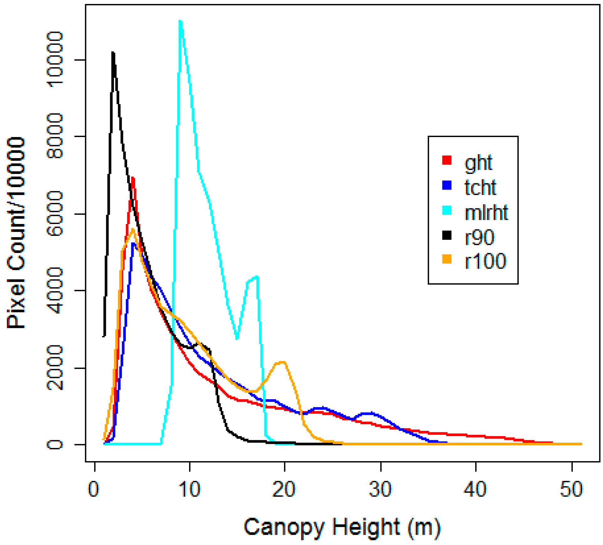
The correlation coefficients for the RT models are listed in
Table 4. These five models were then applied to the full set of geospatial data layers to produce five different FHC maps for Alaska. These were compared and assessed for their suitability for integration into the final Alaska EVH product. Histograms of the canopy height values within the five maps were generated, evaluated, and compared (
Figure 4). These histograms show that the mlrht and r90 estimates of canopy height do not extend beyond the 25 m height range and therefore do not capture the higher end of the range of height measured in the field (
Table 2). The histogram of r100 height estimates shows an unexplained bi-modality in height distribution. Because of these issues, and because they had the highest RT model correlation values as well as high correlations values with the observed plot data, the ght and tcht estimates were identified as best capturing the range of expected canopy height for Alaska and used to generate the final FHC map (
Figure 5). For the FHC map, the tcht and ght maps were integrated based on the slope layer. For slopes > 7°, the tcht data were used, because this method resulted in a slightly improved RMSE when compared to the plots located on steeper slopes than the ght data (7.1 m
vs. 8.5 m). In the remaining areas the ght was used. Finally, all areas not designated as a forested system in the LANDFIRE EVT map were masked out.
Table 4.
Correlation coefficients for the RT models for the five GLAS-derived canopy height versions.
Table 4.
Correlation coefficients for the RT models for the five GLAS-derived canopy height versions.
| | Correlation Coefficient |
|---|
| ght | 0.79 |
| mlrht | 0.75 |
| tcht | 0.82 |
| r90 | 0.66 |
| r100 | 0.72 |
Figure 4.
Plot showing the distributions of the five versions of GLAS-derived height: ght, tcht, mlrht, r90 and r100.
Figure 4.
Plot showing the distributions of the five versions of GLAS-derived height: ght, tcht, mlrht, r90 and r100.
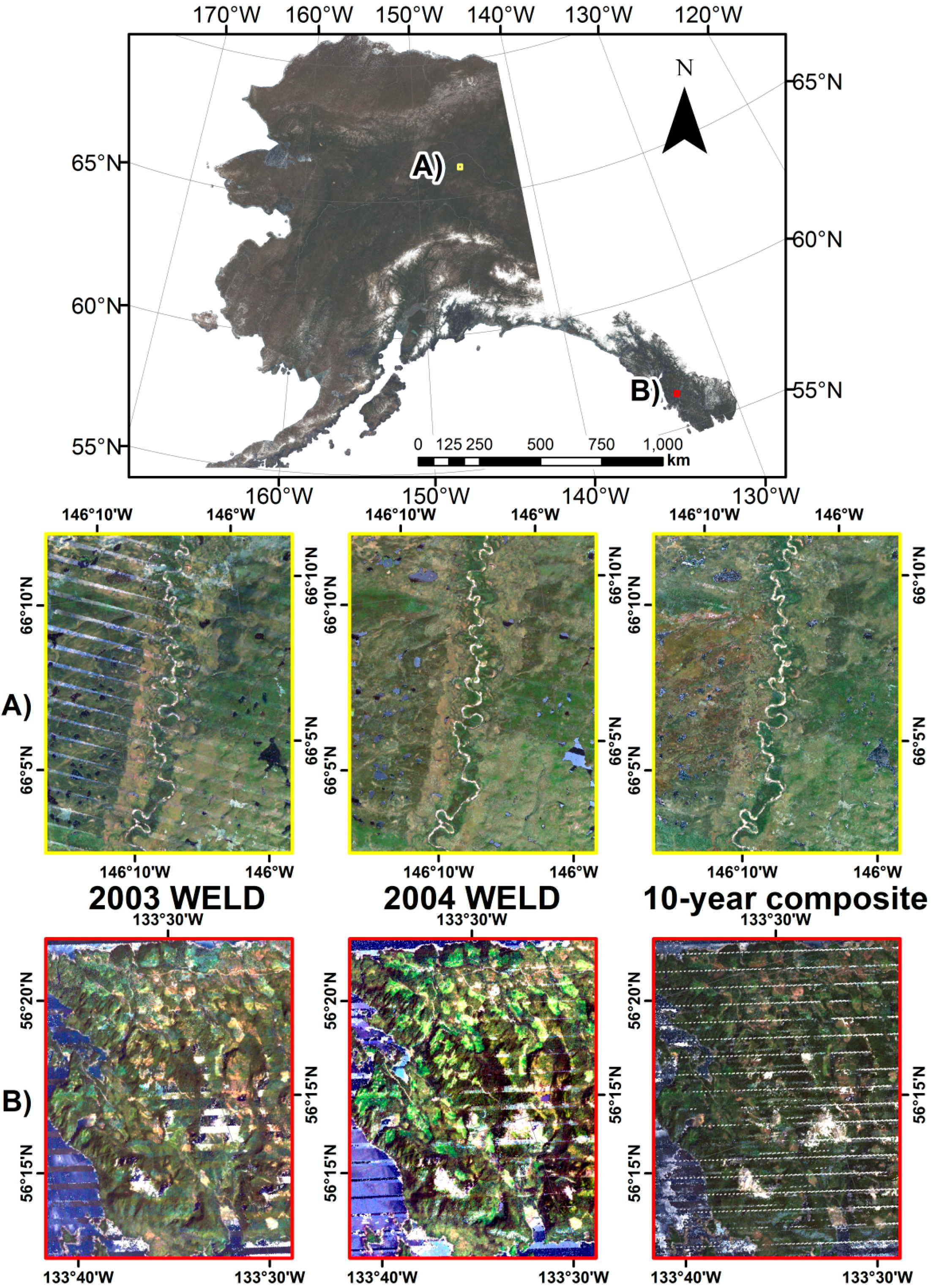
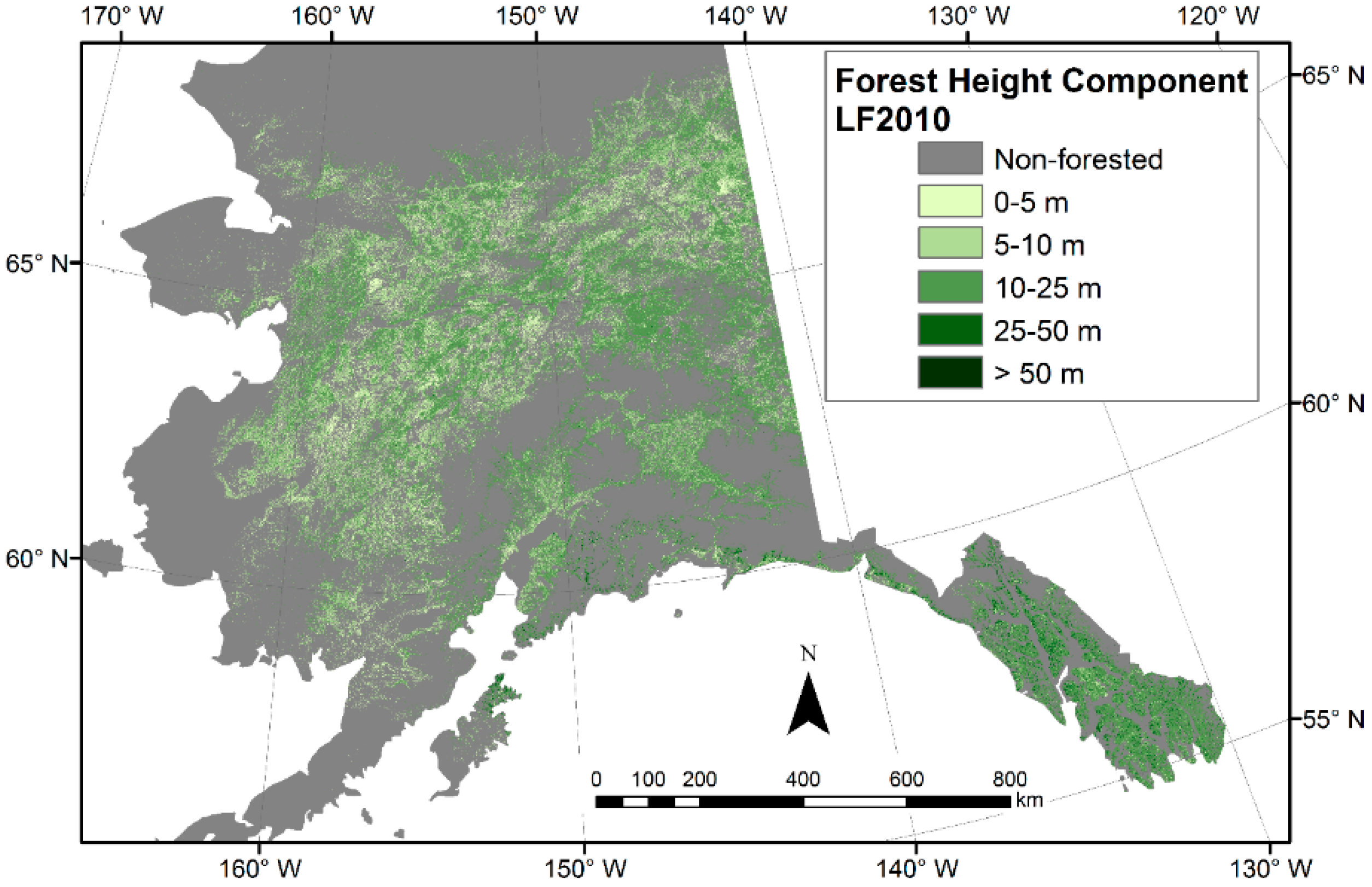
Figure 5.
Updated map of LANDFIRE National forest height component for Alaska mapped as five classes.
Figure 5.
Updated map of LANDFIRE National forest height component for Alaska mapped as five classes.
3.2. Error Assessment
Two confusion matrices describing the relationship between the mapped and observed height values were generated, separating the FIA data from the YRBFD. The confusion matrices are shown in
Table 5 and
Table 6. The mean user’s accuracy over the four classes was 0.26, the mean producer’s accuracy was 0.26, and the overall accuracy was 0.60 for the comparison between the YRBFD and the mapped values. The kappa value was 0.143. The mean user’s accuracy was 0.28, the mean producer’s accuracy was 0.26, and the overall accuracy was 0.54 for the comparison between the field observations obtained from FIA and the mapped values. The kappa value was 0.128.
Table 5.
Confusion matrix for LF2010 EVH and YRBFD.
Table 5.
Confusion matrix for LF2010 EVH and YRBFD.
| YRBFD | LF2010 EVH | Producer’s Accuracy |
|---|
| 0–5 m | 5–10 m | 10–25 m | 25–50 m | Total |
|---|
| 0–5 m | 0 | 2 | 0 | 0 | 2 | 0 |
| 5–10 m | 2 | 3 | 5 | 0 | 10 | 0.30 |
| 10–25 m | 0 | 9 | 26 | 0 | 35 | 0.74 |
| 25–50 m | 0 | 1 | 0 | 0 | 1 | 0 |
| Total | 2 | 15 | 31 | 0 | | |
| User’s accuracy | 0 | 0.2 | 0.84 | 0 | | |
Table 6.
Confusion matrix for LF2010 EVH and FIA data.
Table 6.
Confusion matrix for LF2010 EVH and FIA data.
| FIA | LF2010 EVH | | Producer’s Accuracy |
|---|
| 0–5 m | 5–10 m | 10–25 m | 25–50 m | >50 m | Total |
|---|
| 0–5 m | 2 | 17 | 17 | 1 | 0 | 37 | 0.54 |
| 5–10 m | 3 | 18 | 81 | 4 | 0 | 106 | 0.17 |
| 10–25 m | 8 | 75 | 477 | 90 | 1 | 651 | 0.73 |
| 25–50 m | 3 | 7 | 198 | 100 | 2 | 310 | 0.32 |
| > 50 m | 0 | 0 | 1 | 1 | 0 | 2 | 0 |
| Total | 16 | 117 | 774 | 196 | 3 | | |
| User’s accuracy | 0.13 | 0.15 | 0.62 | 0.51 | 0 | | |
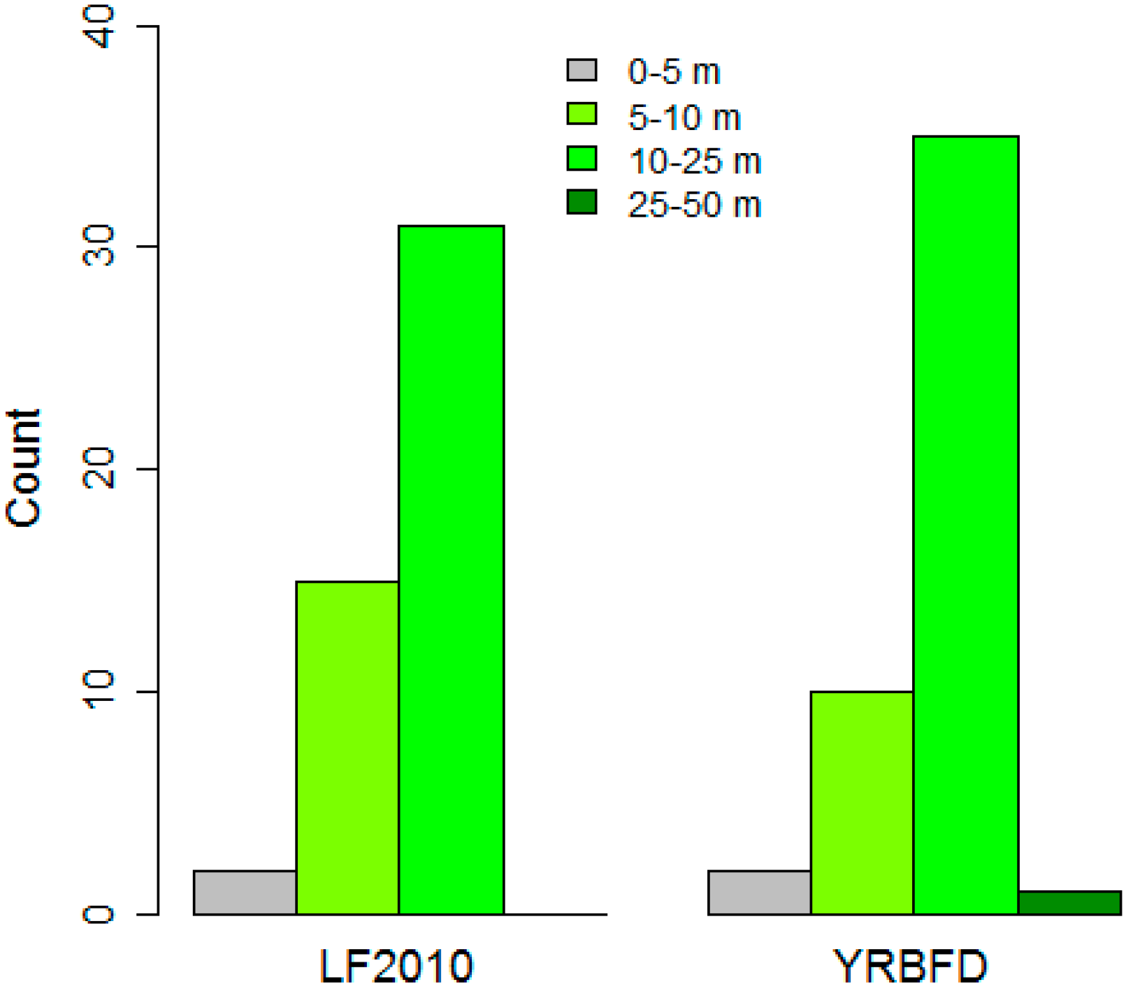
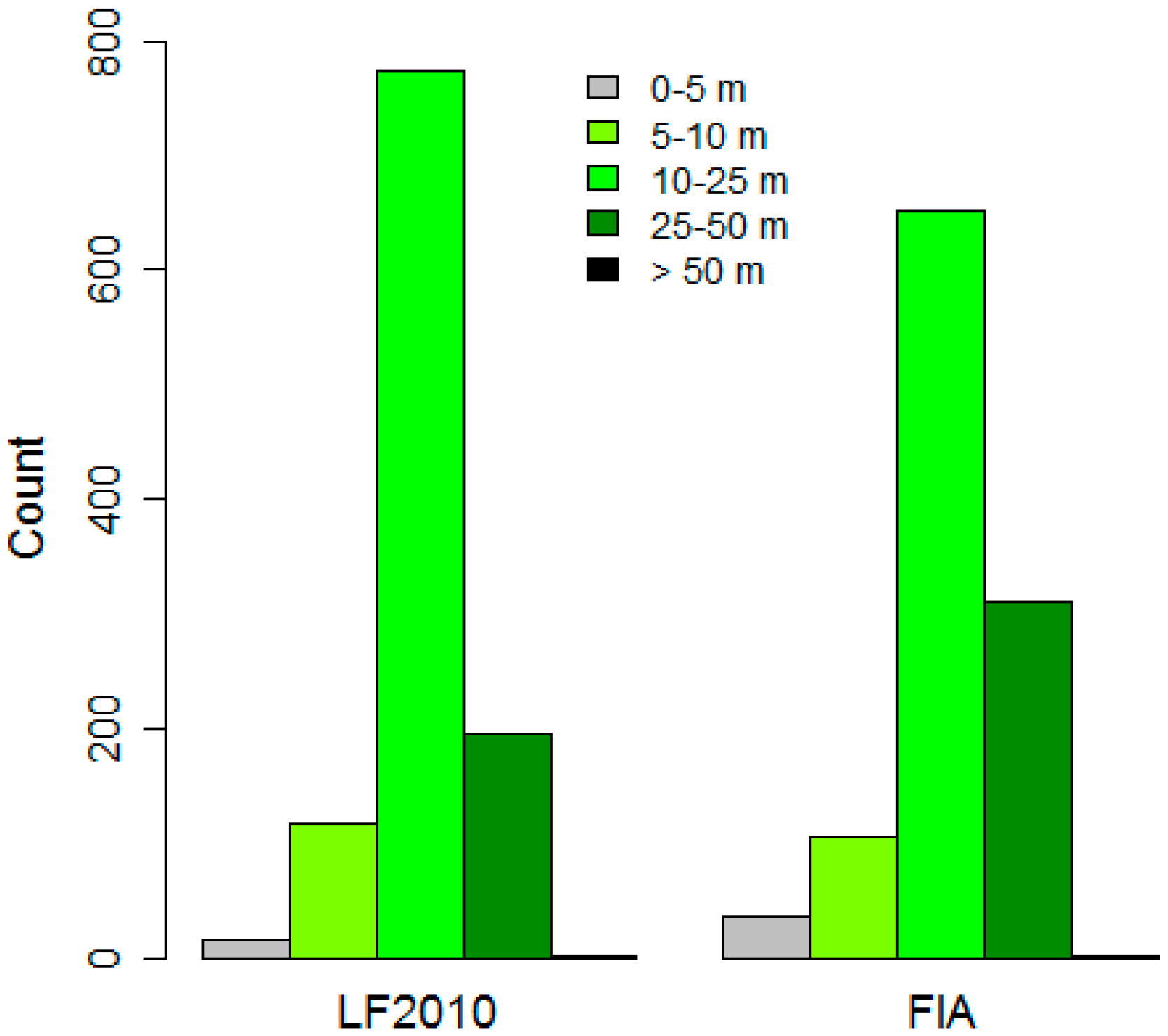
The histograms of the field
vs. mapped data are shown in
Figure 6 and
Figure 7 for the YRBFD and FIA data, respectively. Qualitatively, both histograms show good thematic agreement between the field-observed and mapped data values. However, given the misclassification of heights as indicated by the confusion matrices, this does not indicate that the correct height class was assigned to any given pixel. Still, though the accuracy of the maps is poor at the local scale, they may have good representation at the global scale.
Figure 6.
Histograms of binned FHC derived from the LF2010 mapped canopy height Yukon River Basin field data values.
Figure 6.
Histograms of binned FHC derived from the LF2010 mapped canopy height Yukon River Basin field data values.
Figure 7.
Histograms of binned FHC derived from the LF2010 mapped canopy height FIA field data values.
Figure 7.
Histograms of binned FHC derived from the LF2010 mapped canopy height FIA field data values.
Further work needs to be done to thoroughly understand and quantify the various sources of error underlying the lack of correspondence between the field observations and the mapped canopy height values. The low kappa statistics can in part be attributed to the relatively low sample size. Though the total number of plots included in the assessment is >1000, most of these are the FIA plots that were established in the southeastern part of the state, leaving many regions of the state un-sampled. Furthermore, the total area represented by the plots is very low as compared to the total area mapped. In total only 450 ha of forested lands were sampled of the total 38,000,000 ha. One source of potential error is the configuration represented by the 2010 YRBFD plots. The long, narrow transects represent small areas that can miss sampling taller trees that are actually near the vicinity of the plots. This could lead to an apparent over-estimation of height in the final mapped product assuming these taller stems were reflected in the remote sensing-derived height. Another source of error can be attributed to the low canopy densities in some of the plots. Spruce trees in the YRB often have very narrow, conically-shaped crowns. This represents a small area for LiDAR to reflect off of relative to the total area of the footprint. Substantial penetration of the LiDAR beam into the canopy could occur before a canopy signal can be detected. This would lead an apparent under-estimation of the canopy height relative to the field observation. The high slopes that occur in much of the area where the FIA data were sampled will impact the GLAS-based height estimation, given the reliance solely on waveform extent to map height. However, as LANDFIRE data are intended to be applied at a broader landscape scale, lack of correspondence between field observations and specific pixel values are expected and acceptable, provided regional trends and larger scale patterns align. If LANDFIRE data are being used for local scale analyses, further scrutiny is needed to determine their applicability and they may require editing to meet the needs of the analysis.
There are several limitations to the LF2010 Alaska EVH map. The slope correction attempted here was parameterized using an airborne LiDAR data set that represented a relatively small portion of the state covering a small range of slope conditions. The timeframe for the completion of the Alaska LF2010 map did not allow for the inclusion of LiDAR data sets that could have been used to develop more regionally tuned slope correction coefficients. The validation of the EVH map is incomplete and is limited by a lack of field observations for many of the forested lands within the state. Furthermore, though this process has helped eliminate seamlines caused by scene edges, the exclusive use of Landsat 7 ETM+ data by WELD resulted in scan-gap artifacts in the final product. While attempts were made to mitigate these through the development of the super-composite, minor artifacts are still present and must be accounted for when using the product for fire behavior simulation or other applications. Lastly, to ensure that as many GLAS footprints as possible were included in the analysis, data from all GLAS laser campaigns from September 2003 on were included and processed using the same algorithms. These data were collected over a 5+ year period, and therefore do not reflect a static moment in time, as would data from a single Landsat scene. Because vegetation disturbance is largely limited to wildland fire in Alaska, except in the southern Alaskan forests where insect infestation and timber harvesting also account for significant disturbance, using observations that span such a large timeframe is somewhat mitigated.
3.3. Relevancy and Impacts
Several other studies have used GLAS data to derive canopy height over large regions, but have typically combined them with 250 m resolution MODIS data rather than 30 m resolution Landsat data. These studies typically developed products that are global assessments of canopy height [
25,
26,
27] and do not provide the spatial resolution required by users of LANDFIRE data or do not cover the far northern latitudes. For the LF2010 product, the required resolution was 30 m to match the other datasets in the product suite.
Re-mapping the FHC of the EVH layer has consequences for downstream LANDFIRE data products that rely on vegetation height as an input to their mapping processes. Most notably, the surface and canopy fuel layers are driven in part by the EVH layer. Surface fuel models are assigned using rulesets based on the EVT, EVH, existing vegetation cover, and potential vegetation [
28]. The forest canopy height (CH) is a canopy fuel layer that is derived directly from the EVH for forested pixels, and masked for non-forested pixels. The EVH layer is also used for mapping canopy base height and canopy bulk density layers [
28]. Therefore, the increased thematic resolution of the re-mapped FHC directly affects the assignments of surface fuel models and the mapping of canopy fuels, which has tangible effects on strategic and tactical fire behavior modeling, for which these layers are utilized.
The new LF2010 EVH and CH maps for Alaska have several implications for LANDFIRE data users. Foremost, the refinement of the mapped height classes better reflects the heterogeneity of the landscape (
Figure 8) and will lead to improved fire behavior simulations. The increased thematic detail in the forest height map will also lead to a better representation and quantification of the impacts of change and disturbance in the landscape (
Figure 8). These will also be enhanced by the consistency of the data across the state as well as the lack of seamlines (
Figure 8), compared to the earlier version of the EVH map, which was produced on a zonal basis. While the absolute FHC values indicated in the map need to undergo additional validation, the relative values showing where there are taller
vs. shorter, or structurally complex
vs. homogenous forests will also help in fire behavior and fuel assessments, fire effects monitoring, and other applications such as habitat assessment.
More research needs to be done to address the impacts of slope on height recovery in Alaska using GLAS data. The approach used here did not account for the impacts of slope, possibly because of the range of slopes present in the area of the Kenai ALS data set that was intersected by usable GLAS footprints. Eighty-six percent of these footprints fell in areas that were ≤ 7° in slope. Of the remaining 14%, over half fell onto slopes between 8° and 12°. The steepest slopes were not well represented in the data. Also, the canopy heights derived from the Kenai ALS data were not validated or field verified, so the training data may also have contained errors.
Many of the high-latitude forest systems around the globe are remote and lack the infrastructure to support intense ground- or even air-based sampling and inventory. Space-based remote sensing is the only cost-effective alternative for gathering information about these systems for ecosystem assessment and monitoring. Thus far, the data provided by the GLAS mission represent the only source of consistent LiDAR observations of canopy structure with a sufficient sampling density to promote the mapping of these key variables. This study presents a method for integrating these data into a large-scale mapping effort that can also be applied in other high-latitude ecosystems.
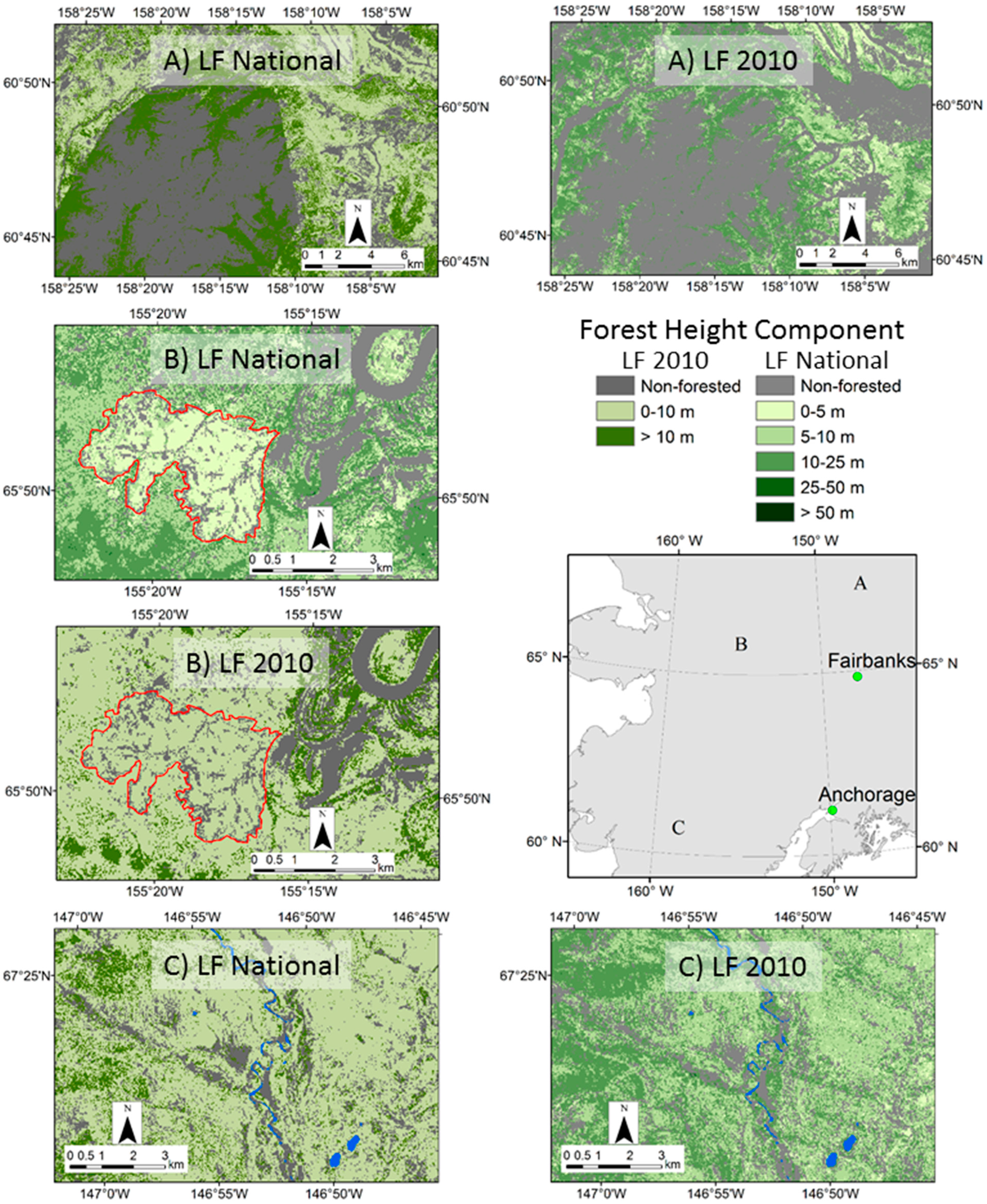
Figure 8.
Examples of qualitative improvements in the LF2010 FHC map vs. LANDFIRE National original. (A) shows an improved representation of a vegetation structure patterns associated with a riparian corridor, (B) shows a better representation of structural change resulting from a fire (burn perimeter shown in red), and (C) shows the mitigation of seamlines using the new method.
4. Conclusions
The incorporation of GLAS data to supplement limited field observations available for mapping in Alaska has improved the utility of the LANDFIRE EVH product and addressed user needs. Specifically, the refinement of the forest height component of the EVH product from two classes to five allows better representation of landscape variability, a critical factor in fire behavior modeling and other ecosystem applications. GLAS data have been used in previous studies to map forest height, however typically globally at a coarser scale. In this study, we demonstrate that they are also useful in mapping more local scales at finer resolution, although subject to the limitations identified herein. This map provides a better understanding of the distribution of forest canopy height across the state of Alaska than was previously available. This increased understanding will enable more detailed fire behavior modeling. Furthermore, it will provide an updated baseline from which disturbance and growth modeling can be captured for assessing ecosystem change. With the end of the GLAS data collection in 2009 no new spaceborne LiDAR data are currently available for updating maps. This study has prepared LANDFIRE for when such data are again available in the future. The ICESat-2 mission, which will provide new spaceborne LiDAR data using the Advanced Topographic Laser Altimeter System, is slated for launch in 2017.


