Article

Trait Estimation in Herbaceous Plant Assemblages from in situ Canopy Spectra

by
Hans D. Roelofsen
1,*,
Peter M. Van Bodegom
2,
Lammert Kooistra
3 and
Jan-Philip M. Witte
1,2
1
KWR Watercycle Research Institute, Groningenhaven 7, P.O. Box 1072, 3430 BB Nieuwegein, The Netherlands
2
Systems Ecology, Department of Ecological science, VU University Amsterdam, De Boelelaan 1085, 1081 HV Amsterdam, The Netherlands
3
Laboratory of Geo-Information Science and Remote Sensing, Wageningen University, Droevendaalsesteeg 3, 6708 PB Wageningen, The Netherlands
*
Author to whom correspondence should be addressed.
Remote Sens. 2013, 5(12), 6323-6345; https://doi.org/10.3390/rs5126323
Submission received: 23 September 2013 / Revised: 7 November 2013 / Accepted: 13 November 2013 / Published: 25 November 2013

Abstract

:
Estimating plant traits in herbaceous plant assemblages from spectral reflectance data requires aggregation of small scale trait variations to a canopy mean value that is ecologically meaningful and corresponds to the trait content that affects the canopy spectral signal. We investigated estimation capacities of plant traits in a herbaceous setting and how different trait-aggregation methods influence estimation accuracies. Canopy reflectance of 40 herbaceous plant assemblages was measured in situ and biomass was analysed for N, P and C concentration, chlorophyll, lignin, phenol, tannin and specific water concentration, expressed on a mass basis (mg·g−1). Using Specific Leaf Area (SLA) and Leaf Area Index (LAI), traits were aggregated to two additional expressions: mass per leaf surface (mg·m−2) and mass per canopy surface (mg·m−2). All traits were related to reflectance using partial least squares regression. Accuracy of trait estimation varied between traits but was mainly influenced by the trait expression. Chlorophyll and traits expressed on canopy surface were least accurately estimated. Results are attributed to damping or enhancement of the trait signal upon conversion from mass based trait values to leaf and canopy surface expressions. A priori determination of the most appropriate trait expression is viable by considering plant growing strategies.

1. Introduction

The functioning of the biosphere is partly determined by the combined impacts of the biochemical and structural characteristics of the plant species it comprises. These characteristics are commonly described by community-mean trait values [1], through which a vegetation community can be studied. This allows for comparison of ecosystems with little to no taxonomic overlap and tends to provide increased insight into plant functioning compared to taxonomic identity alone [2]. In this study, we refer to any biochemical or structural plant property as ‘plant trait’ or simply ‘traits’.
It is recognized that plant traits structurally influence spectral properties of leaves and canopies alike [3,4]. Because these trait-driven nuances in spectral signatures may be obscured by the broad spectral sensitivity of broad band sensors, attention turns to imaging spectroscopy (also known as hyperspectral remote sensing) to register the spectral signal in many small width spectral bands [5]. Small width absorption features have thus been related to various traits, both directly on leaf level (e.g., [6,7]), at canopy level using field spectroscopy (e.g., [810]) as well as at regional scales using airborne imaging spectroscopy (e.g., [11]).
While many different spatial scales have been investigated, in terms of biomes under investigation, especially forest ecosystems appear to receive much attention [12]. Estimation of plant traits in assemblages of naturally occurring herbaceous plant species on the other hand, appears to be less advanced, even though herbaceous environments have a large extent and influence biodiversity, biochemical cycles and fluxes [13]. Remote sensing techniques applied to herbaceous areas so far focused on mapping (temporal changes in) categorical variables, or a limited number of traits, see for a review [3]. In fact, to our knowledge some traits have hardly been, if at all, investigated at all for a herbaceous setting. These include phenol [14], tannin and lignin, which were earlier successfully related to forest canopy reflectance [15].
There are a number of reasons for the limited applications to herbaceous communities. Firstly, the dimensions of herbaceous specimens are typically well below the spatial resolution of imaging spectroscopy [16]. The compound spectral signal in a heterogeneous herbaceous assemblage is thus determined by many different spectral signatures [16,17] that need to be aggregated to a certain community averaged spectral signal. Such aggregation can comprise the footprint of an airborne sensors pixel, or the field of view of a field spectrometer. An advantage of the latter is that the high geometric accuracy (i.e., the spectrometer can be precisely maneuvered over an area of interest), so that the response variable can be measured directly within the sensors field of view.
Secondly, in addition to the leaf biochemical spectral signal, canopy properties unique for herbaceous setting further influence the canopy spectral signal. Previously, litter and canopy height have been identified as a confounding factor between canopy reflectance and species composition [18], but patches of bare soil are also likely to contribute. The latter is likely more conspicuous for herbaceous assemblages compared to forest settings, because herbivory and canopy gaps quickly expose the underlying ground. In all, trait estimation in a mixed composition grassland or herbaceous community with remote sensing has been described as challenging [19]. Finally, establishment of a community trait value is not straightforward, because these, like the canopy spectral signal, can vary greatly among different plants, even over short distances both horizontally as well as vertically within the canopy [20].
The challenge then is to aggregate trait values to a community-mean value that is both ecologically meaningful and corresponds to the functional attributes that are visible to the sensor and thus manipulate the spectral signal. For forests, this community-mean corresponds to the traits of top of canopy leaves, but in a herbaceous plant assemblage, stems or petioles may need to be included too. Moreover, herbaceous systems are less discretely layered than forests, complicating sampling efforts because ‘top of canopy’ is less meaningful. These considerations complicate the analysis of a canopy spectrum vs. a trait value expressing a community-mean attribute.
Despite these challenges, several techniques have been used to estimate community mean trait values of herbaceous vegetation using field spectroscopy spectral data. Often used are empirical, statistical methods where (derivatives of) reflectance data, such as narrow band spectral indices [9,21,22] or continuum removed absorption spectra [23], are related to observed trait values using statistical techniques such as stepwise regression [23,24] or non-linear partial least squares regression (PLSR) [5]. So far, such empirical relations have been found to be poorly transferable between different locations or between different moments at the same location [18], which may be partly related to a lack of considerations on how community-mean traits need to be expressed. In addition, it is noted that often only a few traits are considered within a study [24]. Application of radiative transfer models (RTMs) to herbaceous assemblages is also limited to those traits that are RTM model-parameters, excluding many interesting plant traits [8,2528]. Together, this prevents a direct assessment of how well various traits of herbaceous ecosystems can be estimated.
Furthermore, it is recognized that traits can be expressed relative to different plant properties. This is of relevance for ecological purposes [29], but also for remote sensing [30]. Often, community-mean traits are simply expressed on a leaf mass basis (e.g., [5,23,24]). Alternatively, traits are expressed on a per leaf surface basis (e.g., μg·cm−2 leaf surface, [8]) or per canopy surface basis (e.g., mg·m−2 canopy surface) [8,9]. We will refer to these trait expressions as: mass based, leaf surface based and canopy surface based and indicate the expression with subscript mass, leaf or canopy, respectively. Absence of a subscript refers to all three expressions of a specific trait while all traits in a certain expression are collectively indicated as: ‘mass traits’, ‘leaf surface traits’ or ‘canopy surface traits’, or alternatively as ‘traitmass/leaf/canopy’.
The influence of these trait expressions on remotely sensed trait estimates has never been investigated for more than a few traits (Chlorophyll, N, P or K) and more than two different expressions at the time [8,9,31,32]. No study to our knowledge has compared accuracy of trait estimations for the three trait expressions identified here. Hence, the objective of this study is to examine the overall estimation capability of a wide range of community-mean trait values over various herbaceous assemblages. The secondary objective is to investigate the influence of community trait aggregation, indicated by the different trait expressions, on the estimation capability of the traits. Our approach was to measure in situ canopy spectra, canopy architecture and other plot co-variates and community mean traits (in three expressions) and to investigate the influence of traits of canopy spectra using multivariate regression.

2. Materials & Methods
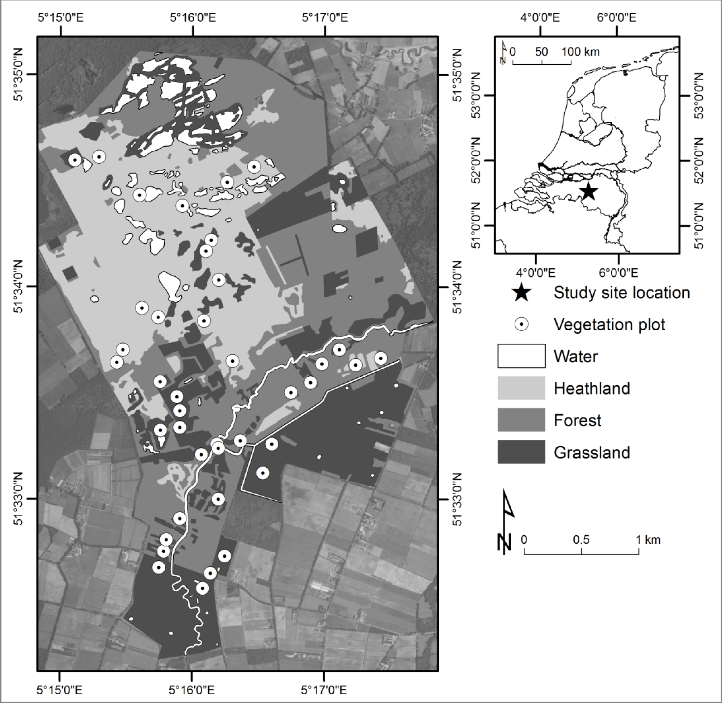
2.1. Study Site

The Kampina Natura2000 protected nature reserve was selected as the study area. It is located on Pleistocene aeolian cover sand landscape in the south of the Netherlands (Figure 1) and hosts a wide variety of herbaceous vegetation types within close proximity to each other. It is easily accessible by foot and within driving range of laboratory facilities. A 15 km2 study site within the Kampina was delineated, aiming to include as much adjacent herbaceous vegetation as possible. The study site hosts dry and generally oligotrophic areas to the north, inhabited by dry heather (dominated by Caluna vulgaris), pine forests and several fens. In the southern region of the study site, a small river valley incises the cover sand and hosts a range of different vegetation types such as moist alder forest, moist heather dominated by Erica tetralix and both mesotrophic and eutrophic moist to wet grasslands. Surrounding agricultural parcels were converted to natural conditions during 2000–2005 by removing the nutrient rich topsoil and raising the groundwater table.

2.2. Data Collection and Processing

2.2.1. Plot Surveying and Floristic Composition

During July and August 2012, 40 plots were sampled in the study site on locations that were manually chosen within strata of broad vegetation types, based on a pre-existing vegetation map [33]. Plot locations were selected to be homogeneous in vegetation composition, without trees or tall shrubs and where ground water was not up to ground surface. Because we are interested in how plant traits manifest in canopy spectral signals, we aimed to have as complete vegetation coverage as possible. Non-vegetated material would also influence the spectral signal, but would not be accounted for in the trait values.
A plot consisted of a patch of homogeneous vegetation, approximately 2 × 2 m, within which several plot characteristics were measured (see following sections for details): location with sub cm. accuracy, floristic composition and coverage, canopy height and Leaf Area Index (LAI, m2 leaf surface·m−2 ground surface, [43]), 10 plant traits and canopy reflectance. Each plot characteristic was measured in a subsequent visit to the plot and care was taken not to take measurements in previously disturbed parts of the plot. Due to the homogeneous vegetation inside each plot we considered all measurements taken from it to be representative for the vegetation in the plot, even when the measurements were not done on the same material.
The plots were distributed over several following broad vegetation types as follows, where n is the number of plots in the type:
  • Dry heathlands, dominated by C. vulgaris, n = 4
  • Moist heathlands, dominated by E. tetralix, n = 5
  • Heathlands with grass encroachment, dominated by Molinia caerulea, n = 4
  • Eutrophic grasslands, former meadows, among others species abundance of Trifolium sp, Holcus lanatus, Agrostis capillaris, n = 7
  • Eutrophic meadows along walking paths, dominated by Phragmitum australis and Utrica dioica, n = 2.
  • Mesotrophic wet grasslands, Cirsium dissectum, Succisa pratensis, n = 5.
  • Eutrophic wet grasslands, Phalaris arundinacea, Carex acuta, n = 4.
  • Mesotrophic, moist, sites within the recently converted agricultural areas, containing among others, Betula sp sapplings, Drosera intermedia, C. vulgaris and Salix repens sapplings, n = 5.
Four plots were dominated by a single species: Juncus effuses, Pteridium aquilinum, Cladium mariscus and Myrica gale, respectively.

2.2.2. Plot Traits

We selected a suite of plant traits that we suspect are instrumental in defining leaf spectral signals and are known to play a key role in plant functioning and plant strategies. These were: leaf N, P and C concentration (LNC, LPC, LCC), Chlorophyll a, Chlorophyll b and total Chlorophylls (Chl a, Chl b and total Chl, collectively referred to as Chl), lignin, tannin, phenol and Specific Water Concentration (SWC). These are traits that are commonly applied in ecology [2] or remote sensing science [15].
Within each plot, vegetation was sampled within a randomly located subplot of 25 × 25 cm. By virtue of this sampling design and plot site selection, trait values are assumed to be representative for an entire vegetation plot. Where possible, the complete above ground biomass was harvested. In case of tall vegetation (>50 cm), the upper ±50 cm was harvested. Woody elements were not sampled because they are incompatible with chemical analysis protocols. The complete sample was manually shredded and homogenized in the field. Subsequently, three subsamples (A–C, approximately 15 g fresh weight material per subsample) were taken from the shredded material and were each stored according to the various prerequisites of the trait determination procedures. A fourth subsample (subsample D) was harvested directly without shredding the sample first. All sampled material was transported to laboratory facilities within 24 h.
Subsample A was analyzed for Specific Water Concentration (SWC, g water·g d.w.−1). Dried plant material was ground and analyzed for Leaf N and Leaf C Concentration (LNCmass, LCCmass, mg·g−1) using dry combustion. Leaf Phosphorus Concentration (LPCmass, mg·g−1) was measured using the method of Murphy and Riley [34]. Finally, ligninmass was determined following Poorter and Villar [35]. Subsample B was analyzed for tanninmass and phenolmass following [36], while from subsample C Chl amass, Chl bmass and total Chlmass concentration was determined spectrometrically using extinction coefficients provided by Porra et al. [37]. The area and dry weight of subsample D was measured to determine the plot Specific Leaf Area (SLA, mm2·mg−1). A detailed account of the sample processing and trait determination procedures, as well as trait summary statistics and correlation, are provided in Supplementary Data 2.

2.2.3. Plot Co-Variates

Several additional variables of the plots were quantitatively assessed to assess the environmental conditions at the plot and to assess the structure of the vegetation. Firstly, the plot floristic composition was recorded based on the entire plot area, including a visual estimation of the % coverage of vegetation and % bare soil. The height in cm of the shrub layer was measured.
Secondly, plot-averaged indicator values (IVs, see Diekmann [38] for a review) were calculated as the average of the IVs of all species in a plot, based on a list of species indicator values from Witte et al. [39]. IVs are an ordinal value indicative of the site’s moisture regime (mF, ranging from 1 = aquatic to 4 = dry), nutrient availability (mN, ranging from 1 = nutrient poor to 3 = very nutrient rich) and acidity (mR, ranging from 1 = acid to 3 = alkaline). Note that we did not employ the original IVs as introduced by [40], but rather a list of IVs per plant species specifically composed for the Netherlands. See Witte, Wójcik, Torfs, De Haan and Hennekens [39] for a detailed explanation of the derivation of the IVs and Roelofsen et al. [41] for a more in depth explanation of IV calculation for vegetation plots. No actual physical measurements were involved when determining plot mean indicator values, which makes this a cheap and quick, but admittedly crude [42], method to gauge the site conditions of a plot.
Finally, the LAI was determined using an LAI2000 instrument (Li-COR Inc, Lincoln, NE, USA, a detailed description of this instrument is provided in Welles and Norman [43]). The sampling protocol consisted of four below canopy measurements, one at each side of the plot, preceded and followed by an above canopy measurement.

2.2.4. Trait Expressions

Traits were expressed in one of three ways: (1) mg·g−1 dry matter (2) mg·m−2 leaf surface and (3) mg·m−2 canopy surface. These trait expressions represent hypothesizes about the interaction of radiation with the canopy. Firstly, mass based traits assume that the complete leaf contributes to the spectral signal, regardless of whether the trait content is apparent at the leaf surface, or tucked away within the leaf. To illustrate, for equal LNCmass value, the amount of N on a given leaf surface can be very different and is determined by the leaf density. Mass based traits are expected to relate well to leaf spectra when radiation fully penetrates the leaf and absorbance is modulated by all trait content within the leaf.
Secondly, leaf surface traits suppose that the field of view of the sensor is fully occupied by a single layer of leaves and that only these leaves contribute to the spectral signal. Hence, only trait content contained in the perceived foliage is presumed to contribute to the spectral signal and non-leaf elements such as woody and dead biomass are expected not to contribute to the signal. Therefore, we may expect this alternative to perform best when nothing but foliage is present in the canopy (i.e., no bare soil or dead material).
Canopy surface traits assume that all foliage contributes to the spectral signal, regardless of whether or not it is in the field of view of the sensor. All leaves contribute to the spectral signal according to this expression via backscattering, oblique reflectance and transmission. If this is the case, then all leaves inside the canopy should also contribute to the community-mean trait value.
The chemical analysis directly yielded mass based trait values. These were expressed on leaf surface and canopy surface basis according to Equations (1) and (2):
trait leaf   ( mg m - 2 leaf   surface )   =   trait mass   ( mg g - 1   dry   matter ) / ( SLA   ( mm 2 mg - 1   dry   matter ) / 1000 )
trait canopy   ( mg m - 2   land   area )   =   trait leaf   ( mg m - 2   leaf   surface )   ×   LAI   ( m 2   leaf m - 2   land   area )
except for SWC for which the numerator is in grams. Note that SWC is related to various other plant traits that are common in ecological or remote sensing applications; SWCmass relates to Leaf Dry Matter Content (LDMC, g dw·g−1 fw, [2]) following Equation (3), while SWCleaf equals Equivalent Water Thickness (EWT, cm3 H2O·cm−2 leaf surface, [44]) and SWCcanopy equals Canopy Water Content (CWC, g H2O·m−2 land area [25]):
SWC mass = ( 1 / LDMC ) 1

2.2.5. Plot Spectra

In each of the 40 plots, canopy reflectance was measured using an ASD (Analytical Spectral Devices, Inc., Boulder, CO, USA) FieldSpec Pro FR spectrometer. Measurements were calibrated against a white Spectralon (Labsphere Inc., North Sutton, NH, USA) panel. Ten spectral measurements were made over each plot. The sampling design was as follows. A single measurement in the center of each 66 × 66 cm square was taken in a 3 × 3 squares array within the boundaries of the plot, finalized by a final single reading over a random location in the plot (comparable to the VALERI sampling scheme [45]). We used a bare optical cable with a viewing angle of approximately 25 degrees, resulting in a field of view with radius 33 cm when held approximately 150 cm above ground surface. Approximately 85% of the plot surface was thus covered. Because spectral measurements in the field require sunny and cloud free circumstances, the spectral measurements were confined to five consecutive sunny and cloud free days in August 2012 between 0900 and 1730 h.
The spectrometer measures spectral radiance between 350 and 2,500 nm, with a sampling interval of 1 nm and spectral resolution of 3 nm in the Visible (VIS, 350–1,700 nm) and Near-Infrared (NIR, 700–1,350 nm) regions and 10 nm the Short-Wave Infrared (SWIR1: 1,450–1,800 nm and SWIR2: 2,050–2,350 nm) regions. Standard preprocessing of the data yields discrete reflectance values for each consecutive nm in the range 350–2,500 nm, but spectral bands with considerable atmospheric absorption were removed (1,350–1,450 nm, 1,800–2,050 nm and 2,350–2,500 nm). The remaining reflectance data were smoothed using a 2nd order Savitsky-Golay filter [46]. Filter length was 7 bands, but increased to 21 bands for a particularly noisy region around 1,000 nm and was increased to 51 bands for two plots to attenuate an atmospheric artifact around 1,120 nm. The 10 measurements of each plot were averaged to a single spectral signature per plot.

2.3. Statistical Data Analysis

To gain a first impression on the relation spectrum-trait we calculated Pearson’s correlation coefficients between each trait and each spectral band. With this we could later check the PLSR models for consistency and evaluate whether the models recognized highly correlating bands. Correlation is described as strong (r > 0.7), moderate (0.5 > r > 0.7) or weak (r < 0.5).
PLSR is an useful technique for relating dependent variables to many, highly correlated, explanatory variables [47]. PLSR reduces the dimensionality of the explanatory variables and projects the information content into new, orthogonal latent variables [47]. The regression is then applied with that number of latent variables (NLV) as explanatory variables that is the optimal tradeoff between complexity and precision, i.e., prevent over-fitting but also achieve optimal accuracy.
The spectral bands were standardized by the standard deviations. Model accuracy was determined twofold: the calibration accuracy tells how well the model is fitted to the training data. Using Leave One Out (LOO) validation, the ability of the model is gauged to estimate trait values for a spectrum that was not present in the training set. For both the calibration and validation, a coefficient of multiple determination (r2) and root mean square error (RMSE) were calculated, indicated with subscript cal and val respectively. The NLVs of the final model is the number that minimizes the RMSEval. However, this criterion could enforce a very high NLV, which immediately generates a high r2cal. In cases where both a low (∼3–4) and high (>8) NLV generated comparable low RMSEval values, the lower NLV was chosen, aiming for model parsimony. PLSR was applied between canopy reflectance and all traits of the 40 plots (10 traits in three different expressions), using both log10 corrected and original trait values, retaining the highest validated (r2val) model. For each of the LOO validation model fittings, the regression coefficients were calculated. A t-test revealed if the mean regression coefficient deviated significantly from 0. A band was considered significant (i.e., stable) if p < 0.05. PLSR models were iteratively fitted by cropping the spectral bands to the significant spectral bands of the prior run. This was repeated until all spectral bands were significant, or until cropping did not result in an improved RMSEval. Band selection could involve up to five model iterations, but only a singly iteration was sufficient for most models.
Model residuals were correlated to plot co-variates: indicator values, vegetation coverage, bare soil, vegetation height and LAI, using Pearson’s correlation coefficient and tested for significance at p = 0.05. All data analysis was performed in R [48], using the pls package [49] and scripts adapted from Feilhauer et al. [50].

3. Results

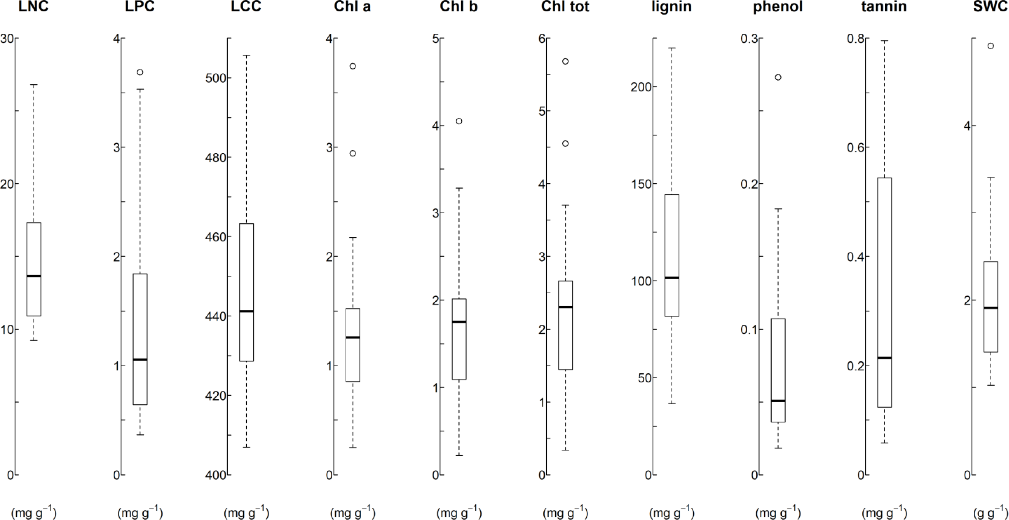
3.1. Traits Values and Plot Co-Variates Reflect Wide Range of Environmental Conditions

The range of trait values reflect the wide variety of environmental conditions, ranging from mesotrophic to oligotrophic sites and of varying moisture levels (Figure 2 and Supplementary Data 2). This is consistent with the sampling scheme that specifically included various vegetation types and abiotic conditions. Correlations among traits are notably high between the three chlorophyll traits and between lignin, phenol and tannin.
In addition to the trait values, the plot co-variates corroborate the impression of a wide variation in environmental conditions present in the plots (Supplementary Data 3). The IVs range from nutrient poor to rich (mN = 1–2.7), very wet to extremely dry (mF = 1.8–3.9) and acidic to alkaline soils (mR = 1.1–2.6). The LAI data confirmed that most plots were densely populated, with only a single plot having an LAI value <1, meaning that leaf surface is less than the ground surface. The highest LAI value (8.31 m2·m−2) was observed for a plot along the eutrophic wet grasslands.
The wide range of traits was planned as to make the relation between traits and spectra as wide and general as possible. So, although the canopy spectra all complied to the general spectral signature of healthy green vegetation, much spectral variation was observed, especially in the NIR range (Supplementary Data 4). Extremes in NIR reflectance were observed in a mesotrophic grassland plot, where high LAI and vegetation height betray a high biomass and an oligotrophic dry heathland where LAI and biomass were relatively low. In the latter plot, the sandy soil may have contributed to the canopy reflectance.

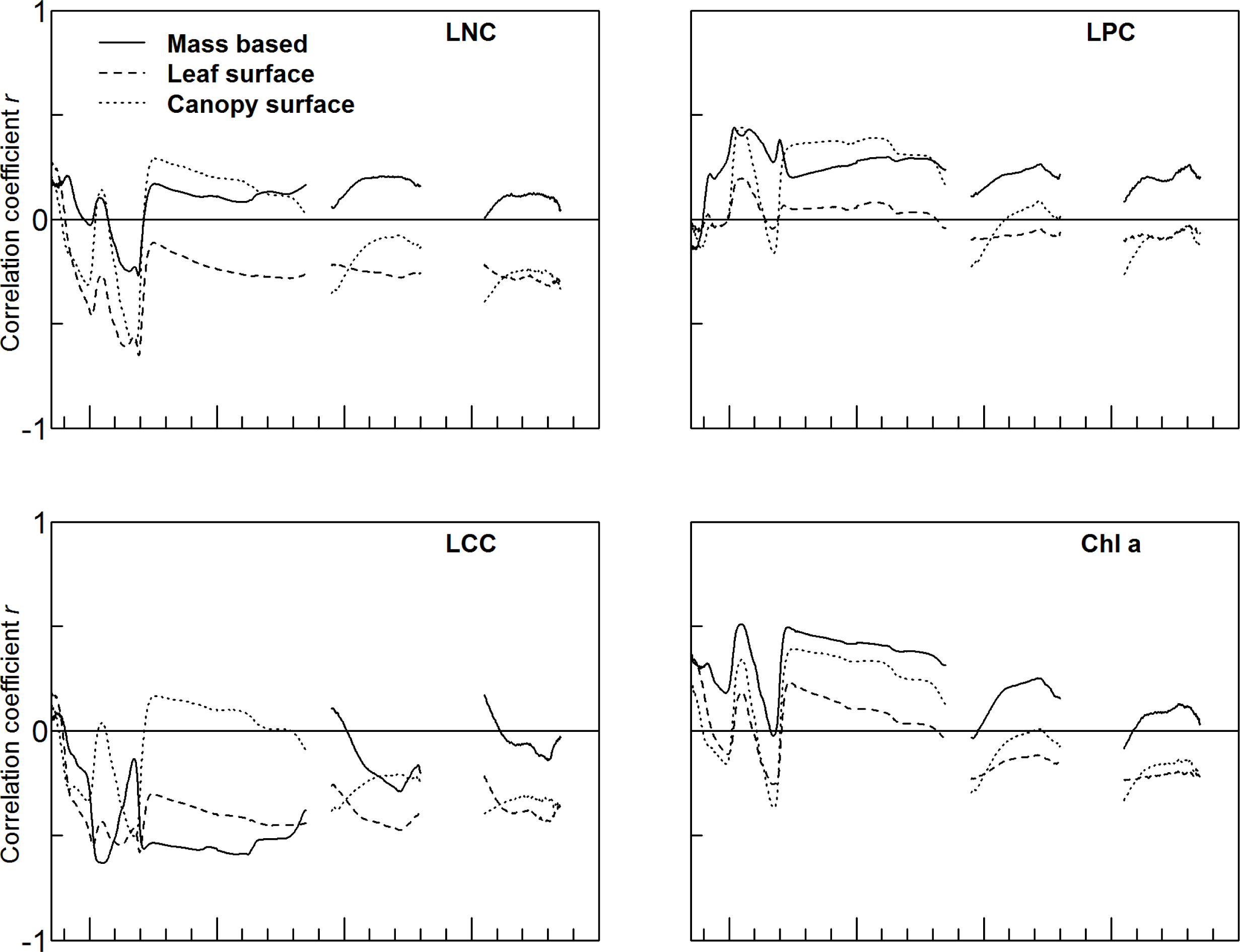
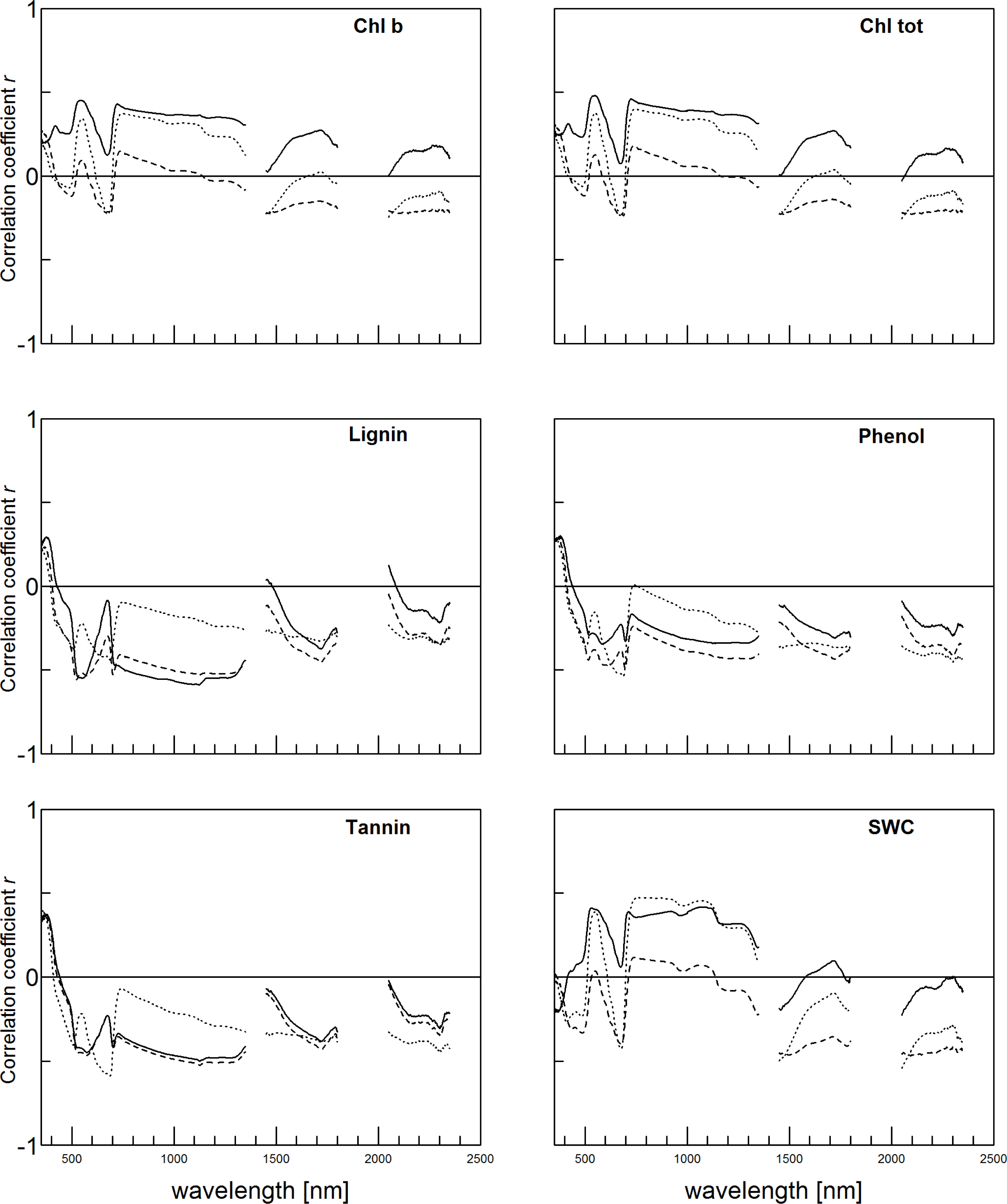
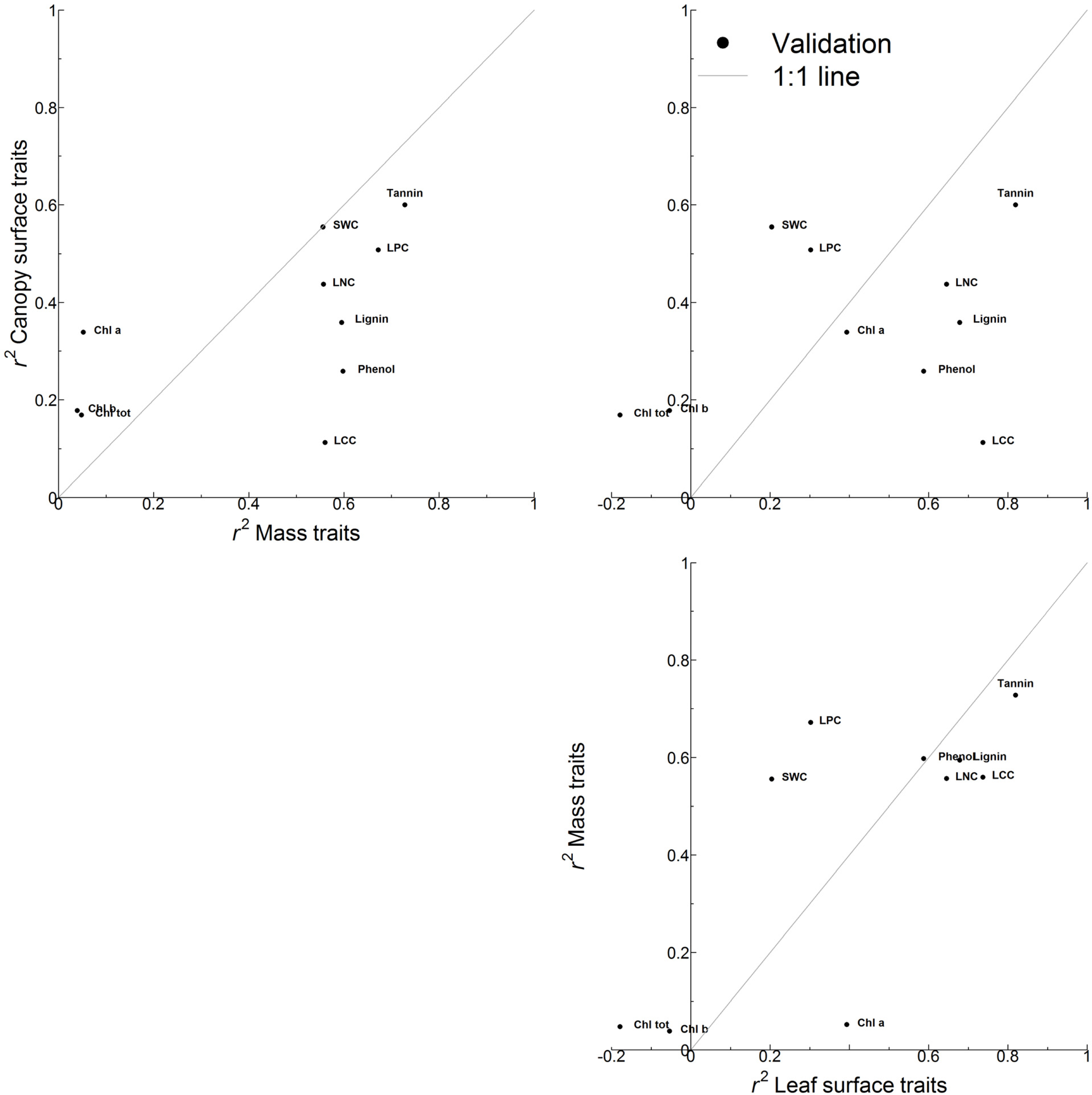
3.2. Accuracy of Trait Estimation Varies with Trait and Trait Expression

The correlation coefficients between spectral bands and leaf surface traits revealed how trait values relate to the various spectral regions (Figure 3 and Supplementary Data 5). Traits with high (high is used in an absolute sense, so either a large positive or negative value) correlation coefficients at certain spectral locations are also expected to be well modeled by PLSR with the PLSR assigning high regression coefficients to these wavelengths.
The VIS region was relevant for nearly all traits. Reflectance around 550 nm correlated strongly to e.g., LCCmass, LCCleaf, all Chlmass and Chlcanopy traits, as well as ligninmass and ligninleaf. The SWIR1 and SWIR2 regions were of low importance for nearly all traits, except for Chlleaf and SWCcanopy. The correlation coefficients for mass, leaf and canopy traits were generally on par, except for some traits where one of the three variants correlated differently (Figure 4). This appears to happen only in the NIR region where correlation between LCCcanopy and NIR reflectance was nearly absent, while LCCmass and LCCleaf correlated reasonably well in that region. Also striking is that LNCleaf correlates negatively with NIR reflectance, while LNCmass and LCNcanopy correlate positively. Likewise, SWCleaf–NIR correlation is virtually zero, but around 0.4 for SWCmass and SWCleaf.
The PLSR regression coefficients between trait and reflectance values (Supplementary Data 5) revealed that for most models VIS reflectance is employed in the model. The location of spectral bands retained in the models generally corresponds to peaks in the correlation coefficients (e.g., for LPCcanopy, tanninleaf and SWCcanopy), although in other cases the PLSR models failed to locate the highest correlating bands (e.g., phenolcanopy around 700 nm and SWCleaf around 700 nm). The pattern of regression coefficients is jagged when a high NLV tightly described the calibration data (e.g., ligninmass NLV = 8). This is indicative of complex, non-linear relations between traits and spectral data (Haaland and Thomas 1988). When fewer latent variables were employed (e.g., total Chlmass NLV = 1), the regression coefficients followed a much more smooth pattern. When band selection did not improve the model accuracy, or when none of the bands was significant, all bands were retained (e.g., phenolleaf). Up to 10 NLV were employed over the PLSR models. Poorly validated models were often signaled by a low NLV (e.g., phenolcanopy, Chl bleaf and total Chlleaf, with 2, 1 and 1 NLV respectively). For nearly all PLSR models, band selection generated a reduced difference between the r2cal and r2val. For three models, none of the spectral bands was found to be significant (total Chlleaf and LCCcanopy) and for five other models, band selection did not result in a more accurate model (LPCleaf, ligninmass, phenolleaf, tannincanopy and SWCleaf).
The resulting accuracy of the PLSR models varied (Figure 4 and Supplementary Data 6) among the traits, among different trait expressions and between the calibration and validation phase. Only validation accuracies are mentioned here, calibration accuracies are provided in Supplementary Data 6. Lignin, phenol and tannin were accurately modeled and validated when expressed on a mass or leaf surface basis, but accuracy degraded once expressed on canopy surface basis. The nutrient related traits (LNC, LPC and LCC) correlated moderately strong with spectral data with r2val up to 0.74. Accuracy of Chl a, Chl b and total Chl estimations was overall low. Negative r2val values were recorded for validation of Chl bleaf and total Chlleaf, meaning that the mean of the observed value was a better estimator than the PLSR model. Chl a always performed slightly better than the other two Chl traits.
Only LNC and tannin retained comparable accuracies regardless of how they were expressed (Figure 4 and Supplementary Data 6). For most traits, the expression greatly influenced the accuracy of the modeling: e.g., LCCcanopy was much less accurately estimated than LCCmass and LCCleaf. None of the different trait expressions clearly distinguished itself by consistently yielding the highest accuracies, although the expression on leaf surface basis most often generated the most accurate models (for LNC, LCC, Chl a, lignin and tannin). Mass based trait expressions generated the most accurate model for phenol, while traits expressed on canopy surface basis yielded most the accurate models for Chl a, Chl b SWC.

3.3. Plot Covariates May Be Additional Drivers of Canopy Reflectance

Correlations, significant at p < 0.05, between PLSR model residuals and plot co-variables are indicated in Table 1. Relatively few mass based and leaf surface traits correlate significantly with plot co-variables, at least few when compared to canopy surface traits of which residuals of five out of 10 trait models correlated with plot co-variables.
Indicator values of site environmental conditions correlated negatively with residuals of three models. Moderately strong correlations were observed with LAI and height, mainly for canopy surface traits. Plot vegetation height and LAI were positively correlated (Supplementary Data 3), explaining why these two plot co-variable often correlated simultaneously with model residuals.

4. Discussion

4.1. Trait Estimation in Herbaceous Plant Assemblages Appears Feasible

The first objective of this study was to estimate community-mean traits over various herbaceous plant assemblages, using in situ measured hyperspectral reflectance. All traits had been investigated earlier in terms of their spectral signatures, but to the best of our knowledge, some of the traits not yet in herbaceous ecosystems (i.e., lignin and tannin). Moreover, a comparison of estimations across a wide variety of community-mean traits of herbaceous communities was so far unavailable. This study demonstrates that, with varying accuracy, various traits can be estimated with a straightforward statistical approach over a wide range of herbaceous assemblages.
Evaluating trait expressions from hyperspectral reflectance is of importance because trait estimation in assemblages of herbaceous species faces particular difficulties [19]. The canopy spectral signal is not only driven by leaf biochemistry, but also by litter and bare soil. These factors contribute to the canopy spectral signal but are not represented in trait values, because solely plant material is accepted by wet-chemistry trait protocols. It is known that at least height and litter fraction influence statistical relations between canopy reflectance and species composition in herbaceous ecosystems [18]. The positive correlations between canopy height, bare soil and vegetation coverage and residuals of eight PLSR models (Table 1) suggest these are indeed consistently confounding factors in the spectrum-trait relation. However, a more detailed experiment is required to quantify the effect of non-vegetation elements in herbaceous plant assemblages on community-mean trait estimation.
An adequate sampling protocol in herbaceous sites is also faced with the problem that plant materials contributing to the spectral signal are less obvious. Especially for graminoids, whose vertically orientated leaves constitute a substantial portion of the plot biomass and thus to the trait value, but of which the nadir surface area and contribution to the spectral signal, may be proportionally low. In this study, we collected plant material throughout the vertical component of the canopy, assuming that (1) both upper and lower canopy material contribute to the spectral signal, due to gaps between the tallest species that expose underlying plants and (2) that the trait content was homogeneously distributed throughout the vertical canopy dimension. Our results do not allow explicit testing of these assumptions due to the homogenization of the sample material. Dedicated sampling and trait determination from different vertical canopy positions and working out various weighted trait averages would shed more light on the question of how various canopy components together compile the overall canopy reflectance.
Nonetheless, this relatively straightforward sampling approach still yielded trait values that relate well to the spectral data, which is critically important for estimating community-mean traits of herbaceous ecosystems. This was apparent from the correlation coefficients between the trait values and individual bands, as well as from the performance of the PLSR models (Figure 3). The accuracy of the estimations was considerably different among the traits. Traits relating to nutrient availability (LNC, LPC and LCC) were well estimated when expressed on either mass or leaf surface basis. This is in line with earlier work, where these traits were also expressed on a mass basis and had comparable or slightly lower estimation accuracies [23,32]. Trait estimation accuracy for these traits may increase when the set of explanatory variables is expanded from solely reflectance to derivatives from reflectance data [24] or additional environmental variables [5]. Given the apparent influence of plot co-variables such as coverage and LAI (Table 1), trait estimations might be further improved by explicitly including these factors into the explanatory variables.
The Chl estimations were among the models with lowest accuracies. This was against expectations, because there is a mechanistic relation between Chl concentration and absorbance in VIS spectra and reflectance in NIR [51]. In fact, leaf chlorophyll content (μg·cm−2 leaf surface) is employed as driver of leaf reflectance in the PROSPECT leaf optical properties model [52] and many studies accurately derived chlorophyll concentration using empirical models and leaf and canopy spectra [7,9,53] or with mechanistic leaf and canopy reflectance models [8]. These chlorophyll estimations rely on the strong correlation with the red-edge (680–780 nm) [54]. Together with green wavelengths (around 550 nm), these spectral regions indeed hosted the highest correlation coefficients of Chlmass and Chlcanopy in the current study (Figure 4), although these were never high in comparison to other traits (i.e., not exceeding r = 0.5). Still, this does not necessarily prevent an accurate PLSR model, as e.g., LNCmass had equally low correlation coefficients but was still modeled moderately accurate. For Chl, it appears that reflectance at 550 nm (one of the highest correlating wavelengths) saturates with increasing Chlmass concentration (data not shown). Therefore, an exponential function might describe Chlmass concentration more accurately than the linear PLSR modeling applied here. Indeed, in Hansen and Schjoerring [9], performance of an exponential model between narrow band vegetation indices and chlorophyll content outperformed a linear model. We did not pursue this option because we restricted ourselves to the simplest, but still physically meaningful model, which is a linear model.
Phenol, tannin and lignin were nearly always strongly to moderately accurate estimated from the spectral data. Two distinct groups are observed in the tannin values and to a lesser extent also for lignin; relatively high values were found in both moist and dry heathland plots, as well as the M. gale and P aquilinum plots. High tannin and lignin concentration is indicative for sturdy and woody leaves and stems, indeed, as found for the various heathland species. Tanninleaf, tanninmass and ligninleaf are among the highest validated models in this study, achieving much higher accuracy compared to earlier estimations based on leaf level spectra [15]. The shrub-like structured and woody components containing canopy of the heathland plots possibly create a distinctive spectral signature compared to grass and herbaceous sites [26], which is sufficiently distinctive to spectrally discriminate the plots with relatively high lignin and tannin concentration from the remaining plots. Canopy physiology and structure, which are known propellants of canopy reflectance [18], might thus have co-varied with tannin and lignin values and are responsible for the highly accurate tannin and lignin estimations. Future studies will need to evaluate these patterns. Accuracy of SWCcanopy estimates was on par with CWC estimation based on PROSAIL model inversion [25].
We used LOO validation, but admit that a stricter validation procedure with an external validation dataset would have yielded a more reliable indication of model robustness. However, our dataset is already characterized by a small sample size (40) compared to a large number of explanatory variables (1,648). A reduced sample would only increase this and likely result in a weaker model as the trait and spectral variability might not be fully covered by the reduced calibration dataset. Repetitively selecting a new random calibration and validation set was considered not feasible because the model calibration process was not automatized. Applying LOO validation on the other hand allowed us to retain the spectral and trait variability [50]. Also, we aimed for model parsimony by restricting the NLV and a reduced calibration sample would have created an unrealistic constrain on the NLV.
Furthermore, we aimed to find out if a relation between spectra and traits existed, and LOO suffices to answer this question. An external validation set is particularly useful after model transfer to other locations, such as in future spatial trait estimations based on imaging data.

4.2. Alternative Expressions of Trait Aggregation

The second objective of this research concerns the aggregation of trait values to a community mean that both corresponds to the aggregated canopy reflectance and is ecologically meaningful. Three alternative trait expressions were related to canopy reflectance: mass based (mg·g−1), leaf surface based (mg·m−2 leaf surface) and canopy surface based (mg·m−2 canopy surface). None of the trait expressions was unequivocally better in relating traits to reflectance (Figure 4). Mass based and leaf surface trait expressions generated model accuracies in the same order of magnitude, while estimates of traits expressed on canopy surface were generally less accurate. This suggests that canopy reflectance is not generated by the entire leaf surface, as was implicitly assumed with the canopy surface trait expression. Rather, results suggest that reflectance originates from leaves in the direct field of view of the sensor.
Still, trait expression on a canopy surface basis yielded the most accurate models for SWC, Chl b and total Chl. Especially for the latter two, the difference with mass based and leaf surface based expressions was large. However, because the overall accuracy of these models was still low (r2val = −0.18 − 0.17 for Chl b and total Chl, Figure 4 and Supplementary Data 5), these results should be interpreted with care. Nonetheless, our results are corroborated by earlier work where chlorophyll content per canopy surface unit was estimated more accurately compared to content per leaf surface [8,21]. These results were attributed to the fact that Chlcanopy traits convey information on both LAI and chlorophyll content, which are both known drivers of canopy reflectance [55]. While this plausibly explains why Chl bcanopy, total Chlcanopy and SWCcanopy were more accurately estimated when expressed on canopy surface basis then on leaf surface, it leaves the question why the remaining traits perform poorer when expressed on canopy surface basis.
Canopy surface traits are the result of multiplying traitleaf values with LAI; hence traitcanopy values and LAI are positively correlated (Supplementary Data 2). An improved relation with canopy reflectance is anticipated if the canopy spectral reflectance is also positively related to LAI. However, any factor that causes the spectral signal to be non-linearly related to LAI will deteriorate the traitcanopy–reflectance relation. Increased scattering by the internal canopy architecture is an example of this. Saturation of the spectral signal with increasing LAI has also been reported [7,9] and may have occurred here as well. We noticed that for LNC, LCC, lignin, phenol and SWC, the PLSR model residuals correlated positively with either LAI and/or canopy height when expressed on a canopy surface basis (Table 1). In other words, estimation accuracy deteriorated with increasing LAI and indeed, these traits are more (or equally, in case of SWC validation) accurately estimated when expressed on mass or leaf surface basis. With increasing LAI, the probability grows that a leaf is obscured by its more elevated counterparts. We hypothesize that obscured leaves contribute less, if at all, to the spectral signal. At the same time, the entire leaf surface contributes to traitcanopy values, so that the discrepancy grows between what is perceived by the sensor and what the canopy surface trait value is suggesting should be there.
Whether either the saturation/scattering effects or rather added information effects of LAI prevail is likely trait-dependent. This may explain the differences between the various traits in this study. The magnitude with which traitleaf values are transformed to traitcanopy values (because LAI > 1 for all plots except one, conversion from traitleaf to traitcanopy nearly always implies an increase in numerical value) depends on the relation between traitleaf and LAI (Supplementary Data 2). A negative relation dampens the traitcanopy signal as low traitleaf values are multiplied with high LAI and high traitleaf values with low LAI. A contracted range of traitcanopy values means that plots become more similar in its community-mean traitcanopy values, while the spectral diversity is retained, thus weakening the spectrum–traitcanopy relation. A positive relation on the other hand increases variation in traitcanopy values, possible enhancing the relation with the spectral data.
Both amplification and dampening of the traitcanopy signals has indeed been observed in the results. A significant (p < 0.05) correlation is observed for phenolleaf and tanninleaf with LAI (r = −0.40 and −0.44 respectively, Supplementary Data 2). This coincides with lower validation accuracy when expressed on canopy surface basis than either leaf surface or mass basis. For the remaining traitleaf, correlations with LAI are non-significant. This lack of relation between the trait and LAI can result in either an amplified signal (i.e., higher estimation accuracy for traitcanopy compared to traitleaf for: LPCcanopy, Chl bcanopy, Total Chlcanopy and SWCcanopy), or a slightly reduced signal.
In a similar fashion, a positive relation between SLA and traitmass works to condense the value distribution of traitleaf, as high traitmass values are divided by equally high SLA values and low traitmass values by a low SLA. This appears to be the case for LPCmass and SWCmass (correlation with SLA r = 0.62 and 0.43 respectively, p < 0.05, Supplementary Data 2); traits which were more accurately modeled when expressed on a mass basis compared to expression on a leaf surface basis (Figure 4). In contrast, LCCmass, ligninmass, phenolmass and tanninmass correlated negatively with SLA (r = −0.42, −0.48, −0.39 and −0.47 respectively, p < 0.05, Supplementary Data 2), so that the leaf surface expression of these traits is an amplification of the mass based trait values. As a result, these traits are estimated more accurately on leaf surface basis compared to mass basis, or at least with accuracy comparable to expression on mass basis (Figure 4).
Chl appears insensitive to both SLA and LAI in our data (i.e., low correlation coefficients, see Figure 3 in Supplementary Data 2). However, this was probably caused by a single plot that combined a low SLA value with the highest Chlmass values and therewith sharply contrasted the more common combination of low SLA and low Chlmass values. Additional research should demonstrate if and how Chl responds to changes in SLA and LAI in different ecosystems, so that the most appropriate expression of Chl be determined.
Overall, we observed that the nature of the relation between traitmass values and SLA, as well as the relation with traitleaf values with LAI influences the estimation accuracies. Furthermore, we reckon that the nature of this relation is, at least partly, determined by the ecosystem. This should be exploited to determine a priori the most appropriate trait expression for each trait. For example, high concentrations of traits such as lignin, phenol and tannin are indicative of investments in defensive structure and indicate tough, long living and slow growing leaves and is incompatible with a high SLA [56]. This negative relation between defensive traits and SLA implies an amplified trait signal when expressed on a leaf surface basis and possibly enhanced estimation capabilities from spectral data. Similarly, competitive species who invest many nutrients in rapid growth after e.g., a mowing event, are associated with high nutrient concentration (LNC, LPC and LCC) and high SLA [57]. Such positive correlation between trait values and SLA suggests that traits should be expressed on mass basis rather than leaf surface. On the other hand, competitive species are also associated with high LAI values due to their rapid growth. The traits related to nutrient content expressed on leaf surface basis could thus be again be amplified by the LAI.

4.3. Implications for Trait Estimations in Herbaceous Ecosystems

The above analyses and interpretations indicate that aggregation of trait values to a meaningful community average is an important issue to consider for spectral estimation of plant traits and should be taken into consideration in future trait estimates. Based on expected relations between trait values and leaf and canopy properties (i.e., SLA and LAI), it is feasible to estimate which aggregation is most appropriate for a trait in a given herbaceous environment. With that, we can move forward to regional estimates of nutrient related traits in herbaceous plant assemblages, which would be beneficial for e.g., rangeland and pasture quality management [23], while chlorophyll estimates would enhance understanding of photosynthetic processes, as well as monitoring foliar condition [51]. Likewise, regional estimates of lignin tannin and phenol could aid research into herbivore pressure and decomposition rates, as well as wildfire occurrence when combined with dry matter estimates [58,59]. In all, regional trait estimates from remote sensing sources can be instrumental in providing input for estimating vegetation composition and functioning [60].

5. Conclusions

The objectives of this research were to examine the overall estimation capability of in situ measured community-mean trait values over various herbaceous assemblages, as well as to investigate the influence of community trait aggregation on the estimation capability of the traits. This study simultaneously estimated 10 different traits of high ecological relevance, some of which were never estimated earlier in herbaceous settings. The importance of trait expressions has been recognized in plant ecology studies, but until this point had not been comprehensively investigated from a remote sensing point of view. Given that canopy surface based traits (i.e., mg·m−2 land surface) hardly produced accurately validated models (0.04 < r2 < 0.60), we conclude that the total trait content per unit ground area is not conveyed to the canopy spectral signature. Instead, the higher estimation accuracy of traits expressed on mass (mg·g−1 dry matter, 0.04 < r2 < 0.73) or leaf surface basis (mg·m−2 leaf surface, −0.18 < r2 < 0.82) suggest that that canopy reflectance is a composition of reflectance from the leaf surface within the field of view of the sensor and from scattering within the leaf tissue. Aggregation of trait values to an ecological meaningful community-mean value that also relates well to the canopy spectral signal is thus not straightforward and depends on the trait in question. However, we found that ecological theory on how trait values relate to Leaf Area Index (m2 leaf surface·m−2 land area) and Specific Leaf Area (mm2·mg−1) provides a priori insight into which trait expression is most appropriate. This might aid future studies on trait estimations in herbaceous plant assemblages, and other ecosystems, to consider trait expressions beforehand.

Supplementary Information

remotesensing-05-06323-s001.pdf

Acknowledgments

We would like to thank Erwin de Hoop (Natuurmonumenten) for allowing access to the Kampina area. Several field work assistants are acknowledged, as well as Harm Bartholomeus (WUR), Rutger Barendse & Philip Wenting (WUR) for technical field work assistance and Rob Broekman (VU), Richard van Logtestijn (VU), Jurgen van Hal (VU) and Anne-Marie van den Driessche (WUR) for the laboratory work. This study was conducted as part of the joint research program of KWR Watercycle Research Institute.

Conflicts of Interest

The authors declare no conflict of interest.

References and Notes

  1. Lavorel, S.; Garnier, E. Predicting changes in community composition and ecosystem functioning from plant traits: Revisiting the holy grail. Funct. Ecol 2002, 16, 545–556. [Google Scholar]
  2. Pérez-Harguindeguy, N.; Díaz, S.; Garnier, E.; Lavorel, S.; Poorter, H.; Jaureguiberry, P.; Bret-Harte, M.S.; Cornwell, W.K.; Craine, J.M.; Gurvich, D.E.; et al. New handbook for standardised measurement of plant functional traits worldwide. Aust. J. Bot 2013, 61, 167–234. [Google Scholar]
  3. Svoray, T.; Perevolotsky, A.; Atkinson, P.M. Ecological sustainability in rangelands: The contribution of remote sensing. Int. J. Remote Sens 2013, 34, 6216–6242. [Google Scholar]
  4. Ustin, S.L. Remote sensing of canopy chemistry. Proc. Natl. Acad. Sci. USA 2013, 110, 804–805. [Google Scholar]
  5. Ramoelo, A.; Skidmore, A.K.; Cho, M.A.; Mathieu, R.; Heitkönig, I.M.A.; Dudeni-Tlhone, N.; Schlerf, M.; Prins, H.H.T. Non-linear partial least square regression increases the estimation accuracy of grass nitrogen and phosphorus using in situ hyperspectral and environmental data. ISPRS J. Photogramm. Remote Sens 2013, 82, 27–40. [Google Scholar]
  6. Curran, P.J.; Dungan, J.L.; Macler, B.A.; Plummer, S.E.; Peterson, D.L. Reflectance spectroscopy of fresh whole leaves for the estimation of chemical concentration. Remote Sens. Environ 1992, 39, 153–166. [Google Scholar]
  7. Doughty, C.E.; Asner, G.P.; Martin, R.E. Predicting tropical plant physiology from leaf and canopy spectroscopy. Oecologia 2011, 165, 289–299. [Google Scholar]
  8. Darvishzadeh, R.; Skidmore, A.; Schlerf, M.; Atzberger, C. Inversion of a radiative transfer model for estimating vegetation lai and chlorophyll in a heterogeneous grassland. Remote Sens. Environ 2007, 112, 2592–2604. [Google Scholar]
  9. Hansen, P.; Schjoerring, J. Reflectance measurement of canopy biomass and nitrogen status in wheat crops using normalized difference vegetation indices and partial least squares regression. Remote Sens. Environ 2003, 86, 542–553. [Google Scholar]
  10. Clevers, J.G.P.W.; Kooistra, L. Using hyperspectral remote sensing data for retrieving canopy chlorophyll and nitrogen content. IEEE J. Sel. Top. Appl. Earth Obs. Remote Sens 2012, 5, 574–583. [Google Scholar]
  11. Knox, N.M.; Skidmore, A.K.; Prins, H.H.; Asner, G.P.; van der Werff, H.; de Boer, W.F.; van der Waal, C.; de Knegt, H.J.; Kohi, E.M.; Slotow, R. Dry season mapping of savanna forage quality, using the hyperspectral carnegie airborne observatory sensor. Remote Sens. Environ 2011, 115, 1478–1488. [Google Scholar]
  12. Knyazikhin, Y.; Schull, M.A.; Stenberg, P.; Mõttus, M.; Rautiainen, M.; Yang, Y.; Marshak, A.; Carmona, P.L.; Kaufmann, R.K.; Lewis, P. Hyperspectral remote sensing of foliar nitrogen content. Proc. Natl. Acad. Sci. USA 2013, 110, E185–E192. [Google Scholar]
  13. Wallace, O.C.; Qi, J.; Heilma, P.; Marsett, R.C. Remote sensing for cover change assessment in southeast arizona. J. Range Manage 2003, 56, 402–409. [Google Scholar]
  14. Skidmore, A.K.; Ferwerda, J.G.; Mutanga, O.; Van Wieren, S.E.; Peel, M.; Grant, R.C.; Prins, H.H.; Balcik, F.B.; Venus, V. Forage quality of savannas—Simultaneously mapping foliar protein and polyphenols for trees and grass using hyperspectral imagery. Remote Sens. Environ 2010, 114, 64–72. [Google Scholar]
  15. Asner, G.P.; Martin, R.E. Canopy phylogenetic, chemical and spectral assembly in a lowland amazonian forest. New Phytol 2011, 189, 999–1012. [Google Scholar]
  16. Verrelst, J.; Geerling, G.W.; Sykora, K.V.; Clevers, J.G.P.W. Mapping of aggregated floodplain plant communities using image fusion of casi and lidar data. Int. J. Appl. Earth Obs. Geoinf 2009, 11, 83–94. [Google Scholar]
  17. Schmidt, K.S.; Skidmore, A.K.; Kloosterman, E.H.; Van Oosten, H.; Kumar, L.; Janssen, J.A.M. Mapping coastal vegetation using an expert system and hyperspectral imagery. Photogramm. Eng. Remote Sens 2004, 70, 703–715. [Google Scholar]
  18. Feilhauer, H.; Schmidtlein, S. On variable relations between vegetation patterns and canopy reflectance. Ecol. Inf 2011, 6, 83–92. [Google Scholar]
  19. Röder, A.; Kuemmerle, T.; Hill, J.; Papanastasis, V.; Tsiourlis, G. Adaptation of a grazing gradient concept to heterogeneous mediterranean rangelands using cost surface modelling. Ecol. Model 2007, 204, 387–398. [Google Scholar]
  20. Bello, F.; Thuiller, W.; Leps, J.; Choler, P.; Clement, J.C.; Macek, P.; Sebastia, M.T.; Lavorel, S. Partitioning of functional diversity reveals the scale and extent of trait convergence and divergence. J. Veg. Sci 2009, 20, 475–486. [Google Scholar]
  21. Darvishzadeh, R.; Skidmore, A.; Schlerf, M.; Atzberger, C.; Corsi, F.; Cho, M. LAI and chlorophyll estimation for a heterogeneous grassland using hyperspectral measurements. ISPRS J. Photogramm. Remote Sens 2008, 63, 409–426. [Google Scholar]
  22. Fava, F.; Colombo, R.; Bocchi, S.; Meroni, M.; Sitzia, M.; Fois, N.; Zucca, C. Identification of hyperspectral vegetation indices for mediterranean pasture characterization. Int. J. Appl. Earth Obs. Geoinf 2009, 11, 233–243. [Google Scholar]
  23. Mutanga, O.; Skidmore, A.K.; Prins, H. Predicting in situ pasture quality in the kruger national park, south africa, using continuum-removed absorption features. Remote Sens. Environ 2004, 89, 393–408. [Google Scholar]
  24. Ferwerda, J.G.; Skidmore, A.K. Can nutrient status of four woody plant species be predicted using field spectrometry? ISPRS J. Photogramm. Remote Sens 2007, 62, 406–414. [Google Scholar]
  25. Clevers, J.G.P.W.; Kooistra, L.; Schaepman, M.E. Estimating canopy water content using hyperspectral remote sensing data. Int. J. Appl. Earth Obs. Geoinf 2010, 12, 119–125. [Google Scholar]
  26. Verrelst, J.; Romijn, E.; Kooistra, L. Mapping vegetation density in a heterogeneous river floodplain ecosystem using pointable chris/proba data. Remote Sens 2012, 4, 2866–2889. [Google Scholar]
  27. Rivera, J.P.; Verrelst, J.; Leonenko, G.; Moreno, J. Multiple cost functions and regularization options for improved retrieval of leaf chlorophyll content and lai through inversion of the prosail model. Remote Sens 2013, 5, 3280–3304. [Google Scholar]
  28. Dorigo, W.; Richter, R.; Baret, F.; Bamler, R.; Wagner, W. Enhanced automated canopy characterization from hyperspectral data by a novel two step radiative transfer model inversion approach. Remote Sens 2009, 1, 1139–1170. [Google Scholar]
  29. Poorter, H.; Lambers, H.; Evans, J.R. Trait correlation networks: A whole-plant perspective on the recently criticized leaf economic spectrum. New Phytol. 2013. [Google Scholar] [CrossRef]
  30. Grossman, Y.; Ustin, S.; Jacquemoud, S.; Sanderson, E.; Schmuck, G.; Verdebout, J. Critique of stepwise multiple linear regression for the extraction of leaf biochemistry information from leaf reflectance data. Remote Sens. Environ 1996, 56, 182–193. [Google Scholar]
  31. Mirik, M.; Norland, J.E.; Crabtree, R.L.; Biondini, M.E. Hyperspectral one-meter-resolution remote sensing in yellowstone national park, wyoming: I. Forage nutritional values. Rangeland Ecol. Manage 2005, 58, 452–458. [Google Scholar]
  32. Pimstein, A.; Karnieli, A.; Bansal, S.K.; Bonfil, D.J. Exploring remotely sensed technologies for monitoring wheat potassium and phosphorus using field spectroscopy. Field Crops Res 2011, 121, 125–135. [Google Scholar]
  33. Aptroot, A. Flora- en Vegetatiekartering van Kampina in 2009; Natuurmonumenten: ‘s-Graveland, The Netherlands, 2009; p. 41. [Google Scholar]
  34. Murphy, J.; Riley, J. A modified single solution method for the determination of phosphate in natural waters. Anal. Chimica Acta 1962, 27, 31–36. [Google Scholar]
  35. Poorter, H.; Villar, R. The Fate of Acquired Carbon in Plants: Chemical Composition and Construction Costs. In Plant Resource Allocation; Academic Press: San Diego, CA, USA, 1997; pp. 39–72. [Google Scholar]
  36. Makkar, H.P.S. Quantification of Tannins in Tree and Shrub Foliage: A Laboratory Manual; Kluwer Academic Publishers: Dordrecht, The Netherlands, 2003. [Google Scholar]
  37. Porra, R.; Thompson, W.; Kriedemann, P. Determination of accurate extinction coefficients and simultaneous equations for assaying chlorophylls a and b extracted with four different solvents: Verification of the concentration of chlorophyll standards by atomic absorption spectroscopy. Biochimica et Biophysica Acta (BBA)-Bioenergetics 1989, 975, 384–394. [Google Scholar]
  38. Diekmann, M. Species indicator values as an important tool in applied plant ecology—A review. Basic Appl. Ecol 2002, 4, 493–506. [Google Scholar]
  39. Witte, J.P.M.; Wójcik, R.B.; Torfs, P.J.J.F.; De Haan, M.W.H.; Hennekens, S. Bayesian classification of vegetation types with gaussian mixture density fitting to indicator values. J. Veg. Sci 2007, 18, 605–612. [Google Scholar]
  40. Ellenberg, H.; Weber, H.E.; Düll, R.; Witrth, V.; Werner, W.; Paulißen, D. Zeigerwerte von pflanzen in mitteleuropa. Scripta Geobotanica 1991, 18, 1–97. [Google Scholar]
  41. Roelofsen, H.D.; Kooistra, L.; van Bodegom, P.M.; Verrelst, J.; Krol, J.; Witte, J.P.M. Mapping a-priori defined plant associations using remotely sensed vegetation characteristics. Remote Sens. Environ 2014, 140, 639–651. [Google Scholar]
  42. Zelený, D.; Schaffers, A.P. Too good to be true: Pitfalls of using mean ellenberg indicator values in vegetation analyses. J. Veg. Sci 2012, 23, 419–431. [Google Scholar]
  43. Welles, J.; Norman, J. Instrument for indirect measurement of canopy architecture. Agron. J 1991, 83, 818–825. [Google Scholar]
  44. Hunt, E.R., Jr.; Rock, B.N. Detection of changes in leaf water content using near- and middle-infrared reflectances. Remote Sens. Environ 1989, 30, 43–54. [Google Scholar]
  45. Morisette, J.T.; Baret, F.; Privette, J.L.; Myneni, R.B.; Nickeson, J.E.; Garrigues, S.; Shabanov, N.V.; Weiss, M.; Fernandes, R.A.; Leblanc, S.G. Validation of global moderate-resolution lai products: A framework proposed within the ceos land product validation subgroup. IEEE Trans. Geosci. Remote Sens 2006, 44, 1804–1817. [Google Scholar]
  46. Savitzky, A.; Golay, M.J. Smoothing and differentiation of data by simplified least squares procedures. Anal. Chem 1964, 36, 1627–1639. [Google Scholar]
  47. Wold, S.; Sjöström, M.; Eriksson, L. PLS-regression: A basic tool of chemometrics. Chemometr. Intell. Lab. Syst 2001, 58, 109–130. [Google Scholar]
  48. R_Core_Team. R: A Language and Environment for Statistical Computing; R foundation for statistical computing: Vienna, Austria, 2013. [Google Scholar]
  49. Mevik, B.H.; Wehrens, R. The PLS package: Principal component and partial least squares regression in r. J. Statist. Softw 2007, 18, 1–23. [Google Scholar]
  50. Feilhauer, H.; Asner, G.P.; Martin, R.E.; Schmidtlein, S. Brightness-normalized partial least squares regression for hyperspectral data. J. Quant. Spectrosc. Radiat. Transfer 2010, 111, 1947–1957. [Google Scholar]
  51. Ustin, S.L.; Gitelson, A.A.; Jacquemoud, S.; Schaepman, M.; Asner, G.P.; Gamon, J.A.; Zarco-Tejada, P. Retrieval of foliar information about plant pigment systems from high resolution spectroscopy. Remote Sens. Environ 2009, 113, S67–S77. [Google Scholar]
  52. Jacquemoud, S.; Baret, F. Prospect: A model of leaf optical properties spectra. Remote Sens. Environ 1990, 34, 75–91. [Google Scholar]
  53. Daughtry, C.S.T.; Walthall, C.L.; Kim, M.S.; De Colstoun, E.B.; McMurtrey, J.E., III. Estimating corn leaf chlorophyll concentration from leaf and canopy reflectance. Remote Sens. Environ 2000, 74, 229–239. [Google Scholar]
  54. Cho, M.A.; Skidmore, A.K. A new technique for extracting the red edge position from hyperspectral data: The linear extrapolation method. Remote Sens. Environ 2006, 101, 181–193. [Google Scholar]
  55. Im, J.; Jensen, J.R.; Jensen, R.R.; Gladden, J.; Waugh, J.; Serrato, M. Vegetation cover analysis of hazardous waste sites in utah and arizona using hyperspectral remote sensing. Remote Sens 2012, 4, 327–353. [Google Scholar]
  56. Freschet, G.T.; Cornelissen, J.H.; Van Logtestijn, R.S.; Aerts, R. Evidence of the ‘plant economics spectrum’ in a subarctic flora. J. Ecol 2010, 98, 362–373. [Google Scholar]
  57. Wright, I.J.; Reich, P.B.; Westoby, M.; Ackerly, D.D.; Baruch, Z.; Bongers, F.; Cavender-Bares, J.; Chapin, T.; Cornellssen, J.H.C.; Diemer, M.; et al. The worldwide leaf economics spectrum. Nature 2004, 428, 821–827. [Google Scholar]
  58. Chuvieco, E.; Aguado, I.; Yebra, M.; Nieto, H.; Salas, J.; Martín, M.P.; Vilar, L.; Martínez, J.; Martín, S.; Ibarra, P. Development of a framework for fire risk assessment using remote sensing and geographic information system technologies. Ecol. Model 2010, 221, 46–58. [Google Scholar]
  59. Sow, M.; Mbow, C.; Hély, C.; Fensholt, R.; Sambou, B. Estimation of herbaceous fuel moisture content using vegetation indices and land surface temperature from modis data. Remote Sens 2013, 5, 2617–2638. [Google Scholar]
  60. Laughlin, D.C.; Joshi, C.; Bodegom, P.M.; Bastow, Z.A.; Fulé, P.Z. A predictive model of community assembly that incorporates intraspecific trait variation. Ecol. Lett 2012, 15, 1291–1299. [Google Scholar]
Figure 1. Overview of the study site, superimposed over an aerial photograph. Major vegetation types are indicated in grey shades. The 40 vegetation plots are only located in heathlands or grasslands.
Remotesensing 05 06323f1
Figure 2. Boxplots of the mass based traits’ distribution, showing median and four quantiles. Total Chl never equals Chl a + Chl b and the difference between (Chl a + Chl b) and total Chl increase with increasing total Chl values (data not shown).
Remotesensing 05 06323f2
Figure 3. Pearson’s correlation coefficient between each spectral band and traits, each given in three different expressions of the trait value: mass based: mg·g−1 dry matter, leaf surface: mg m−2 leaf surface and canopy surface: mg m−2 canopy surface.
Remotesensing 05 06323f3aRemotesensing 05 06323f3b
Figure 4. Scatterplot of the coefficient of determination (r2) for the validation of all PLSR models, plotted for mass based ∼ canopy surface traits, leaf surface ∼ canopy surface traits and leaf surface ∼ mass based traits.
Remotesensing 05 06323f4
Table 1. Correlation coefficients between model residuals and plot co-variables. Shown are correlations significant at p = 0.05. Note that residuals of traits models absent in this table do not correlate significantly with any of the plot co-variables.
Acidity IVNutrient IVMoisture IVHeightCoverageBare soilLAI
LNCmass−0.37
LCCmass−0.37
Ligninmass0.31−0.33
SWCmass−0.400.35−0.5
LNCleaf0.33
LigninLeaf0.40
PhenolLeaf−0.32
SWCleaf−0.4
LNCCanopy0.490.47
LCCCanopy0.340.53
LigninCanopy0.490.47−0.380.44
Phenolcanopy0.31
SWCcanopy−0.40.360.48

