Land Surface Albedos Computed from BRF Measurements with a Study of Conversion Formulae

 ,
,
Abstract
:1. Introduction
2. Measurement and processing

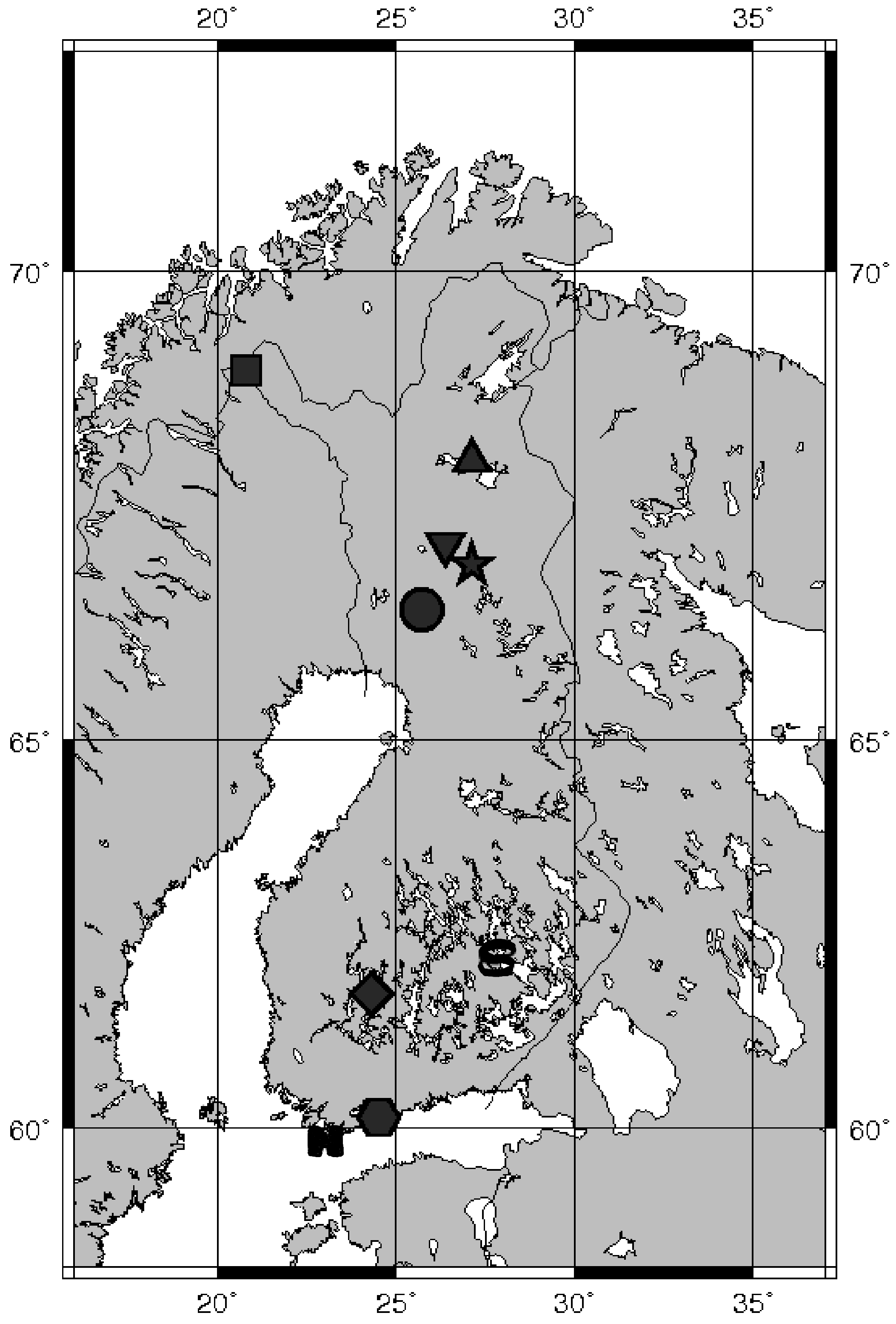
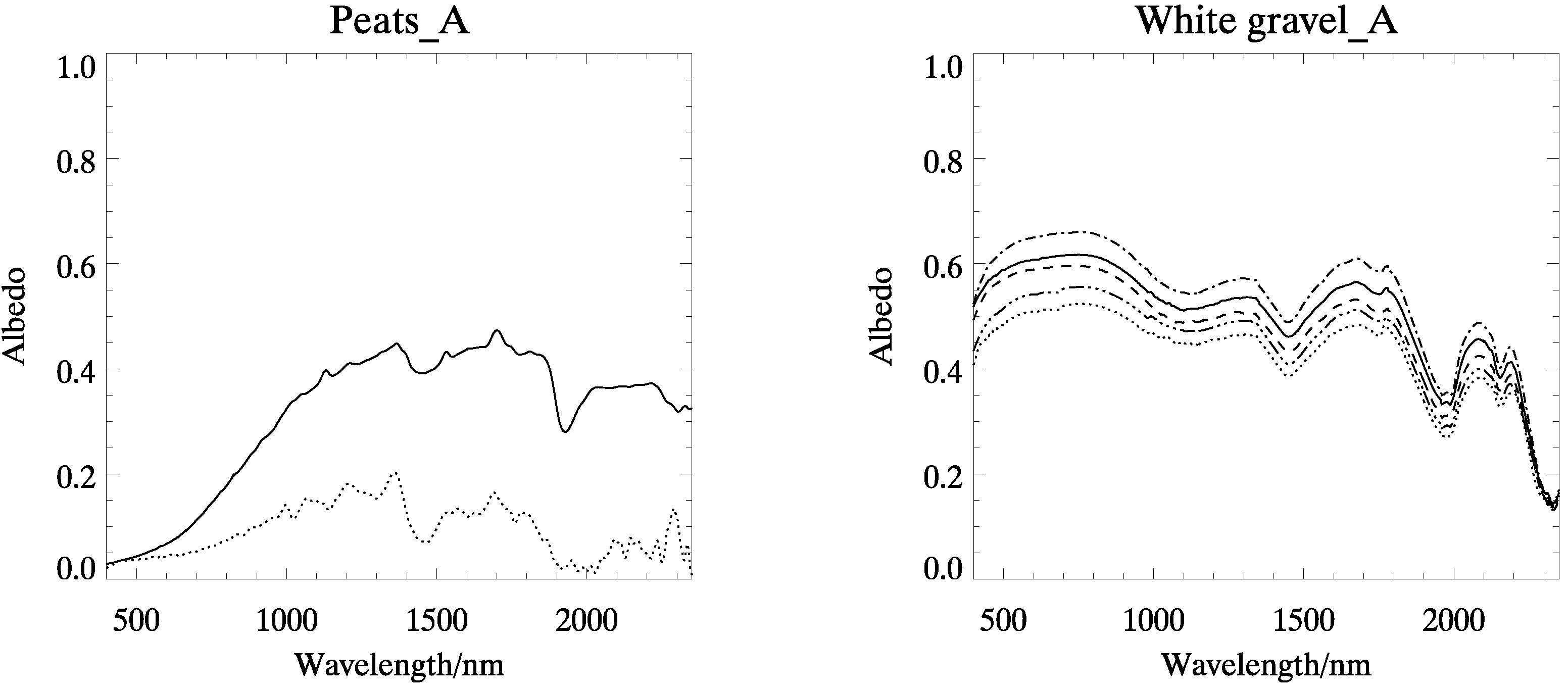
- We measured grey gravel from SjÖkulla test field [21] in a laboratory and in the field with five illumination angles. The gravel was artificially made, homogeneous, and rough, with an average grain size of 1 cm.
- We took dry sand from several locations in Finland and measured it at several illumination angles.
- 27.8.2004, Hanko beach, laboratory
- 13.9.2005, Hietalahti beach, Helsinki, sunlight
- 13.9.2005, Football field, Helsinki, sunlight
- 17.7.2006, Hietalahti beach, Helsinki, sunlight
- 8.8.2006, Sodankylä, sunlight
- 31.5.2009, beach volley field, Hyytiälä, sunlight
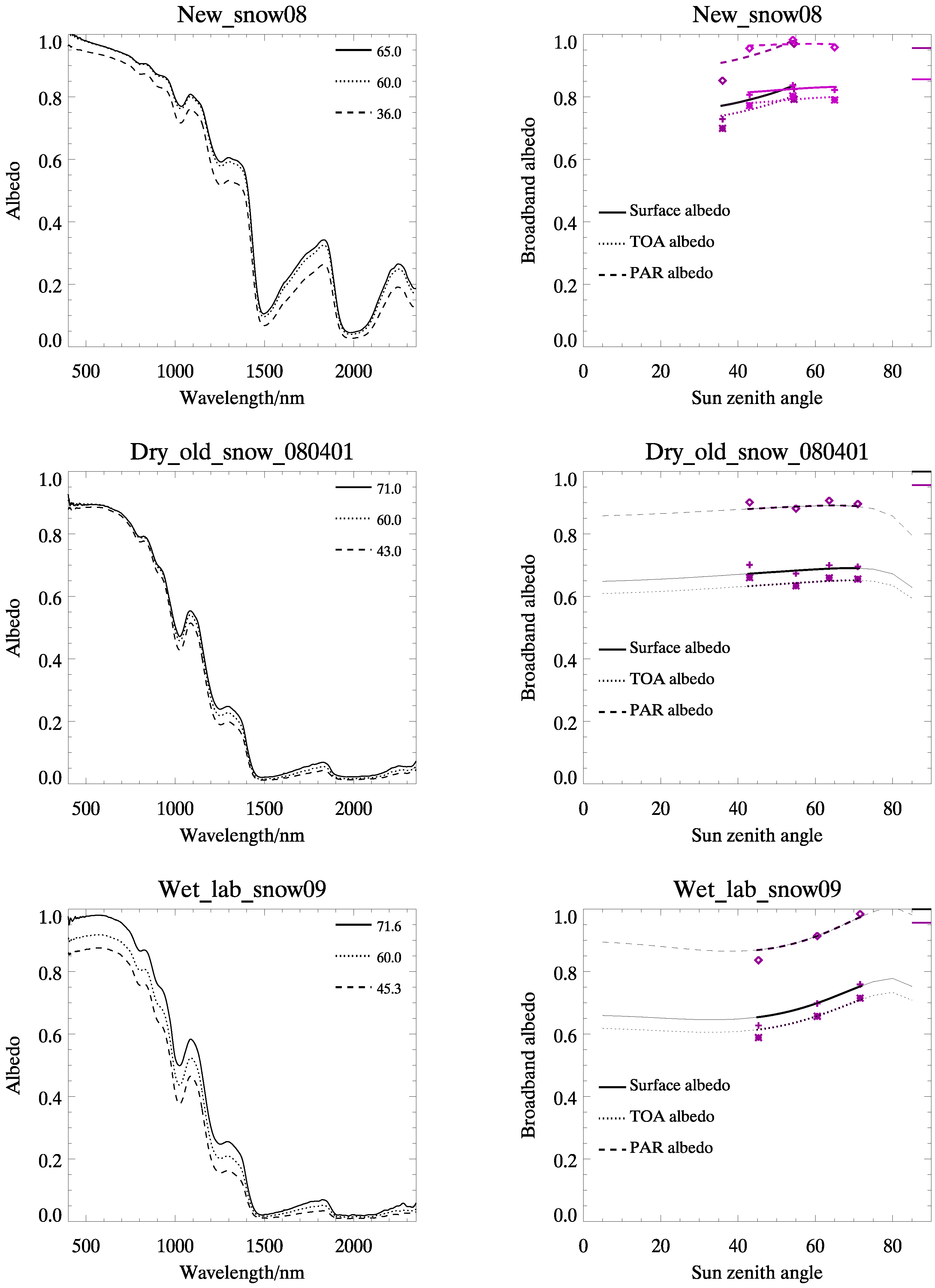
- We measured new snow in Sodankylä on two successive nights on 4–5 of March 2008 using a lamp immediately after a snow fall at five angles of illumination. The snow grains still had clear flake shapes, but they had already begun breaking up into needles.
- We measured dry old snow on 1 April 2008 in Sodankylä using a lamp at four different illumination angles. The snow was several days or weeks old, the grains were rounded, and its temperature was well below zero.
- We measured very wet melting snow in March 2009 in a laboratory in Masala using a lamp at three different illumination angles.
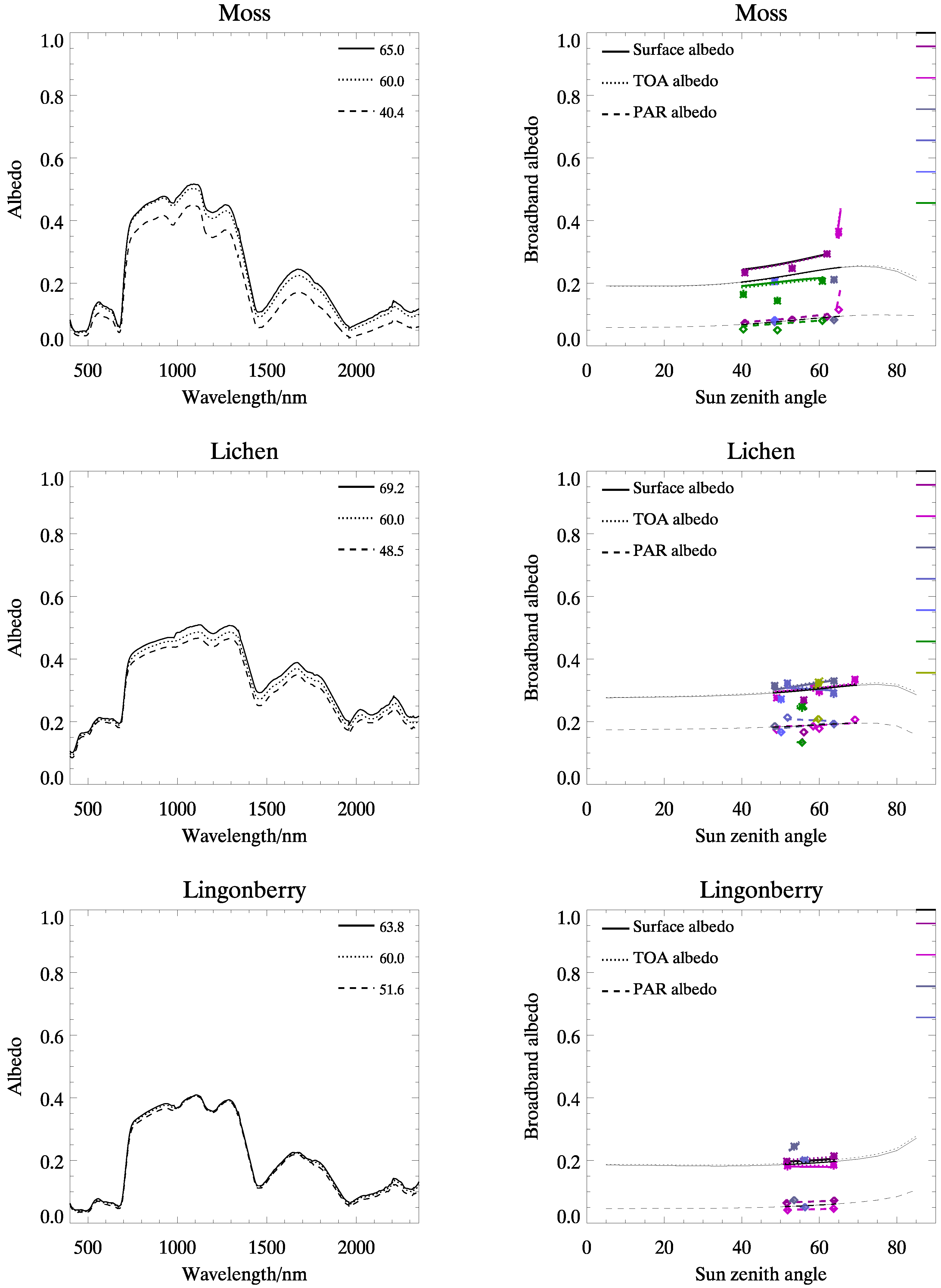
- We combined the data on Moss from measurements in Masala and Suonenjoki, both in sunlight and using a lamp, with a total of eight angles of illumination. The samples mostly consisted of Hylocomium splendens species.
- 23.8.2004, Masala, laboratory
- 24.8.2004, Masala, sunlight
- 7.6.2005, Suonenjoki, laboratory
- 7.6.2005, Suonenjoki, laboratory
- 7.6.2005, Suonenjoki, laboratory
- 2.9.2004, Masala, laboratory, Pleurozium schreberi
- We measured lichen in Suonenjoki, Sodankylä, and Masala. There were seven samples with nine angles of illumination.
- 11.7.2001, Masala, laboratory
- 18.8. 2004, Masala, laboratory
- 7.6.2005, Suonenjoki, laboratory
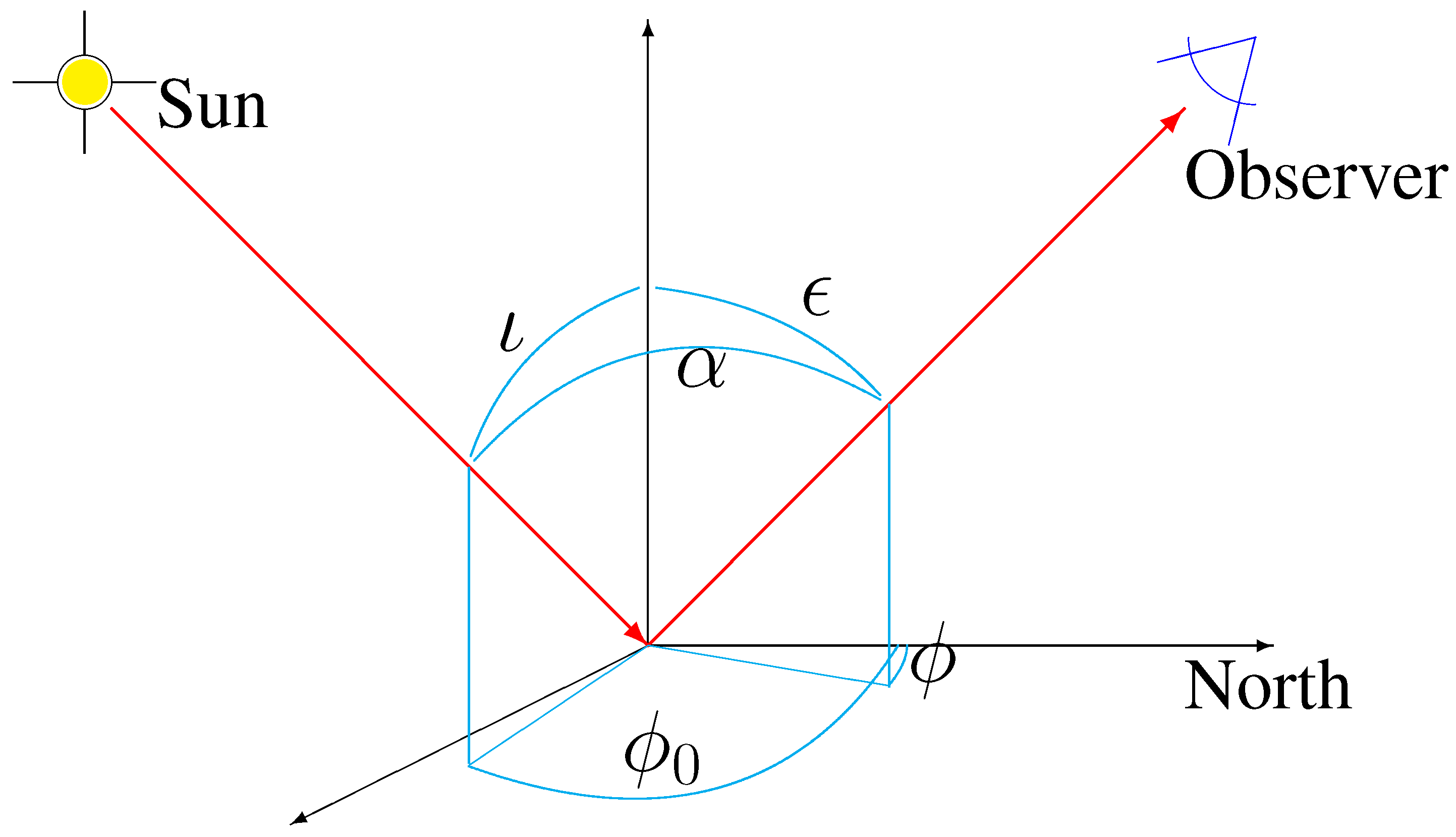
- 9.6.2005, Suonenjoki, laboratoryFigure 2. Definition of the angles used in surface reflectance work: ϵ and ι are the zenith angles of the emergent (Observer) and incident (solar) radiation respectively, φ and are the corresponding azimuths. The phase or back scattering angle α is the angle between the Observer and the Sun. The principal plane is fixed by the solar direction and the surface normal to it, while the cross plane is a vertical plane perpendicular to the principal plane.Figure 2. Definition of the angles used in surface reflectance work: ϵ and ι are the zenith angles of the emergent (Observer) and incident (solar) radiation respectively, φ and are the corresponding azimuths. The phase or back scattering angle α is the angle between the Observer and the Sun. The principal plane is fixed by the solar direction and the surface normal to it, while the cross plane is a vertical plane perpendicular to the principal plane.
![Remotesensing 02 01918 g002]()
- 3.8.2006, Sodankylä, sunlight
- 3.8.2006, Sodankylä, sunlight
- 6.8.2006, Sodankylä, sunlight
- The Lingonberry data set contained two measurements from Suonenjoki and Sodankylä.
- 8.6.2005, Suonenjoki, laboratory
- 9.6.2005, Suonenjoki, laboratory
- 5.8.2006, Sodankylä, sunlight
- 6.8.2006, Sodankylä, sunlight
- We measured an incomplete set of wet and dry peat at Suonenjoki in August 2003.


3. Results
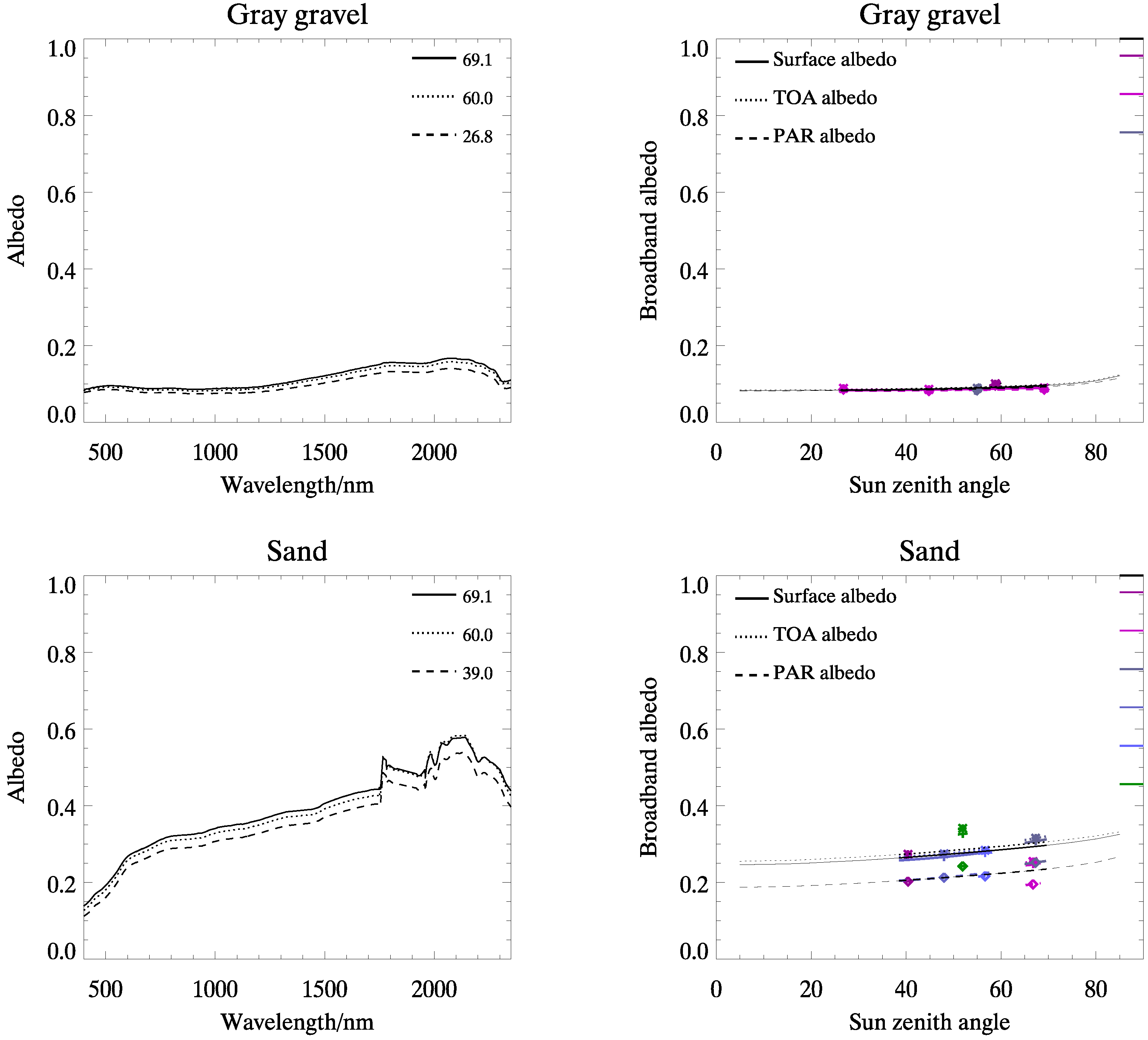
3.1. Albedos


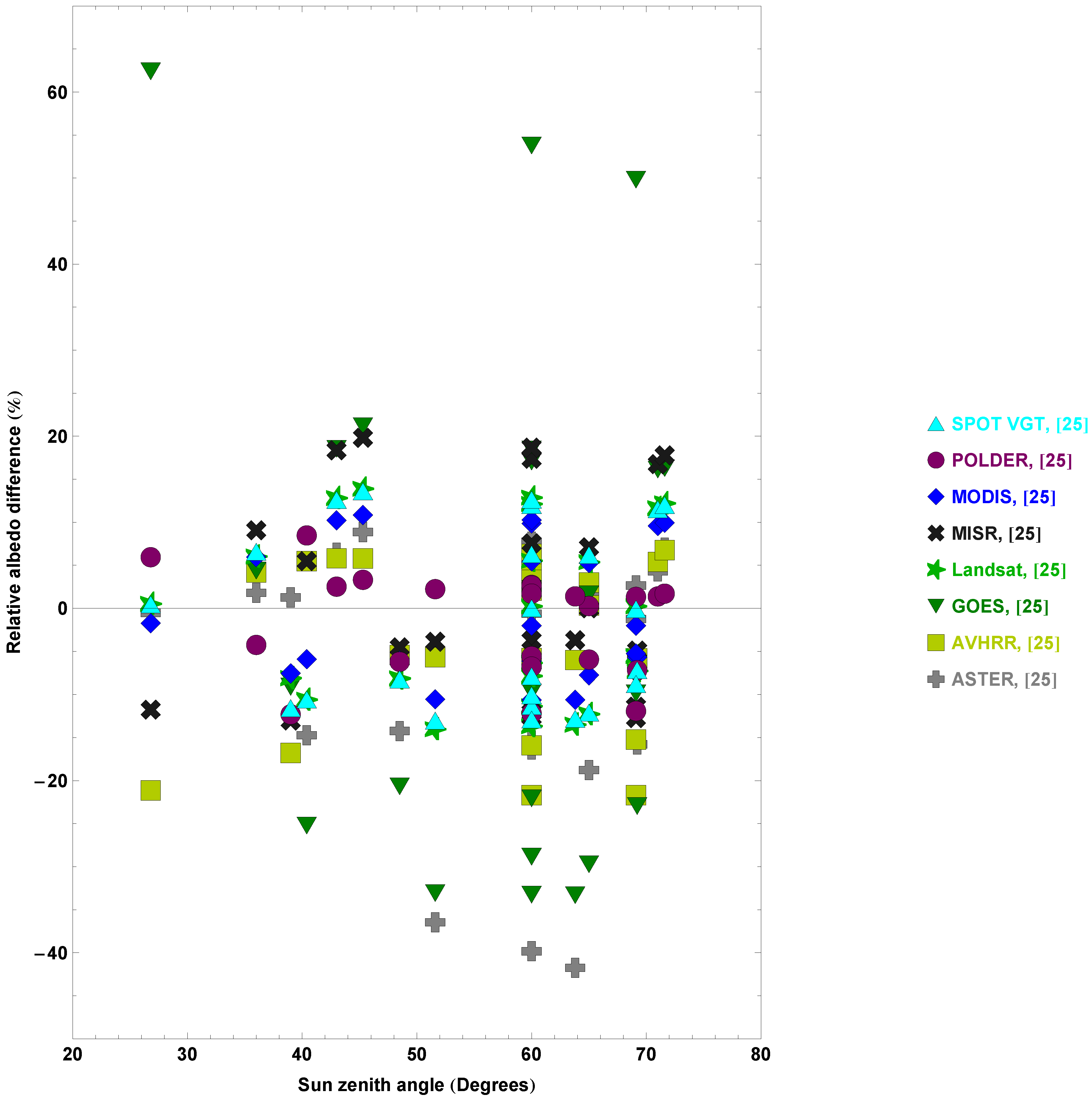
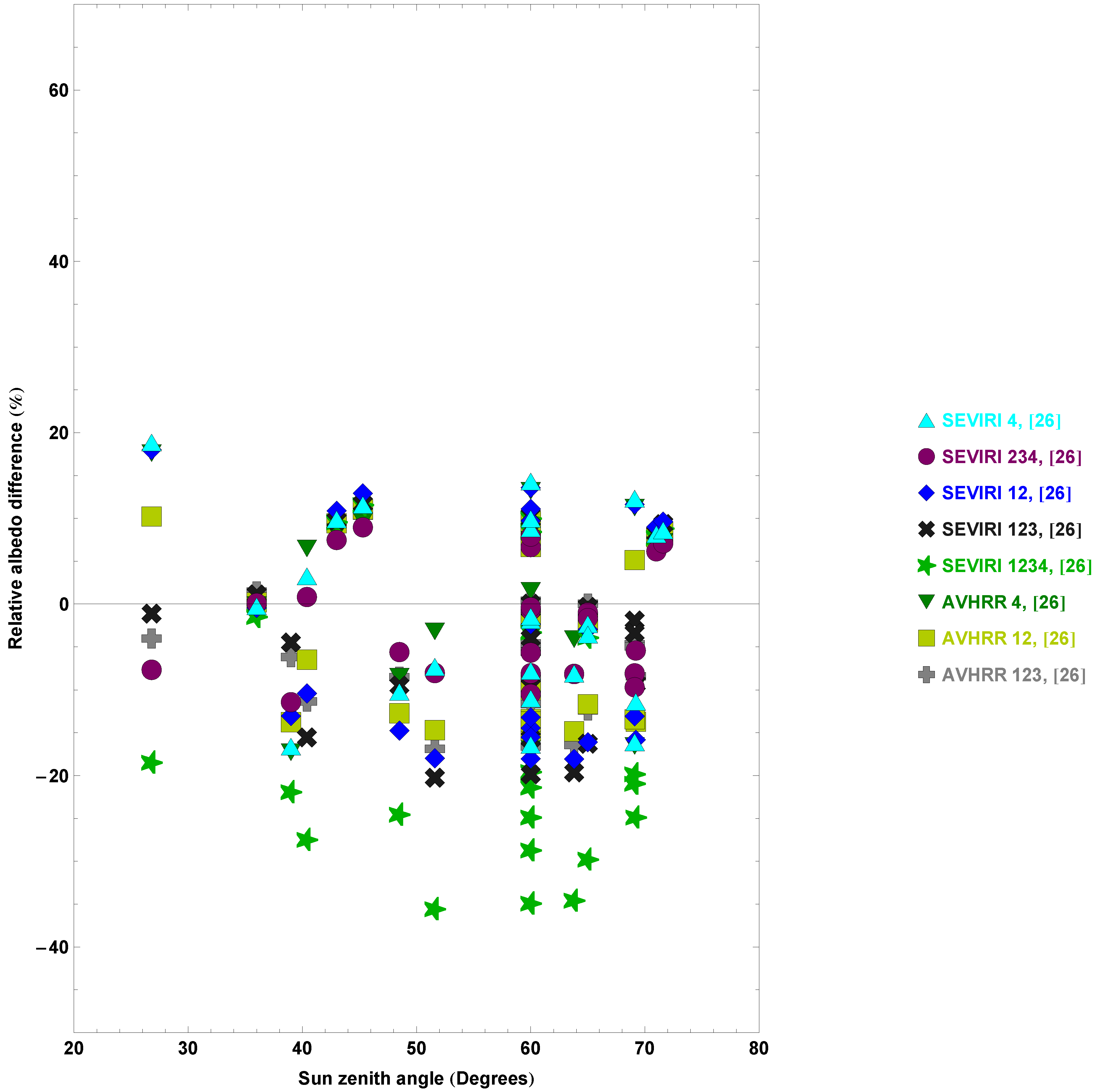
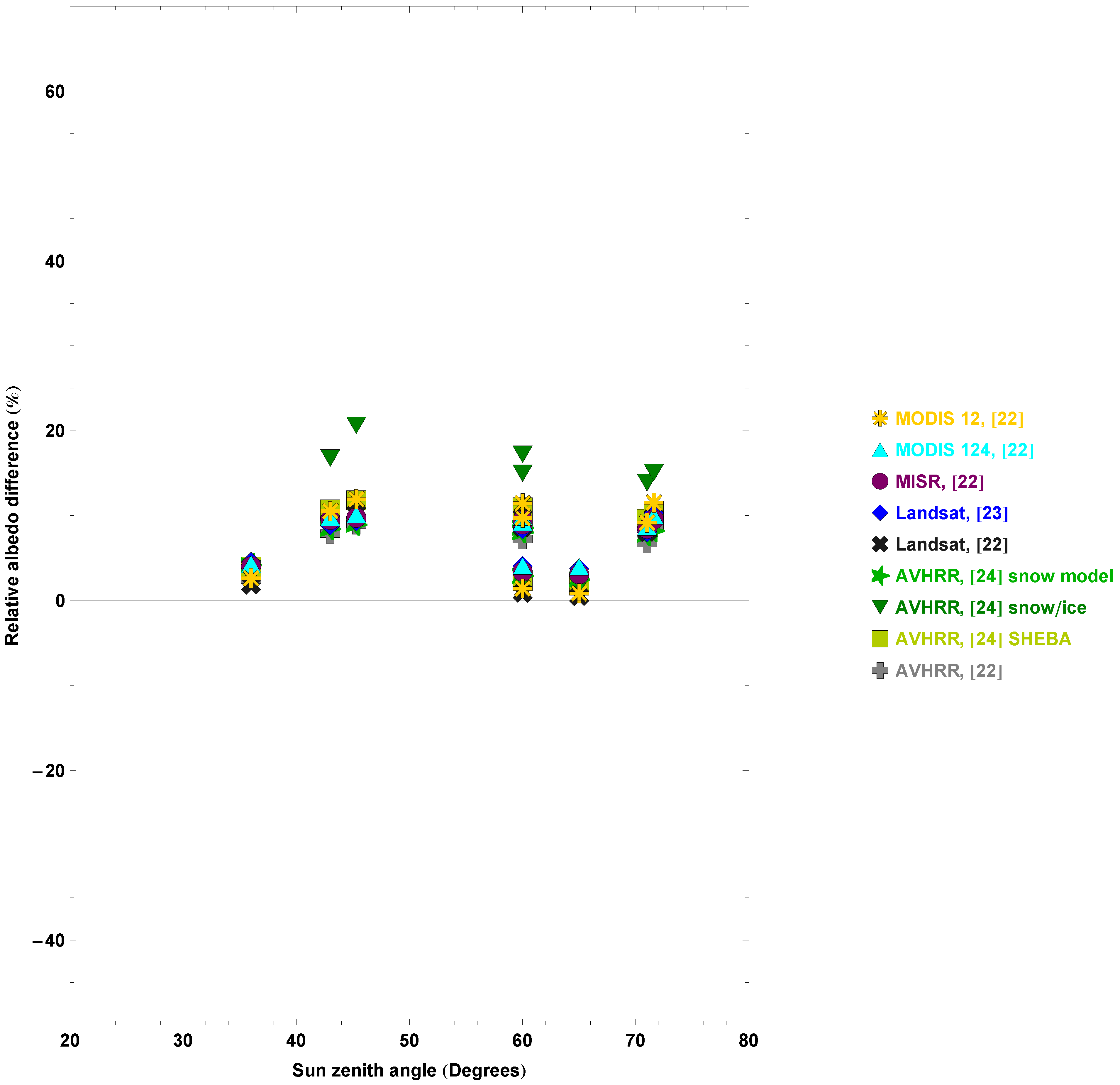
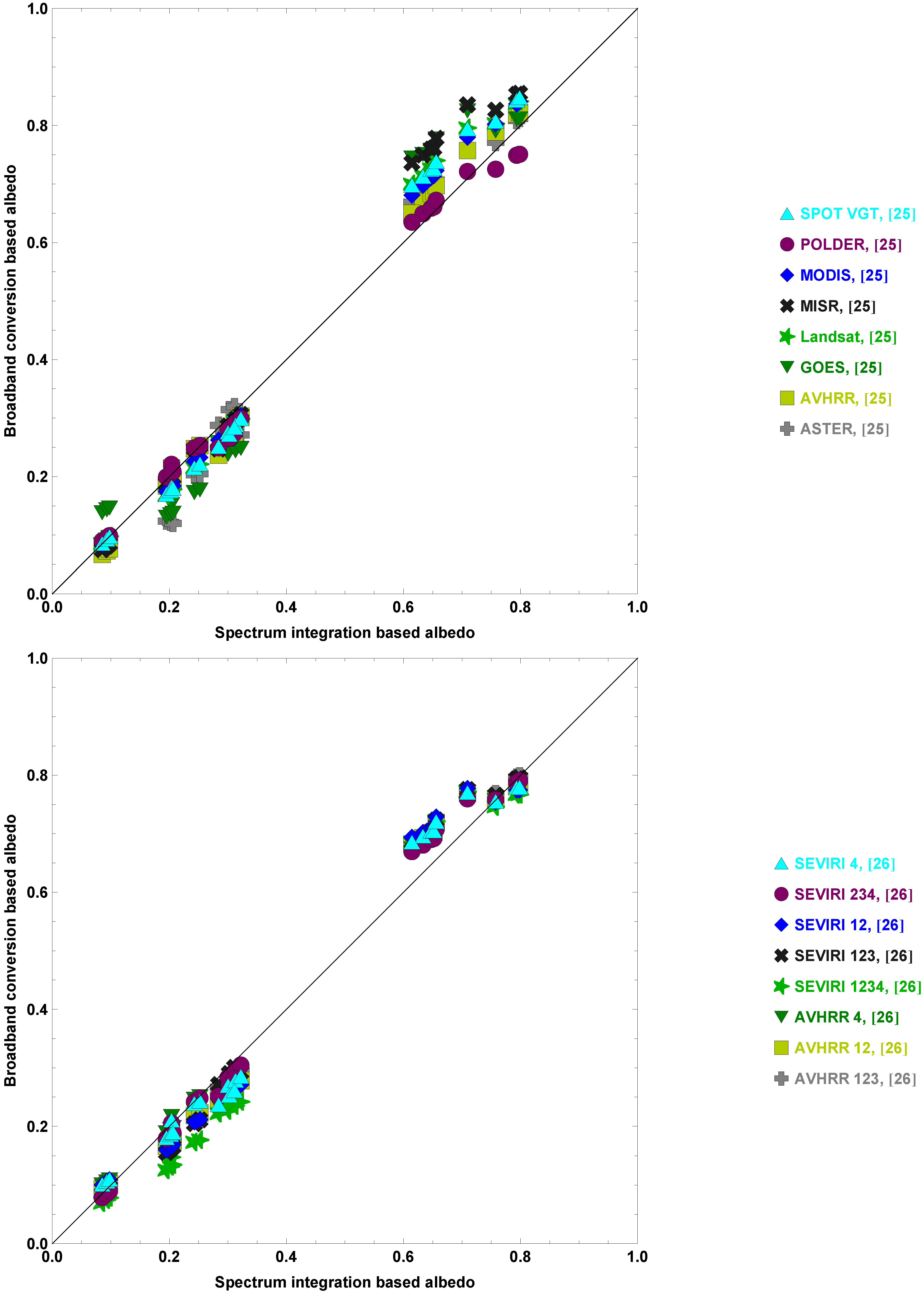
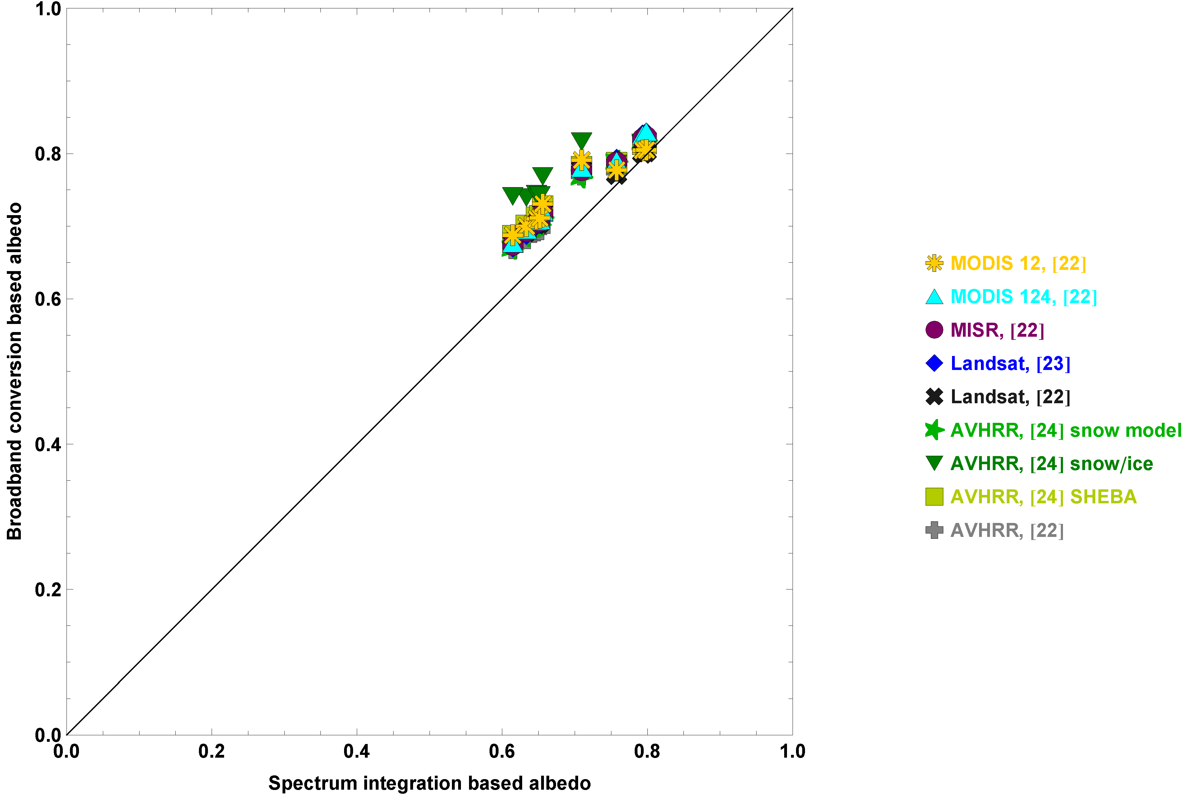
3.2. Evaluation of Narrow-to-Broadband Surface Albedo Conversion Equations


| Target | Albedo |
| Grey gravel | 0.09 |
| Lingonberry | 0.20 |
| Moss | 0.24 |
| Sand | 0.30 |
| Lichen | 0.31 |
| Dry old snow | 0.65 |
| Wet lab snow | 0.66 |
| New snow | 0.79 |


| All | Land | Snow | ||||
| Mean | Standard dev. | Mean | Standard dev. | Mean | Standard dev. | Method |
| 0.018 | 0.014 | 0.014 | 0.014 | 0.023 | 0.015 | POLDER, [25] |
| 0.022 | 0.018 | 0.015 | 0.01 | 0.034 | 0.022 | SEVIRI 234, [26] |
| 0.026 | 0.014 | 0.021 | 0.015 | 0.035 | 0.007 | AVHRR, [25] |
| 0.027 | 0.021 | 0.021 | 0.018 | 0.038 | 0.022 | AVHRR 4, [26] |
| 0.028 | 0.02 | 0.022 | 0.011 | 0.039 | 0.026 | AVHRR 123, [26] |
| 0.031 | 0.023 | 0.015 | 0.007 | 0.058 | 0.011 | MODIS, [25] |
| 0.031 | 0.024 | 0.024 | 0.016 | 0.043 | 0.03 | SEVIRI 123, [26] |
| 0.032 | 0.022 | 0.024 | 0.016 | 0.045 | 0.026 | SEVIRI 4, [26] |
| 0.034 | 0.02 | 0.028 | 0.014 | 0.043 | 0.025 | AVHRR 12, [26] |
| 0.034 | 0.025 | 0.035 | 0.03 | 0.033 | 0.017 | ASTER, [25] |
| 0.038 | 0.028 | 0.02 | 0.011 | 0.069 | 0.019 | Landsat, [25] |
| 0.04 | 0.021 | 0.034 | 0.013 | 0.051 | 0.028 | SEVIRI 12, [26] |
| 0.04 | 0.027 | 0.021 | 0.011 | 0.07 | 0.016 | SPOT VGT, [25] |
| 0.047 | 0.046 | 0.015 | 0.012 | 0.099 | 0.029 | MISR, [25] |
| 0.055 | 0.022 | 0.059 | 0.022 | 0.048 | 0.02 | SEVIRI 1234, [26] |
| 0.067 | 0.034 | 0.056 | 0.017 | 0.085 | 0.048 | GOES, [25] |
| 0.039 | 0.02 | AVHRR, [22] | ||||
| 0.043 | 0.027 | Landsat, [22] | ||||
| 0.044 | 0.015 | AVHRR, [24] snow model | ||||
| 0.049 | 0.017 | MISR, [22] | ||||
| 0.05 | 0.015 | Landsat, [23] | ||||
| 0.051 | 0.03 | MODIS 12, [22] | ||||
| 0.052 | 0.016 | MODIS 124, [22] | ||||
| 0.053 | 0.024 | AVHRR, [24] SHEBA | ||||
| 0.078 | 0.045 | AVHRR, [24] snow/ice | ||||
| Optimal/Original | Method |
| 0.03 | MODIS, [25] |
| 0.05 | Landsat, [25] |
| 0.07 | SPOT VGT, [25] |
| 0.08 | ASTER, [25] |
| 0.11 | SEVIRI 1234, [26] |
| 0.19 | AVHRR, [25] |
| 0.31 | AVHRR 123, [26] |
| 0.31 | MISR, [25] |
| 0.31 | POLDER, [25] |
| 0.35 | SEVIRI 123, [26] |
| 0.41 | SEVIRI 234, [26] |
| 0.63 | SEVIRI 12, [26] |
| 0.64 | AVHRR 12, [26] |
| 0.64 | GOES, [25] |
| 0.88 | SEVIRI 4, [26] |
| 0.95 | AVHRR 4, [26] |
4. Discussion
5. Conclusions
Author Contribution
Acknowledgements
A. Appendix
| Instrument/Resolution/ | Conversion formula, | Wavelength range of channels used in the conversion formula [μm] | ||||||
| Method | Channel 1 | Channel 2 | Channel 3 | Channel 4 | Channel 5 | Channel 6 | * | |
| ASTER, 15 m [25] | 0.52…0.6 | 0.63…0.69 | 0.78…0.86 | 1.6…1.7 | 2.15…2.18 | 2.18…2.22 | a | |
| AVHRR, 1.1 km [25] | 0.57…0.71 | 0.72…1.01 | ||||||
| GOES, 4 km [25] | 0.52…0.72 | |||||||
| Landsat, 30 km [25] | 0.45…0.51 | 0.52…0.60 | 0.63…0.69 | 0.75…0.90 | 1.55…1.75 | 2.09…2.35 | ||
| MISR, 275 m [25] | 0.42…0.45 | 0.54…0.55 | 0.66…0.67 | 0.85…0.87 | ||||
| MODIS, 500 m [25] | 0.62…0.67 | 0.84…0.87 | 0.46…0.48 | 0.54…0.56 | 1.23…1.25 | 1.63…1.65 | b | |
| POLDER, 6 km [25] | 0.43…0.46 | 0.66…0.68 | 0.74…0.79 | 0.84…0.88 | ||||
| SPOT, 1 km [25] | 0.43…0.47 | 0.61…0.68 | 0.78…0.89 | 1.58…1.75 | ||||
| EPS/AVHRR, 1 km[26] | 0.586…0.679 | 0.733…0.979 | 1.585…1.631 | 0.437…0.970 | ||||
| 123 | ||||||||
| 12 | ||||||||
| 4 | ||||||||
| SEVIRI, 5 km [26] | 0.601…0.678 | 0.780…0.839 | 1.572…1.698 | 0.476…0.910 | ||||
| 124 | ||||||||
| 123 | ||||||||
| 12 | ||||||||
| 234 | ||||||||
| 4 | ||||||||
| AVHRR, 1.1 km [22] | 0.574…0.704 | 0.720…1.000 | ||||||
| Landsat, 30 m [22] | 0.519…0.611 | 0.772…0.898 | ||||||
| MISR , 275 m [22] | 0.548…0.565 | 0.663…0.679 | 0.852…0.879 | |||||
| MODIS, [22] | 0.620…0.677 | 0.838…0.875 | 0.544…0.564 | |||||
| 500 m, 124 | ||||||||
| 250 m, 12 | ||||||||
| Landsat, 30 m [23] | 0.52…0.60 | 0.75…0.90 | ||||||
| AVHRR, 1.1 km [24] | ||||||||
| SHEBA data | 0.58…0.68 | 0.725…1.1 | ||||||
| Snow model | ||||||||
| Snow/ ice | , | |||||||
| where | ||||||||
References
- Jin, Y.; Schaaf, C.B.; Woodcock, C.E.; Gao, F.; Li, X.; Strahler, A.H.; Lucht, W.; Liang, S. Consistency of MODIS surface bidirectional reflectance distribution function and albedo retrievals: 2. Validation. J. Geophys. Res. 2003, 108. [Google Scholar] [CrossRef]
- Liang, X.Z.; Xu, M.; Gao, W.; Kunkel, K.; Slusser, J.; Dai, Y.; Min, Q.; Houser, P.R.; Rodell, M.; Schaaf, C.B.; Gao, F. Development of land surface albedo parameterization based on Moderate Resolution Imaging Spectroradiometer (MODIS) data. J. Geophys. Res. 2005, 110. [Google Scholar] [CrossRef]
- Wang, Z.; Zeng, X.; Barlage, M. Moderate Resolution Imaging Spectroradiometer bidirectional reflectance distribution function-based albedo parameterization for weather and climate models. J. Geophys. Res. 2007, 112. [Google Scholar] [CrossRef]
- Pinty, B.; Roveda, F.; Verstraete, M.; Gobron, N.; Govaerts, Y.; Martonchik, J.; Diner, D.; Kahn, R. Surface albedo retrieval from METEOSAT: Part 1. theory. J. Geophys. Res. 2000, D-105, 18099–18112. [Google Scholar] [CrossRef]
- Aminou, D. MSG’s SEVIRI Instrument. ESA Bulletin 2002, 0376–4265. [Google Scholar]
- Schulz, J.; Albert, P.; Behr, H.D.; Caprion, D.; Deneke, H.; Dewitte, S.; Dürr, B.; Fuchs, P.; Gratzki, A.; Hechler, P.; Hollmann, R.; Johnston, S.; Karlsson, K.G.; Manninen, T.; Müller, R.; Reuter, M.; Riihelä, A.; Roebeling, R.; Selbach, N.; Tetzlaff, A.; Thomas, W.; Werscheck, M.; Wolters, E.; Zelenka, A. Operational climate monitoring from space: The EUMETSAT satellite application facility on climate monitoring (CM-SAF). Atmos. Chem. Phys. 2009, 9, 1–23. [Google Scholar] [CrossRef]
- Diner, D.J.; Braswell, B.; Davies, R.; Gobron, N.; Hu, J.; Jin, Y.; Kahn, R.; Knyazikhin, Y.; Loeb, N.; Muller, J.P.; Nolin, A.; Pinty, B.; Schaaf, C.; Seiz, G.; Stroeve, J. The value of multiangle measurements for retrieving structurally and radiatively consistent properties of clouds, aerosols, and surfaces. Remote Sens. Environ. 2005, 97, 495–518. [Google Scholar] [CrossRef]
- Pirazzini, R. Surface albedo measurements over Antarctic sites in summer. J. Geophys. Res. 2004, 109. [Google Scholar] [CrossRef]
- Pirazzini, R. Factors Controlling the Surface Energy Budget over Snow and Ice. Ph.D. Thesis, Department of Physics, University of Helsinki, Helsinki, Finland, 2008. [Google Scholar]
- Riihelä, A.; Manninen, T. Measuring the vertical albedo profile of a subarctic boreal forest canopy. Silva Fennica 2008, 42, 807–815. [Google Scholar] [CrossRef]
- Manninen, T.; Riihelä, A. Atmospheric effect on validation of broadband surface albedo (SAL) product of CM SAF using mast measurements. In Proceedings of the EUMETSAT Meteorological Satellite Conference, Darmstadt, Germany, 2008.
- Manninen, T.; Stenberg, P. Simulation of the effect of snow covered forest floor on the total forest albedo. Agr. Forest Meteoro. 2008, 149, 303–319. [Google Scholar] [CrossRef]
- Manninen, T.; Siljamo, N.; Poutiainen, J. Validation of the surface albedo product (SAL) of CM SAF in winter conditions. In Proceedings of the EUMETSAT Meteorological Satellite Conference, Maputo, Mozambique, 2006; pp. 48–54.
- Peltoniemi, J.; Kaasalainen, S.; Näränen, J.; Rautiainen, M.; Stenberg, P.; Smolander, H.; Smolander, S.; Voipio, P. BRDF measurement of understory vegetation in pine forests: dwarf shrubs, lichen and moss. Remote Sens. Environ. 2005, 94, 343–354. [Google Scholar] [CrossRef]
- Peltoniemi, J.; Kaasalainen, S.; Näränen, J.; Matikainen, L.; Piironen, J. Measurement of directional and spectral signatures of light reflectance by snow. IEEE Trans. Geosci. Remote Sens. 2005, 43, 2294–2304. [Google Scholar] [CrossRef]
- Peltoniemi, J.; Piironen, J.; Näränen, J.; Suomalainen, J.; Kuittinen, R.; Honkavaara, E.; Markelin, L. Bidirectional reflectance spectrometry of gravel at the Sjökulla test field. ISPRS J. Photogramm. Remote Sens. 2007, 62, 434–446. [Google Scholar] [CrossRef]
- Puttonen, E.; Suomalainen, J.; Hakala, T.; Peltoniemi, J. Measurement of reflectance properties of asphalt surfaces and their usability as reference targets for aerial photos. IEEE Trans. Geosci. Remote Sens. 2009, 47, 2330–2339. [Google Scholar] [CrossRef]
- Suomalainen, J.; Hakala, T.; Puttonen, E.; Peltoniemi, J. Polarised bidirectional reflectance factor measurements from vegetated land surfaces. J. Quant. Spectrosc. Radiat. Transfer 2009, 110, 1044–1056. [Google Scholar] [CrossRef]
- Peltoniemi, J.; Hakala, T.; Suomalainen, J.; Puttonen, E. Polarised bidirectional reflectance factor measurements from snow, soil and gravel. J. Quant. Spectrosc. Radiat. Transfer 2009, 110, 1940–1953. [Google Scholar] [CrossRef]
- Suomalainen, J.; Hakala, T.; Peltoniemi, J.; Puttonen, E. Polarised Multiangular Reflectance Measurements Using Finnish Geodetic Institute Field Goniospectrometer. Sensors 2009, 9, 3891–3907. [Google Scholar] [CrossRef] [PubMed]
- Honkavaara, E.; Peltoniemi, J.; Ahokas, E.; Kuittinen, R.; Hyyppä, J.; Jaakkola, J.; Kaartinen, H.; Markelin, L.; Nurminen, K.; Suomalainen, J. A permanent test field for digital photogrammetric systems. Photogramm. Eng. Remote Sens. 2008, 74, 95–106. [Google Scholar] [CrossRef]
- Greuell, W.; Oerlemans, J. Narrowband-to-broadband albedo conversion for glacier ice and snow: equations based on modeling and ranges of validity of the equations. Remote Sens. Environ. 2004, 89, 95–105. [Google Scholar] [CrossRef]
- Knap, W.; Oerlemans, J. The surface albedo of the Greenland ice sheet: Satellite-derived and in situ measurements in the Søndre Strøfjord area during the 1991 melt season. J. Glaciol. 1996, 42, 364–374. [Google Scholar]
- Xiong, X.; Stamnes, K.; Lubin, D. Surface Albedo over the Arctic Ocean Derived from AVHRR and Its Validation with SHEBA Data. J. Appl. Meteor. 2002, 41, 413–425. [Google Scholar] [CrossRef]
- Liang, S. Narrowband to broadband conversions of land surface albedo. I Algorithms. Remote Sens. Environ. 2000, 76, 213–238. [Google Scholar] [CrossRef]
- van Leeuwen, W.; Roujean, J.L. Land surface albedo from the synergistic use of polar (EPS) and geo-stationary (MSG) observing systems. An assessment of physical uncertainties. Remote Sens. Environ. 2002, 81, 273–289. [Google Scholar] [CrossRef]
- Privette, J.L.; Eck, T.F.; Deering, D.W. Estimating spectral albedo and nadir reflectance through inversion of simple BRDF models with AVItRR/MODIS-Iike. J. Geophys. Res. 1997, 102, 29529–29542. [Google Scholar] [CrossRef]
- Wang, Z.; Barlage, M.; Zeng, X.; Dickinson, R.E.; Schaaf, C.B. The solar zenith angle dependence of desert albedo. Geophys. Res. Lett. 2005, 32. [Google Scholar] [CrossRef]
- Grenfell, T.; Warren, S.; Mullen, P. Reflection of solar radiation by the Antarctic snow surface at ultraviolet, visible and near-infrared wavelengths. J. Geophys. Res. 1994, 99, 18669–18684. [Google Scholar] [CrossRef]
- Wuttke, S.; Seckmeyer, G.; König-Langlo, G. Measurements of spectral snow albedo at Neumayer, Antarctica. Ann. Geophys. 2006, 24, 7–21. [Google Scholar] [CrossRef] [Green Version]
- Song, J. Diurnal asymmetry in surface albedo. Agr. Forest Meteor. 1998, 92, 181–189. [Google Scholar] [CrossRef]
© 2010 by the authors; licensee MDPI, Basel, Switzerland. This article is an open access article distributed under the terms and conditions of the Creative Commons Attribution license (http://creativecommons.org/licenses/by/3.0/).
Share and Cite
Peltoniemi, J.I.; Manninen, T.; Suomalainen, J.; Hakala, T.; Puttonen, E.; Riihelä, A. Land Surface Albedos Computed from BRF Measurements with a Study of Conversion Formulae. Remote Sens. 2010, 2, 1918-1940. https://doi.org/10.3390/rs2081918
Peltoniemi JI, Manninen T, Suomalainen J, Hakala T, Puttonen E, Riihelä A. Land Surface Albedos Computed from BRF Measurements with a Study of Conversion Formulae. Remote Sensing. 2010; 2(8):1918-1940. https://doi.org/10.3390/rs2081918
Chicago/Turabian StylePeltoniemi, Jouni I., Terhikki Manninen, Juha Suomalainen, Teemu Hakala, Eetu Puttonen, and Aku Riihelä. 2010. "Land Surface Albedos Computed from BRF Measurements with a Study of Conversion Formulae" Remote Sensing 2, no. 8: 1918-1940. https://doi.org/10.3390/rs2081918