Chlorophyll-a Detection Algorithms at Different Depths Using In Situ, Meteorological, and Remote Sensing Data in a Chilean Lake

Abstract

In this study, we employ in situ, meteorological, and remote sensing data to estimate chlorophyll-a concentration at different depths in a South American freshwater ecosystem, focusing specifically on a lake in southern Chile known as Lake Maihue. For our analysis, we explored four different scenarios using three deep learning and traditional statistical models. These scenarios involved using field data (Scenario 1), meteorological variables (Scenario 2), and satellite data (Scenarios 3.1 and 3.2) to predict chlorophyll-a levels in Lake Maihue at three different depths (0, 15, and 30 m). Our choice of models included SARIMAX, DGLM, and LSTM, all of which showed promising statistical performance in predicting chlorophyll-a concentrations in this lake. Validation metrics for these models indicated their effectiveness in predicting chlorophyll levels, which serve as valuable indicators of the presence of algae in the water body. The coefficient of determination values ranged from 0.30 to 0.98, with the DGLM model showing the most favorable statistics in all scenarios tested. It is worth noting that the LSTM model yielded comparatively lower metrics, mainly due to the limitations of the available training data. The models employed, which use traditional statistical and machine learning models and meteorological and remote sensing data, have great potential for application in lakes in Chile and the rest of the world with similar characteristics. In addition, these results constitute a fundamental resource for decision-makers involved in the protection and conservation of water resource quality.

1. Introduction

Remote lakes, defined as bodies of water located in geographically isolated or inaccessible areas [1], are typically found in mountainous regions, polar landscapes, tropical rainforests, or anywhere with significant natural barriers, such as steep terrain or dense vegetation [2,3]. Their defining characteristics include their remoteness from urbanized areas and limited exposure to human activity [4]. The difficult accessibility of these lakes often results in their preservation, allowing them to remain virtually untouched and to maintain their natural beauty and biodiversity [4,5,6]. Not having suffered direct human influence, these bodies of water offer pristine environments and relatively intact ecosystems [7,8]. In Chile, the Andes Mountains are home to numerous remote lakes due to the geomorphological characteristics of the country [9].

Due to their isolation and relative inaccessibility, remote lakes often become the focus of scientific studies and research aimed at understanding aquatic ecosystems and their interactions with the surrounding environment [10,11]. In addition, these lakes can play a crucial role in biodiversity conservation by acting as refuges for vulnerable or endangered species [12]. However, recent studies, including [13,14,15], have reported algal bloom episodes in mountain lakes away from humans and other settlements [14,15,16], where human influence is more pronounced.

With the development of technology and communications, remote sensing has become an alternative tool to traditional monitoring, especially in remote areas, such as lakes, where it provides valuable information on water quality parameters [17]. Chlorophyll-a is a pigment found in all aquatic and terrestrial plants and is an important indicator of water quality and the health of aquatic ecosystems [18]. Reflectance derived from bands of the electromagnetic spectrum can be obtained from multispectral images taken by various instruments aboard satellites [19,20]. Algorithms applied to these images use this information to extract relevant features from the images, such as the wavelength and intensity of reflected light, which are related to the presence of chlorophyll-a [21,22]. These features are combined with the data from the satellite and with training data from the machine learning model to create an algorithm that can detect and quantify chlorophyll-a in new images [23].

Chlorophyll-a detection algorithms using combined machine learning and remote sensing techniques are new advanced tools used to assess the presence and concentration of chlorophyll-a in water bodies [24,25,26]. Machine learning consists of training a model with previously labeled sample data, which allows the algorithm to learn to recognize patterns and make accurate predictions about chlorophyll-a concentration in new images [27,28,29]. The combination of machine learning and remote sensing techniques allows for improved accuracy of chlorophyll-a detection compared to traditional approaches [30,31,32,33]. These algorithms can be applied to different types of water bodies, such as lakes, rivers, and oceans, and are especially useful for large-scale water quality monitoring [34,35,36,37]. Accurate chlorophyll-a detection provides valuable information for water resource management, environmental impact assessments, and early detection of phenomena such as harmful algal blooms [38,39]. The objective of this work is to combine the previously described techniques of remote sensing and machine learning in a remote lake of the Andes Mountain range in Chile to predict the behavior of the variable chlorophyll-a concentrations at different depths as a bioindicator of the trophic state of this lake body. The specific objectives are as follows: (i) to collect baseline information on the behavior of limnological parameters in the period of 2001–2020; (ii) to create an estimation model of Chl-a using in situ, meteorological, and remote sensing data; and (iii) to validate the accuracy of the model with statistical metrics.

2. Materials and Methods

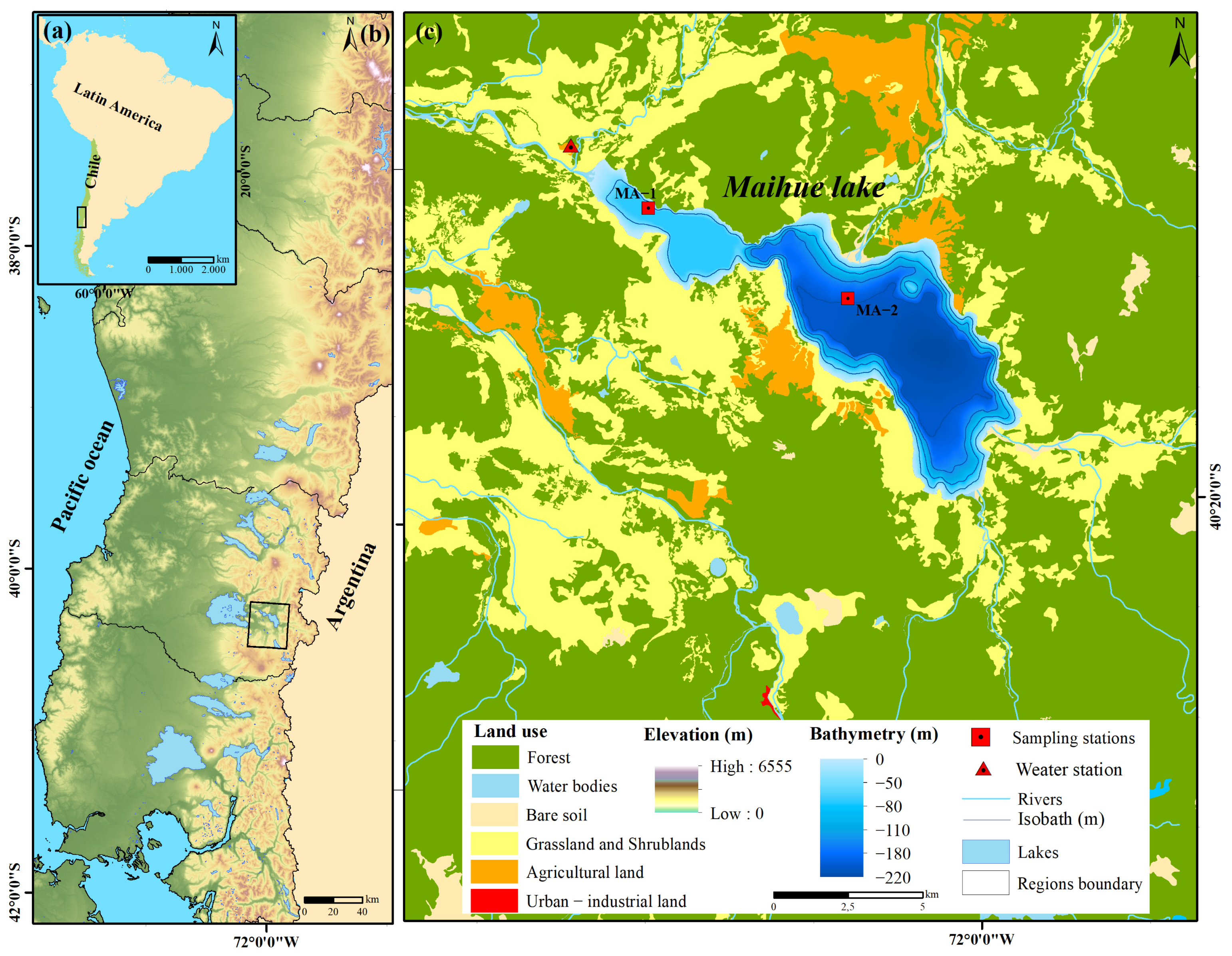
2.1. Site Description

Lake Maihue is located between 40°16′S and 72°03′W in the Los Rios region of southern Chile [40]. Maihue is an overdeepened glacigenic lake dammed by frontal moraines [41]. This lake in the Araucanian Lake District has a maximum depth of 207 m and covers an area of 47.2 km² [42]. Its waters are of an intense blue color and are fed by several rivers and streams that descend from the surrounding mountains [43]. In addition, Lake Maihue has several islands scattered across its surface, which adds visual appeal to its landscape. In terms of its geographic setting, Lake Maihue is in an area of abundant vegetation and native forests [43]. Native forests surround its shores, mainly of species such as Nothofagus dombeyi (coigüe), Eucryphia cordifolia (ulmo), and Podocarpus nubigenus (mañío). In addition, nearby you can find waterfalls, rivers, and streams that are fed by melting glaciers in the Cordillera. The climate of the Andes is extreme, with strong winds, rainfall, and high solar radiation [44]. Lake Maihue has temperatures ranging from 6.5 °C in winter to 19.5 °C in summer (DGA Chile, accessed 28 June 2023).

2.2. Sampling Measurements and Meteorological Data

The Dirección General de Aguas de Chile (DGA) monitors several lakes in the Chilean territory, including Lake Maihue. For this study, we selected the monitoring campaigns carried out in the summer and spring from 2001 to 2020. The physicochemical and biological parameters of the water included in the chlorophyll-a estimation model were Chl-a, a Secchi disk, temperature (°C), total nitrogen (NT) (mg/L), total phosphorus (mg/L), and NTU turbidity. On the other hand, some meteorological variables, such as precipitation (mm), air temperature (°C), relative humidity (%), and wind speed (m/s), were selected. Precipitation was obtained from the Lago Maihue station (Figure 1) from the Dirección General de Aguas de Chile (DGA) at https://dga.mop.gob.cl/Paginas/default.aspx and consulted on 20 September 2023. This station is the closest and most representative of the lake.

2.3. Satellite Images and Processing

The multispectral bands of the Landsat satellite have a high resolution of 30 m and cover the study period (2001–2020), which is why they were used in this research. Landsat is a project operated by the National Aeronautics and Space Administration (NASA) and the United States Geological Survey (USGS) [45], and images are available on the USGS Earth Explorer at https://earthexplorer.usgs.gov/ accessed on 20 September 2023. A total of 19 Landsat 5, 7, and 8 images (L-5, L-7, and L-8) were downloaded with a low percentage of clouds covering the study lake (path/row: 232/88 and 233/88) and corresponding to Collection 2 Level 1 (see

Table 1. Characteristics of satellite images.

N	Image Id	Path/Row	Year	In Situ Date	Image Date	Days Difference
1	LE07_L1TP_233088_20020305_20211023_02_T1	233/88	2002	06-03-2002	05-03-2002	1
2	LE07_L1TP_233088_20030324_20200915_02_T1	233/88	2003	18-03-2003	24-03-2003	6
3	LT05_L1TP_233088_20031127_20201008_02_T1	233/88	2003	17-11-2003	27-11-2003	10
4	LT05_L1TP_232088_20040311_20200903_02_T1	232/88	2004	01-03-2004	11-03-2004	10
5	LT05_L1TP_232088_20040818_20200903_02_T1	232/88	2004	20-08-2004	18-08-2004	2
6	LT05_L1TP_232088_20041122_20200902_02_T1	232/88	2004	17-11-2004	22-11-2004	5
7	LT05_L1TP_232088_20060213_20200901_02_T1	232/88	2006	09-02-2006	13-02-2006	4
8	LT05_L1TP_233088_20060527_20200901_02_T1	233/88	2006	24-05-2006	27-05-2006	3
9	LT05_L1TP_233088_20060730_20200831_02_T1	233/88	2006	12-08-2006	30-07-2006	12
10	LT05_L1TP_233088_20061103_20200831_02_T1	233/88	2006	26-10-2006	03-11-2006	7
11	LT05_L1TP_233088_20070818_20200830_02_T1	233/88	2007	19-08-2007	18-08-2007	1
12	LT05_L1TP_232088_20080219_20200829_02_T1	232/88	2008	23-02-2008	19-02-2008	4
13	LT05_L1TP_232088_20090221_20200828_02_T1	232/88	2009	17-02-2009	21-02-2009	4
14	LT05_L1TP_233088_20091111_20200825_02_T1	233/88	2009	17-11-2009	11-11-2009	6
15	LC08_L1TP_233088_20131208_20200912_02_T1	233/88	2013	03/05-12-2013	08-12-2013	3, 5
16	LC08_L1TP_233088_20140226_20200911_02_T1	233/88	2014	19-02-2014	26-02-2014	7
17	LC08_L1TP_233088_20150213_20200909_02_T1	233/88	2015	10/11-02-2015	13-02-2015	2, 3
18	LC08_L1TP_233088_20200126_20200823_02_T1	233/88	2020	26-01-2020	26-01-2020	0
19	LC08_L1TP_232088_20201118_20210315_02_T1	232/88	2020	22-11-2020	18-11-2020	4

). To mask clouds, quality assessment (QA) bands were used and analyzed by visual inspection. Only those with the lowest percentage of cloud cover over the lake and those as close as possible to the sampling dates were selected.

Images were atmospherically corrected in the ACOLITE software (version 20211124.0) at https://github.com/acolite accessed on 20 September 2023. This software contains the atmospheric correction protocols and processing developed at RBINS for aquatic remote sensing applications (llori et al., 2019). The default atmospheric correction used was the DSF algorithm approach “Dark Spectrum Fitting” [46,47,48] and the older “exponential extrapolation” or EXP algorithm [49,50,51]. From the processing, surface-level reflectance (ρs) is obtained, and the values are extracted per 3 × 3 pixel matrix [15,52]. The software used to extract the pixel values was ArcGIS (ESRI v. 10.8.2). Then, the values of the band combinations and the calculated spectral indices are also obtained. The area of interest (Roi) was established from geospatial data provided by the General Directorate of Waters of Chile (DGA), accessed on 02 March 2023.

2.4. Vegetation Indices, Band, and Band Combination

Water quality parameters, such as chlorophyll, have been estimated with great precision using satellite data in lakes [18,39,53,54]. The blue (B), green (G), red (R), near infrared (NIR), and shortwave infrared (SWIR) multispectral bands were used, as well as some combinations of bands and vegetation spectral indices (see

Table 2. Definition of the spectral indices used in this study.

Indices	Formula	Reference
Spectral bands	4 bands (B, R, G,NIR)	[18]
Floating Algal Index (Fai)	FAI = Rnir − R′nir R′nir = Rred + (Rswir − Rred) × (λnir − λred)/(λswir − λred)	[40]
Green Normalized Difference Vegetation Index (Gndvi)	(NIR − G)/(NIR + G)	[13]
Normalized Difference Vegetation Index (Ndvi)	(NIR − R)/(NIR + R)	[13]
Surface Algal Bloom Index (Sabi)	(NIR − R)/(B + G)	[15]
Green Chlorophyll Index (Gci)	GCI = (NIR/G) − 1	[13]

). The spectral bands and their combinations (N/R, R/N, and B/G) have been widely used in the literature due to their excellent results in retrieving the concentration of chlorophyll [18,39,55,56]. Furthermore, spectral indices derived from the above-mentioned bands are currently the most used ones for monitoring the concentration of chlorophyll [14,39,57,58]. The normalized difference vegetation index (NDVI), obtained as the ratio between the NIR and R reflectances and their sum, is an indicator of photosynthetic activity and changes in vegetation [59,60]. The surface algal bloom index (SABI), obtained as the ratio between the NIR and R reflectances and the sum of the B and G reflectances, is an index proposed to delineate the spatial distributions of floating algae or emergent vegetation extraction in aquatic systems [15,61]. The floating algal index (FAI) is an indicator capable of detecting floating algae in different aquatic environments and is a very efficient index for the detection of surface vegetation related to chlorophyll. It is obtained from the relationships between the NIR, R, and SWIR bands [62,63]. The green normalized difference vegetation index (GNDVI) is resistant to atmospheric effects and very sensitive to chlorophyll-a concentrations. It is calculated from the NIR and G bands [55,64]. The last index calculated was the green chlorophyll index (GCI) [65,66]. This can be used to estimate the chlorophyll content of leaves and has been used to detect chlorophyll and algal blooms in some research. It uses NIR and G wavelengths [15].

2.5. Prediction Using Statistical and Machine Learning Models

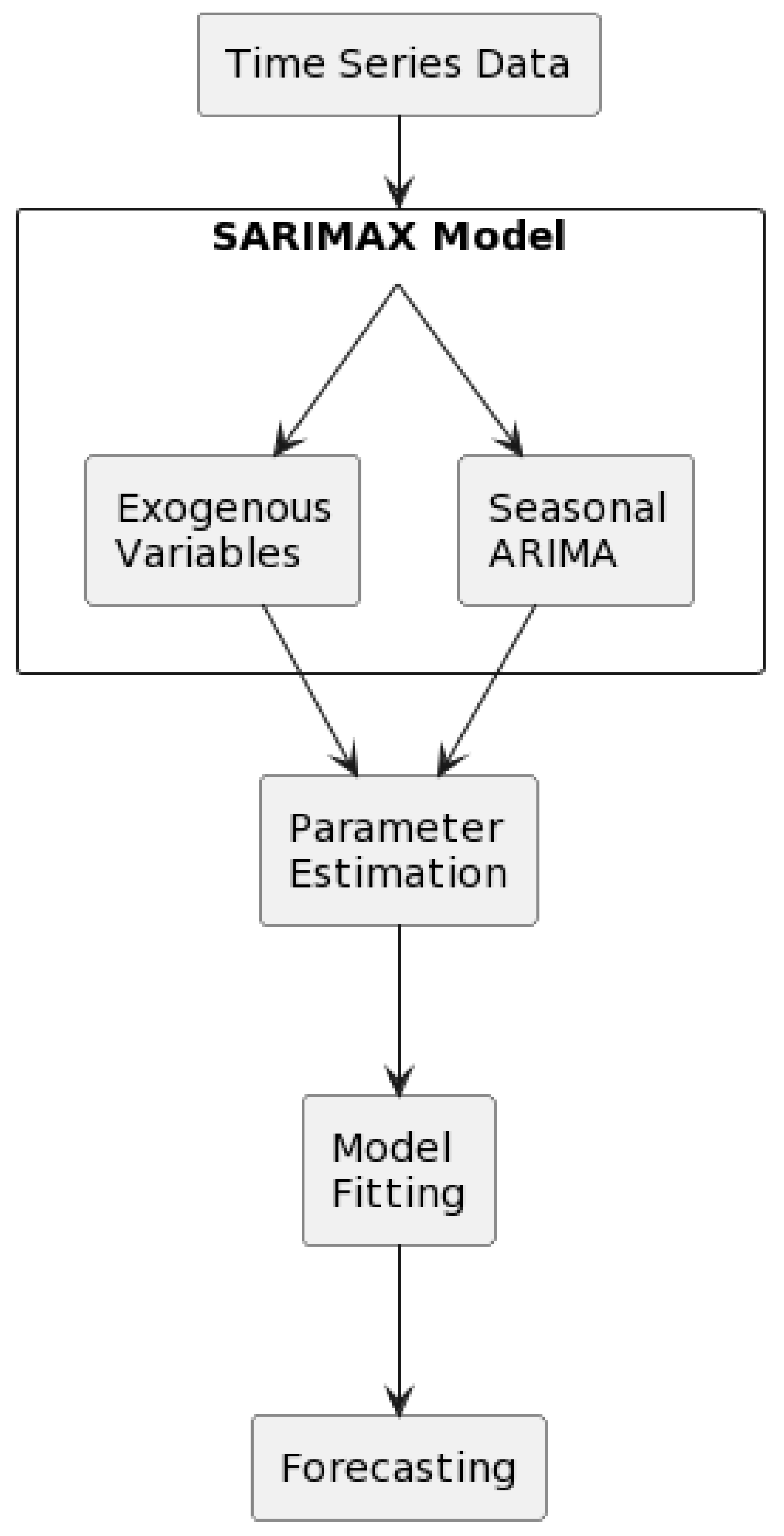
2.5.1. SARIMAX

The SARIMAX (seasonal autoregressive integrated moving average with exogenous regressors) model is an extension of the SARIMA (seasonal autoregressive integrated moving average) model that allows for the inclusion of exogenous variables in time series modeling (see Figure 2). SARIMA models are used to analyze and predict time series, which are sequences of observed data at regular time intervals.

The mathematical model is defined by Equation (1):

$$y_t={\beta }_t{x}_t+u_t$$

$${\phi }_p\left(L\right)\widetilde{{\varphi }_p}\left(L^s\right){\Delta }^d{\Delta }_s^D{u}_t=A\left(t\right)+{\theta }_q\left(L\right)\widetilde{{\theta }_Q}\left(L^s\right)\zeta$$

(1)

where $\beta$ in the first part of the formula represents external variables. The model is similar to the SARIMA model, with the following hyperparameters [67]:

• p represents the order for the autoregressive part (AR);
• q represents the order for the moving average part (MA);
• I represent the differencing order;
• P represents the seasonal AR order;
• Q represents the seasonal MA order;
• D represents the seasonal differencing;
• s = 12,24 represents the seasonal coefficients.

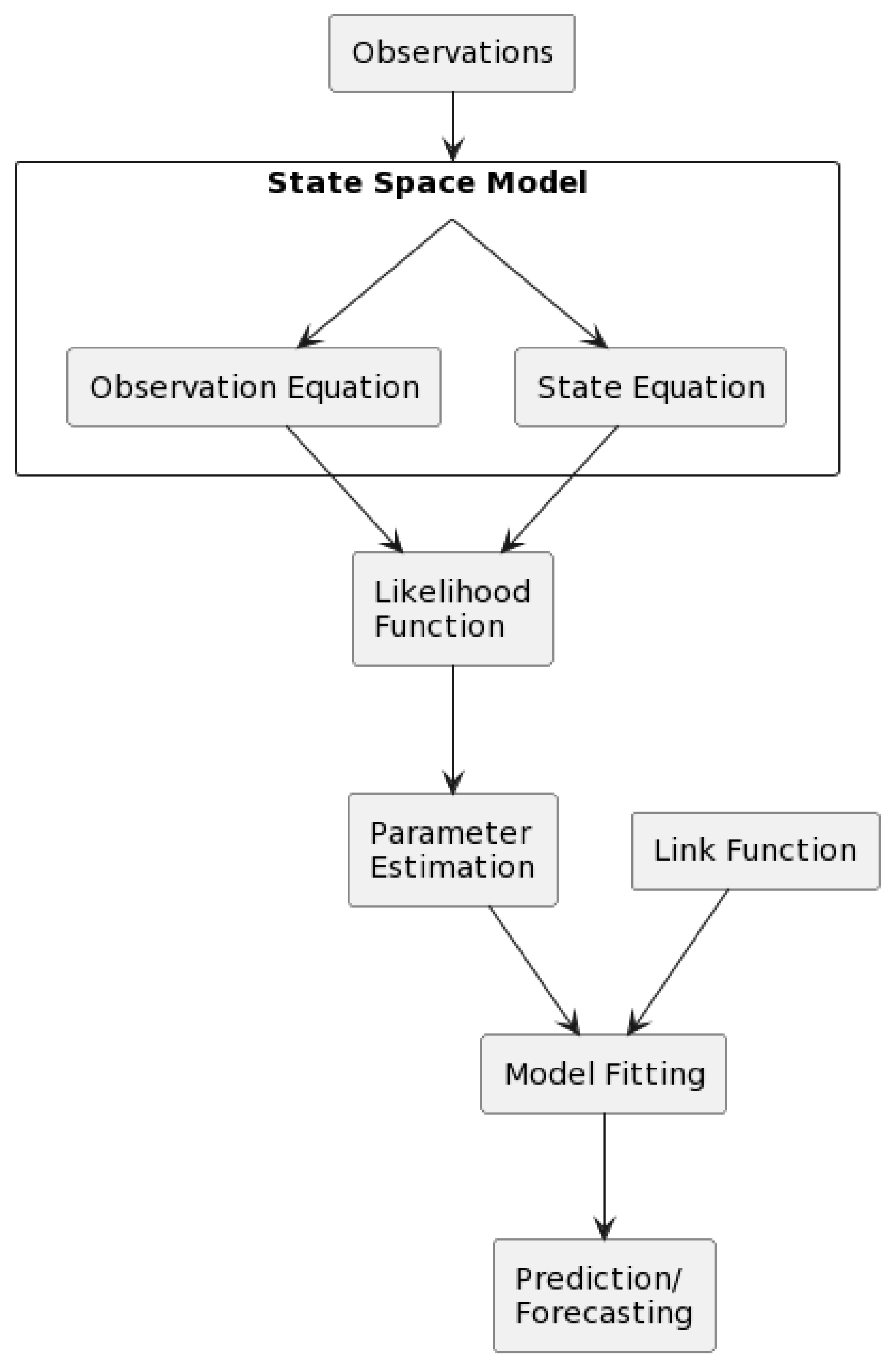
The general fit procedure involves computing ACF and PACF, then applying the Dickey Fuller test to evaluate stationarity. Additionally, we introduce necessary seasonal or order differences to determine the optimal hyperparameters, as outlined by [14].

In the SARIMAX model, the process starts with the time series dataset; therefore, the SARIMAX model could include a seasonal component alongside exogenous variables. Afterwards, several preprocessing steps are implemented (differentiation, scaling, and outliers’ removal) alongside parameter estimation using Akaike Information Criteria (AIC) and Bayesian Information Criteria (BIC) to select the best model. Finally, the trained model is used to forecast new values [68].

2.5.2. DGLM

The Dynamic Generalized Linear Model (DGLM) is an approach based on the prior and posteriori distributions of the data (see Figure 3). If we have a simple model for every timestamp, t is defined as follows:

$$\mathrm{p}\left({\mathrm{Y}}_{\mathrm{t}}|{\mathsf{\eta }}_{\mathrm{t}},\mathsf{\varphi }\right)=\exp \left\{\mathsf{\varphi }\left\{{\mathrm{Y}}_{\mathrm{t}}{\mathsf{\eta }}_{\mathrm{t}}-\mathrm{a}\left({\mathsf{\eta }}_{\mathrm{t}}\right)\right\}\right\}\mathrm{b}\left({\mathrm{Y}}_{\mathrm{t}},\mathsf{\varphi }\right)$$

(2)

where

• ${\mathrm{Y}}_{\mathrm{t}}$ is the random variable at time t;
• $\mathrm{a}\left({\mathsf{\eta }}_{\mathrm{t}}\right)$ is a function of the parameters to adjust the shape of the random variable distribution;
• $\mathrm{b}\left({\mathrm{Y}}_{\mathrm{t}},\mathsf{\varphi }\right)$ represent a normalizing function that ensures the probability distribution integrates (or sums) to 1;
• ${\mathsf{\eta }}_{\mathrm{t}}$ is the natural parameter of the distribution satisfying the following:

  $${\mathrm{E}[\mathrm{Y}}_{\mathrm{t}}\left|{\mathsf{\eta }}_{\mathrm{t}},\mathsf{\varphi }\right]={\mathrm{\mu }}_{\mathrm{t}}=\dot{a\left({\mathsf{\eta }}_{\mathrm{t}}\right)}$$

  (3)
• and $\mathsf{\varphi }$ is a scale parameter with the following:

  $${\mathrm{V}[\mathrm{Y}}_{\mathrm{t}}\left|{\mathsf{\eta }}_{\mathrm{t}},\mathsf{\varphi }\right]=\ddot{a}\left({\mathsf{\eta }}_{\mathrm{t}}\right)/\mathsf{\varphi }$$

  (4)

We also define a conjugate prior for ${\mathsf{\eta }}_{\mathrm{t}}$ named $\mathrm{C}\mathrm{P}[{\mathrm{a}}_{\mathrm{t}},{\mathsf{\beta }}_{\mathrm{t}}]$. Therefore, a dynamic extension of the standard generalized linear model (GLM) can be defined relating ${\mathsf{\eta }}_{\mathrm{t}}$ to the nonlinear transformation ${\mathrm{g}(\mathsf{\eta }}_{\mathrm{t}})$, where g(·) is a link function for simple linear regression given by ${\mathrm{g}(\mathsf{\eta }}_{\mathrm{t}})={\mathsf{\eta }}_{\mathrm{t}}$, with the following structure:

$${\lambda }_t={\mathrm{F}}_{\mathrm{t}}^{\prime }{\theta }_t$$

(5)

where

• ${\lambda }_t$ represents the mean of the response variable;
• ${\mathrm{F}}_{\mathrm{t}}^{\prime }is$ a design matrix or set of features associated with observations;
• ${\theta }_t$ is an underlying state vector having a time evolution similar to that of the DLM. All the mathematical derivations for this model are described by [69].

Figure 3. DGLM architecture.

Figure 3. DGLM architecture.

The DLGM model starts receiving time series data observations. Subsequently, the construction of a state space model delineates the temporal evolution of the system based on its underlying state. Following this, the likelihood function assesses the probability of data observation given specific assumptions (conditional probability). Parameter estimation is then undertaken, while the link function specifies the association between the predictors and the response variable. Afterwards, refinement of the learning process is accomplished through model fitting with the data, facilitating the precise representation of relationships. Ultimately, the dynamic model enables accurate forecasting across diverse contexts [69].

2.5.3. LSTM

Long short-term memory (LSTM) is a variant of a recurrent neural network (RNN) proposed by Hochreiter and Schmidhuber in 1997 [70]. This algorithm solves the long-term dependency problem in RNNs by introducing memory (C) and an appropriate gate structure.

The LSTM cell (Figure 2) has four gates: input ($i$), forget ($f$), control ($c$), and output gates ($o$). The input gate determines the information that can be inserted and transferred to the cell:

$$i_t=\sigma \left(W_i·\left[h_{t-1},x_t\right]+b_i\right)$$

(6)

The forget gate decides which information from the input is important from previous memory as follows:

$$f_t=\sigma \left(W_f·\left[h_{t-1},x_t\right]+b_f\right)$$

(7)

The control gate stabilizes the update in the cell state from $C_{t-1}$ to $C_t$ using Equations (8) and (9):

$$\widetilde{C_t}=\tanh \left(W_C·\left[h_{t-1},x_t\right]+b_c\right)$$

(8)

$$C_t=f_t\times C_{t-1}+\widetilde{C_t}$$

(9)

Additionally, the output gate generates the output, updating the hidden vector $h_{t-1}$ with Equations (10) and (11):

$$o_t={\sigma }_t\times \tanh \left(C_t\right)$$

(10)

$$h_t=o_t\times \tanh \left(C_t\right)$$

(11)

where $\sigma$ is the activation function, W corresponds to the weight matrices calibrated during the training process, tanh is used to scale values in the range of −1 to 1, and b represents the bias in each step. During the training process, the lags ranging from 9 to 15 and the number of cells ranging from 30 to 50 were evaluated to identify the best-performing hyperparameter configuration based on the size and complexity of each dataset. Furthermore, a dense layer is employed as the output layer to facilitate accurate predictions. The latter topology is a common configuration in the LSTM algorithm [71].

To test the prediction’s performance and relative importance, the different scenarios (1, 2, and 3) are defined as follows:

○

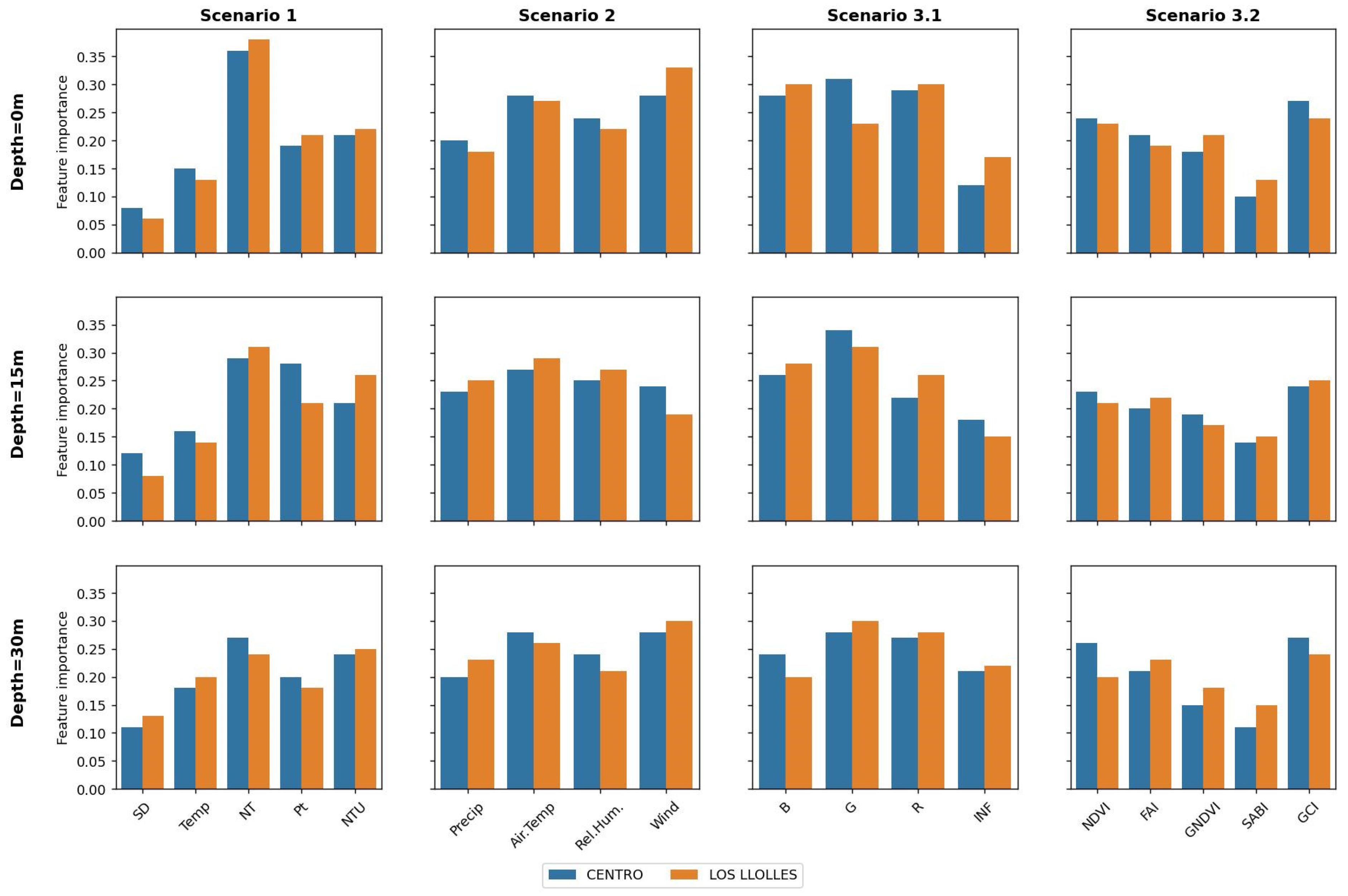
Scenario 1 (measurement data): in the first case, we include the actual variables measured during the monitoring campaigns for the four seasons of the year and in the two seasons of the lake (Chl-a, SD, Temp, NT, Pt, and NTU).

○

Scenario 2 (meteorological variables): in addition to the actual variables, we include meteorological variables as conditioning variables that can influence the autochthonous processes of the lake (precipitation, air temperature, relative humidity, and wind speed).

○

Scenario 3 (satellite data): In this case, we include a sub-case of spectral bands from Landsat satellite processing and another sub-case including vegetation spectral indices.

2.6. Statistics Validation

In Section 2.6, we evaluate the performance of the defined models using several metrics. These metrics include the mean squared error (MSE), as detailed in [72], the root mean squared error (RMSE), as explained in [18], the mean absolute error (MAE), the maximum error, as described in [73], and R², following an approach like the one presented in [14]. These metrics provide information on the accuracy, precision, and potential limitations of the chlorophyll-a estimation.

The dataset was divided into training and test datasets, with details provided in

Table 3. Training and test datasets used in the statistical and machine learning models.

Station/Depth	0 M (Train/Test)	15 M (Train/Test)	30 M (Train/Test)
CENTRO	38/16	38/16	38/16
LOS LOLLES	28/12	28/12	28/12

. A sequential splitting method was employed, following the 70/30% rule, to calculate the various error metrics. In this approach, the time series data were divided into two segments: the first part was used for model training, while the latter was used for model validation. This strategy was applied to different monitoring stations (see Figure 1) and has been shown to provide good performance for evaluating the performance of deep learning models in time series analysis [74,75].

3. Results

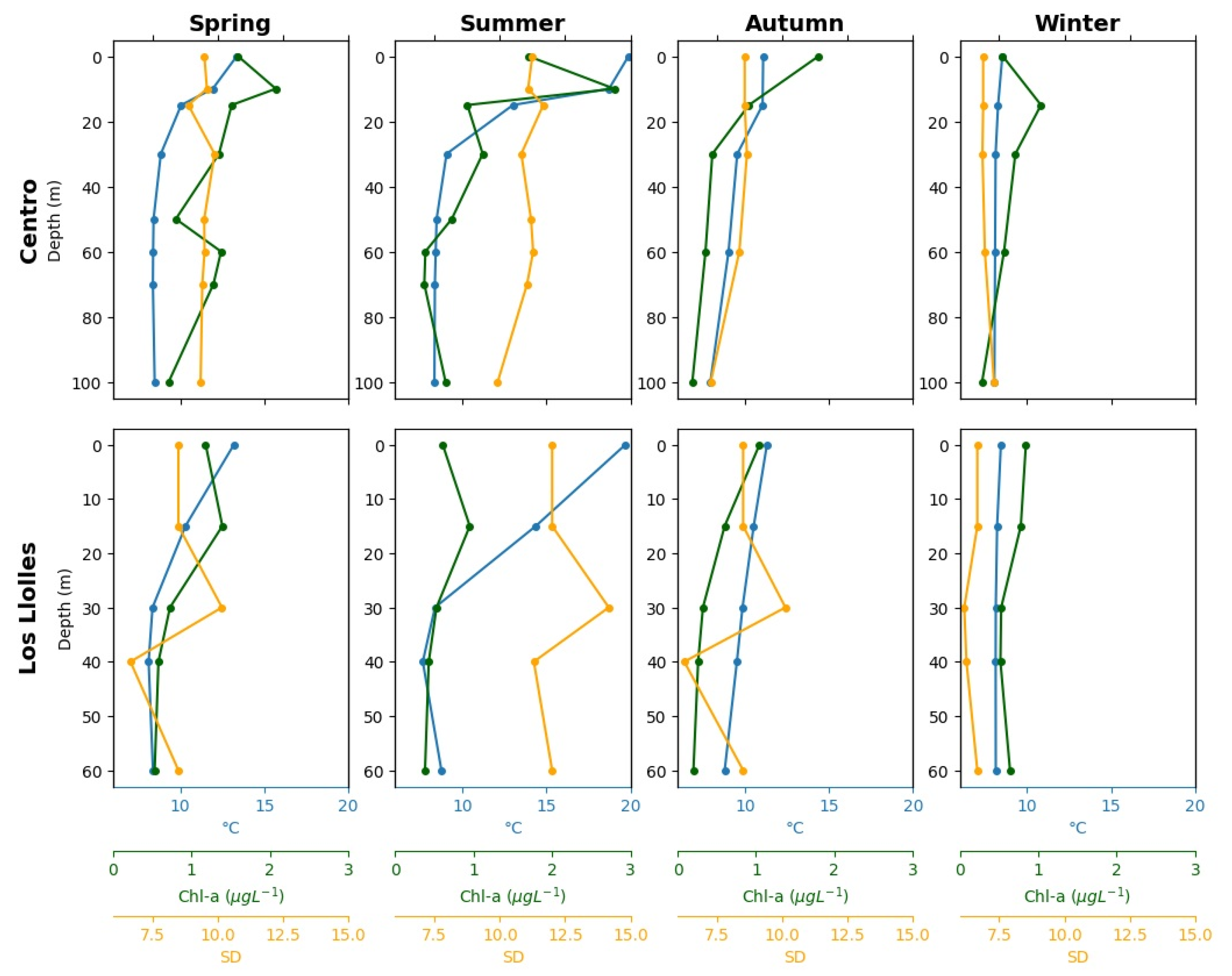
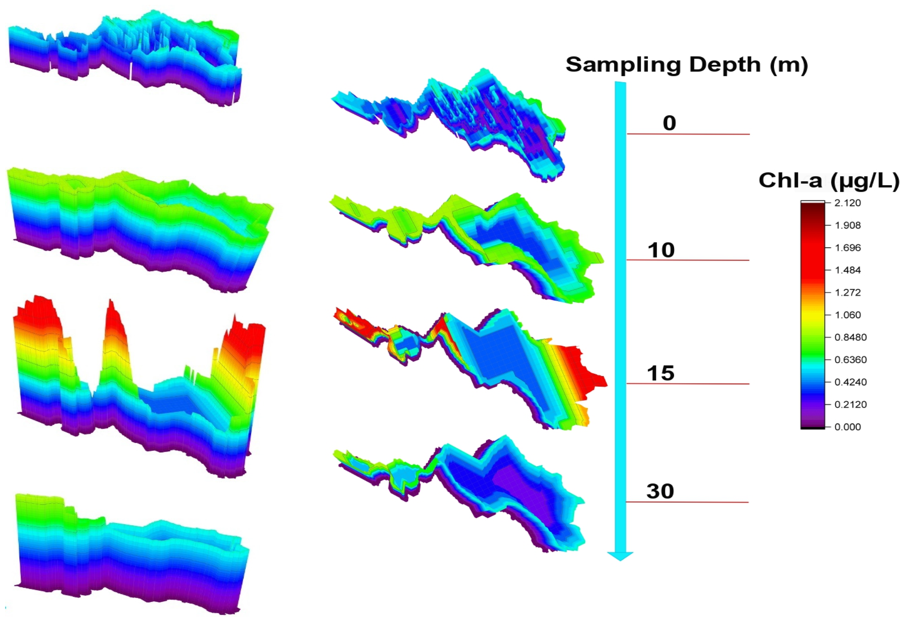
3.1. Behavior of Chl-a, SD, and T Values at Depth

Figure 4 shows the behavior of limnological parameters during the study period (2001–2020) at different depths for two stations of Lake Maihue during the four seasons of the year. The Chl-a values range from a maximum of 3.10 (µg/L) in the summer season and a maximum of 2.59 in the spring since these seasons are the most productive due to their seasonal characteristics, where there is a higher water temperature and hydrodynamic stability of the lake, to minimum values of 0.2 (µg/L) in the winter. Transparency varies between maximums of 19.5 m according to the Secchi disk in the summer due to the great penetration of solar radiation at depth and minimum values of 2.30 m in winter and autumn due to the mixing present in the lake by rainfall, strong winds, and the turbidity generated by these conditions in the water. The minimum temperature is 7.96 degrees in the winter, and in the summer, it reaches 21.98 degrees, which is quite high for these latitudes, a possible effect of the increases attributed to the surface temperature in lakes due to the current climate crisis. Figure 5 shows the spatial behavior of Chl-a at different depths. For more details of the limnological parameters, see Tables S1–S4.

3.2. Important Features

Figure 6 shows, using the Garson weighting method [76], the relative importance or contribution of the independent variables (predictor variables) in explaining the variance of the dependent variable (result variable) for each of the cases used.

The results showed that total nitrogen (NT), total phosphorus (Pt), and turbidity (NTU) present the highest values of relative importance (ranging between 0.20 and 0.29) in the prediction of chlorophyll-a in the two stations of Case 1. Subsequently, air temperature (Air. Temp) and wind (Wind) showed relative importance, ranging between 0.28 and 0.31, with wind being more significant than air temperature. On the contrary, transparency (SD), relative humidity (Real.Hum), and precipitation (Precip) show relatively minor importance, with all values lower than 0.20.

In the last two scenarios, where the satellite bands were used independently (Scenario 3.1) and the vegetation indices (Scenario 3.2), they showed a high importance in the prediction of Chl-a, with values higher than 0.18 in all cases. The independent bands green (G) and red (red) proved to be the ones that best explain the behavior of the variable for Lake Maihue, with values above 0.28 in all cases.

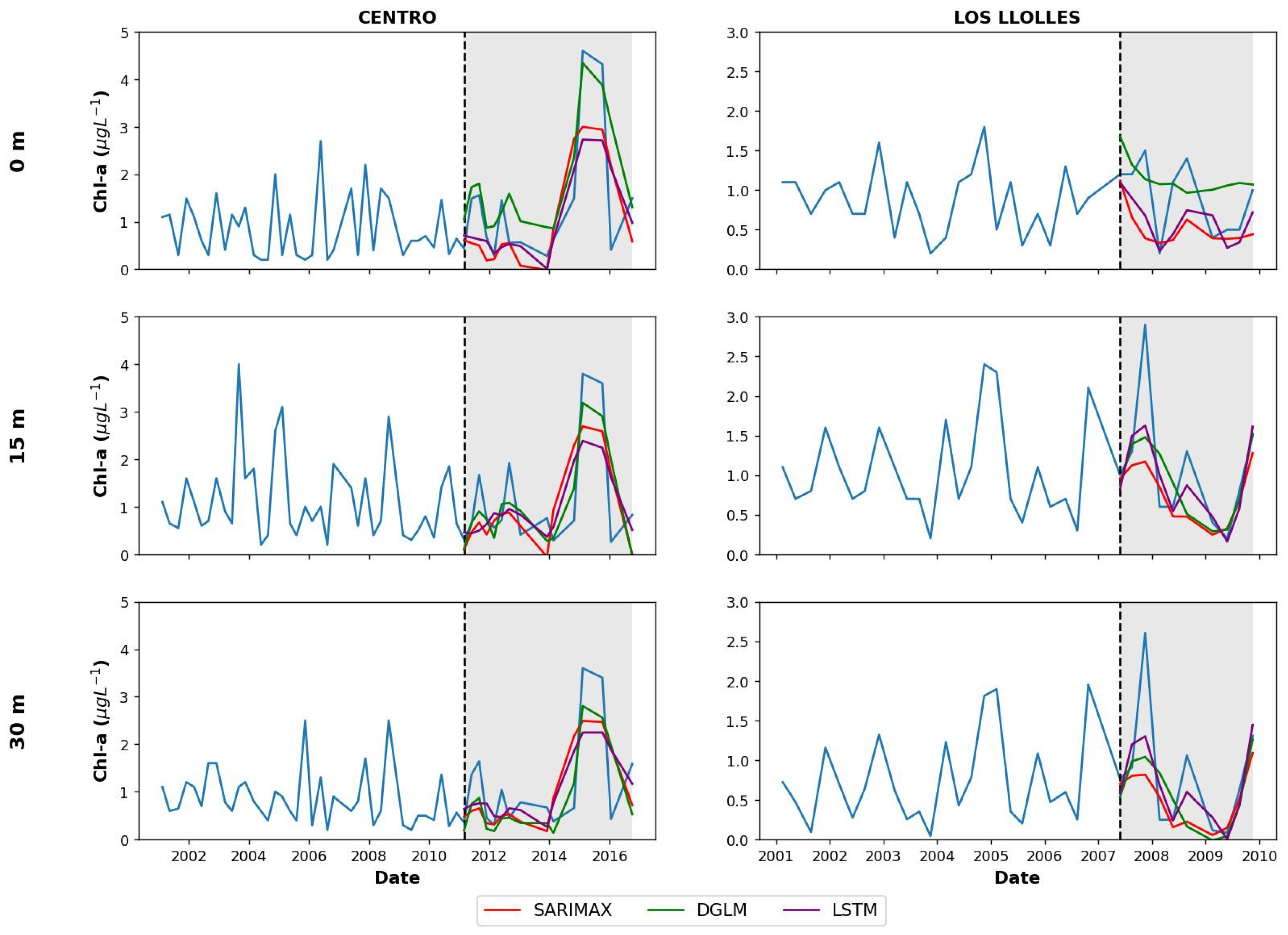
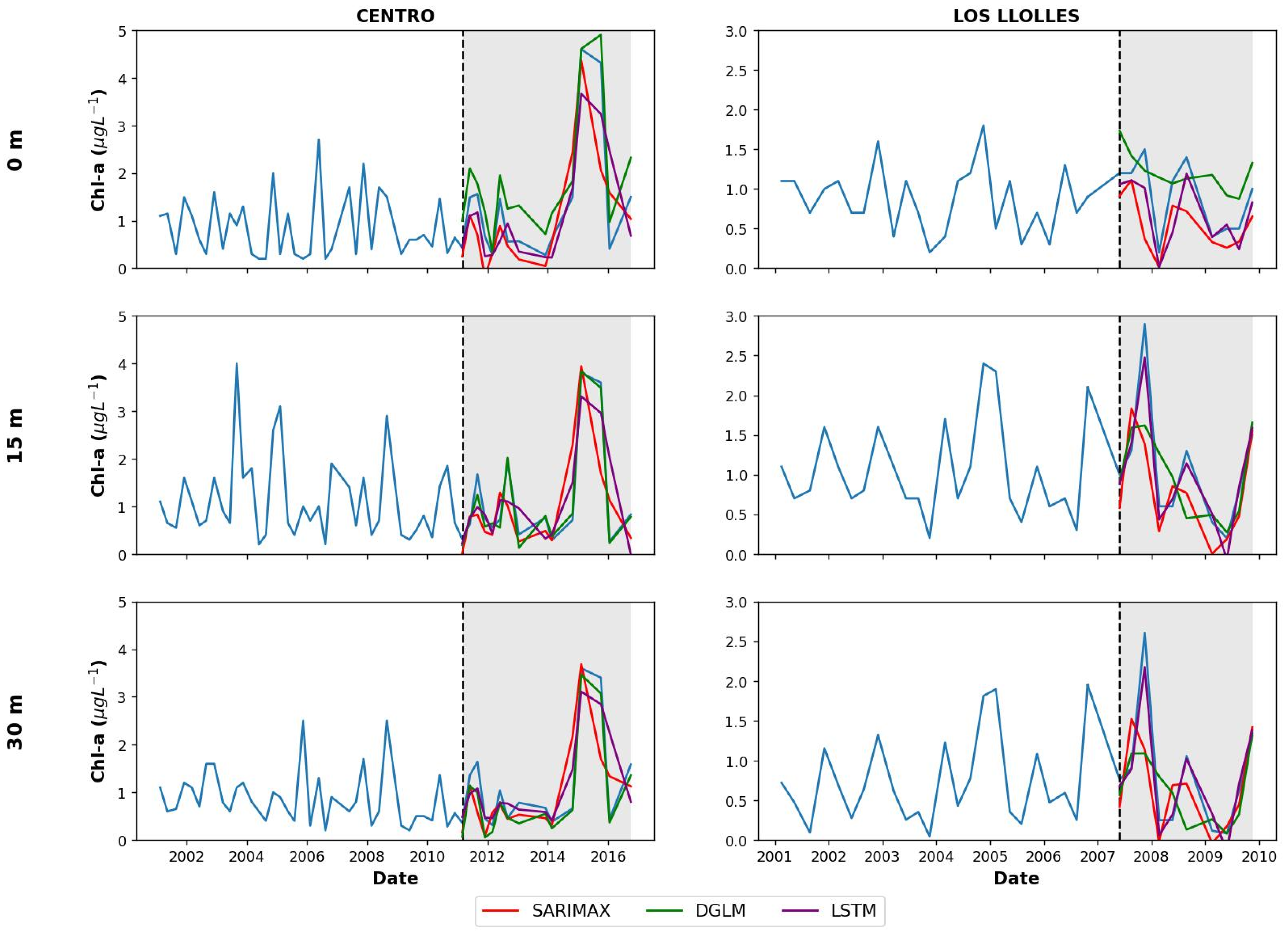
3.3. Chl-a Estimation Scenarios

Scenario 1. In situ variables (Chl-a, SD, Temp, NT, Pt, NTU)

The temporal variations in the concentration of chlorophyll measured in situ and derived from statistical and machine learning techniques at different depths (0 m, 15 m, and 30 m) and for two stations (CENTRO and LOS LLOLLES) are presented in Figure 7. The performances of these methods using the metrics described in Section 2.6 are presented in

Table 4. Validation metrics for all the stations and models considered in Scenario 1.

Model/Station	Station	Depth	MSE (μg/L) ²	RMSE (μg/L)	MaxError (μg/L)	MAE (μg/L)	R2
SARIMAX	CENTRO	0 m	0.90	0.95	2.59	0.94	0.35
		15 m	0.73	0.85	2.38	0.98	0.34
		30 m	0.66	0.81	2.37	0.92	0.32
	LOS LLOLLES	0 m	0.30	0.55	1.11	0.41	0.30
		15 m	0.39	0.62	1.73	0.38	0.43
		30 m	0.41	0.64	1.79	0.36	0.35
DGLM	CENTRO	0 m	0.72	0.85	2.68	0.59	0.57
		15 m	0.47	0.69	1.74	0.54	0.61
		30 m	0.46	0.68	1.55	0.55	0.58
	LOS LLOLLES	0 m	0.24	0.49	0.94	0.42	0.50
		15 m	0.33	0.57	1.42	0.37	0.47
		30 m	0.43	0.66	1.67	0.45	0.38
LSTM	CENTRO	0 m	0.82	0.91	1.87	0.66	0.52
		15 m	0.69	0.83	1.41	0.66	0.43
		30 m	0.60	0.77	1.46	0.63	0.58
	LOS LLOLLES	0 m	0.19	0.43	0.82	0.35	0.37
		15 m	0.21	0.46	1.28	0.29	0.61
		30 m	0.23	0.48	1.30	0.32	0.65

. SARIMAX and LSTM exhibit a broader dispersion range, with MSE values spanning from 0.30 to 0.90 and 0.19 to 0.82, respectively, across all depths and stations. Conversely, DLGM demonstrates a lower spread, with MSE values ranging from 0.24 to 0.72, with very good performance at 15 m depth. It is noteworthy that the most significant performance deficit for the CENTRO (LOS LLOLLES) station is observed at 0 (30) m depth, characterized by elevated MSE, RMSE, max error, and MAE metrics.

Additionally, R² values reveal diverse trends, spanning from 0.30 to 0.65, with DLGM and LSTM models exhibiting superior values compared to SARIMAX performance (Table 4). It is important to note that R² is an estimator significantly influenced by outliers, as evidenced in this instance in the test data considered for the analysis. Consequently, it cannot be solely relied upon as an exclusive performance indicator.

Overall, LSTM and DGLM perform better than SARIMAX at the CENTRO station. Conversely, SARIMAX appears to be a viable alternative for the LOS LLOLLES station. However, the choice between them depends on specific depth and station requirements, with LSTM (DGLM) performing well at CENTRO (LOS LLOLLES), with better results at 15 m depth.

Scenario 2. Meteorological variables (precipitation, air temperature, relative humidity, and wind speed)

Time variations in chlorophyll concentration measured in situ and obtained from statistical and machine learning techniques at different depths (0 m, 15 m, and 30 m) and for two stations (CENTRO and LOS LLOLLES) are presented in Figure 8. The performances of these methods using the statistical metrics described in Section 2.6 are presented in

Table 5. Validation metrics for all the stations and models considered in Scenario 2.

Model/Station	Station	Depth	MSE (μg/L) ²	RMSE (μg/L)	MaxError (μg/L)	MAE (μg/L)	R2
SARIMAX	CENTRO	0 m	0.65	0.81	3.96	0.93	0.32
		15 m	0.62	0.79	3.54	0.96	0.31
		30 m	0.52	0.72	3.57	0.88	0.29
	LOS LLOLLES	0 m	0.22	0.47	1.13	0.35	0.54
		15 m	0.34	0.59	1.51	0.43	0.65
		30 m	0.35	0.59	1.57	0.42	0.52
DGLM	CENTRO	0 m	0.28	0.53	0.82	0.47	0.84
		15 m	0.03	0.16	0.43	0.13	0.98
		30 m	0.08	0.28	0.64	0.23	0.93
	LOS LLOLLES	0 m	0.24	0.49	0.94	0.42	0.50
		15 m	0.32	0.56	1.28	0.41	0.43
		30 m	0.42	0.65	1.62	0.43	0.46
LSTM	CENTRO	0 m	0.57	0.76	2.06	0.55	0.67
		15 m	0.47	0.68	1.77	0.53	0.62
		30 m	0.39	0.62	1.82	0.43	0.65
	LOS LLOLLES	0 m	0.09	0.29	0.65	0.22	0.55
		15 m	0.04	0.19	0.42	0.16	0.93
		30 m	0.03	0.19	0.43	0.14	0.94

.

The DLGM model performed very well at the CENTRO station, with R² values between 0.84 and 0.93 and MSE values between 0.03 and 0.28, presenting a higher degree of correspondence at 15 m depth. Furthermore, LSTM excels as the most performant model at the LOS LLOLLES station, with notable lower MSE values compared to the other two models, ranging from 0.03 to 0.09, and higher correlations (up to 0.94 at 30 m depth) (Table 5). Overall, LSTM exhibited better performance error metrics compared to SARIMAX (Table 5).

Scenario 3. Satellite data:

3.1 Spectral Bands (B, G, R, and INR).

Seasonal fluctuations in chlorophyll concentration, evaluated in situ and extrapolated using statistical and machine learning techniques at various depths (0 m, 15 m, and 30 m) and for two stations (CENTRO and LOS LLOLLES), are presented in Figure 9. The performance of these methods, evaluated based on the statistical metrics described in Section 2.6, is illustrated in

Table 6. Validation metrics for all the stations and models considered in Scenario 3.1.

Model/Station	Station	Depth	MSE (μg/L) ²	RMSE (μg/L)	MaxError (μg/L)	MAE (μg/L)	R2
SARIMAX	CENTRO	0 m	0.60	0.77	3.20	0.93	0.33
		15 m	0.47	0.69	2.81	0.96	0.30
		30 m	0.39	0.63	2.88	0.94	0.29
	LOS LLOLLES	0 m	0.19	0.44	0.86	0.36	0.38
		15 m	0.22	0.47	1.34	0.29	0.58
		30 m	0.43	0.49	1.33	0.33	0.54
DGLM	CENTRO	0 m	0.87	0.93	1.96	0.75	0.48
		15 m	0.61	0.78	1.76	0.55	0.49
		30 m	0.52	0.73	01.75	0.53	0.48
	LOS LLOLLES	0 m	0.30	0.55	0.95	0.46	0.32
		15 m	0.35	0.59	1.40	0.39	0.46
		30 m	0.43	0.66	1.61	0.42	0.45
LSTM	CENTRO	0 m	0.81	0.90	1.94	0.73	0.52
		15 m	0.73	0.85	1.84	0.68	0.39
		30 m	0.63	0.80	1.75	0.63	0.38
	LOS LLOLLES	0 m	0.15	0.38	1.04	0.24	0.42
		15 m	0.29	0.54	1.41	0.41	0.44
		30 m	0.28	0.53	1.33	0.39	0.56

. SARIMAX showed a good performance at the CENTRO station across all depths. DGLM presented slightly higher MSE values compared to SARIMAX, with lower RMSE values at 15 m depth. LSTM also showed good performance metrics, with MSE values ranging from 0.15 to 0.81; however, it did not perform well in the LOS LLOLLES station at 15 m.

3.2 Scenario 3.2. Vegetation Indices

Temporal fluctuations in chlorophyll concentration, evaluated in situ and extrapolated using statistical and machine learning techniques at various depths (0 m, 15 m, and 30 m) and for two stations (CENTRO and LOS LLOLLES), are presented in Figure 10. The effectiveness of these methods, evaluated based on the statistical metrics described in Section 2.6, is illustrated in

Table 7. Validation metrics for all the stations and models considered in Scenario 3.2.

Model/Station	Station	Depth	MSE (μg/L) ²	RMSE (μg/L)	MaxError (μg/L)	MAE (μg/L)	R2
SARIMAX	CENTRO	0 m	0.69	0.82	2.67	0.91	0.30
		15 m	0.67	0.82	2.43	0.98	0.32
		30 m	0.59	0.71	2.42	0.98	0.36
	LOS LLOLLES	0 m	0.19	0.43	0.79	0.35	0.35
		15 m	0.29	0.54	1.21	0.41	0.47
		30 m	0.32	0.57	1.29	0.42	0.39
DGLM	CENTRO	0 m	0.42	0.65	1.19	0.57	0.75
		15 m	0.22	0.47	0.85	0.41	0.82
		30 m	0.17	0.42	0.77	0.34	0.83
	LOS LLOLLES	0 m	0.26	0.51	1.07	0.42	0.38
		15 m	0.35	0.59	1.40	0.39	0.46
		30 m	0.48	0.69	1.88	0.44	0.48
LSTM	CENTRO	0 m	0.74	0.86	2.01	0.59	0.57
		15 m	0.68	0.82	1.88	0.66	0.44
		30 m	0.59	0.76	1.85	0.59	0.46
	LOS LLOLLES	0 m	0.15	0.38	1.04	0.24	0.42
		15 m	0.22	0.47	1.08	0.36	0.59
		30 m	0.24	0.49	1.13	0.36	0.57

. In general, a better performance can be observed at the LOS LLOLLES station when compared to the performance at the CENTRO station. The best performance is observed at 15 m with SARIMAX, and the DGLM model showed the better performance metrics.

4. Discussion

The remote lakes of the Andes have long been an enigma in terms of historical information on the limnological characteristics of their waters. In this context, our study of Lake Maihue has emerged as a beacon of knowledge, allowing us to obtain valuable data on the current state of water quality and the evolution of its algal community. Our approach involved an assessment through three different scenarios: Scenario 1 (field measurement data), Scenario 2 (meteorological data), and Scenario 3 (satellite data). Through these scenarios, we have employed three deep learning and traditional statistical models to estimate the behavior of the variable Chl-a, taking advantage of the richness of data offered by these parameters. The models used for the estimation of Chl-a, SARIMAX, DGLM, and LSTM, have proven their effectiveness in various applications and were successfully employed in our study.

From the results obtained, we can observe that Scenario 2 exhibits better performance metrics, with lower MSE/RMSE values and higher R² scores than the other ones, with both LSTM and DGLM as the best models across various stations and depths. Scenario 1, on the contrary, although also presenting low MSE and RMSE values, generally exhibits slightly lower R² scores than those in Scenario 2. Additionally, Scenarios 3.1 and 3.2 showed slightly higher MSE and RMSE values compared to Scenarios 1 and 2. Overall, DGLM and LSTM consistently demonstrated better performance regarding the depths and stations analyzed. In contrast, the SARIMAX performance was the worst, probably due to the difficulties in dealing with non-linearities present in the test data. DGLM and LSTM appear particularly effective in cases involving non-stationary time series, a common characteristic among the series in this study. Notably, the performance tends to improve with increasing depth, with notably better metrics at 15 m. The results obtained have shed light on the superior performance of Scenario 2, supported by more favorable metrics such as lower MSE/RMSE values and higher R² scores (see Table 2, Table 3, Table 4 and Table 5). In this scenario, LSTM and DGLM stand out as the outstanding models not only at one but also at multiple stations and depths.

Overall, the DLGM model demonstrates superior performance at the CENTRO station, whereas LSTM excels at the LOS LLOLLES station. This outcome aligns with expectations, given the presence of significant outliers in the test data that were not observed in the training data. It is noteworthy that SARIMAX, unlike the DLGM and LSTM models, is limited in its ability to handle such non-linearities.

In addition, it is relevant to mention that the performance tends to improve as depth increases, with significantly more favorable metrics at 15 m depth, where a higher concentration of Chl-a is observed, indicating the presence of algae.

The results of our study reveal that Lake Maihue has experienced a slight increase in Chl-a concentration during the study period, which spans from 2001 to 2020. Our work is part of a series of investigations carried out in lakes in the Chilean mountain range, in which the evolution of algal activity has been closely followed. For example, in a previous study [13] in Lake Laja, the phenomenon of algal blooms was documented. Likewise, another recent study [15] in Lake Villarrica identified a close relationship between these blooms and changing meteorological conditions, directly related to algal blooms. In Lake Llanquihue, artificial intelligence models were tested to estimate the concentration of chlorophyll-a before other parameters because several regional capitals are in this lake, which contribute to accelerating the impacts on the water quality of this lake system with the multiple uses of this aquatic ecosystem.

Remote sensing has proven to be a valuable tool in the monitoring of lake systems in the mountain range of this South American country and a relevant element in the monitoring of the current state of the water resource as well as the evolution of algae. In this research, the best predictions were obtained with meteorological data rather than satellite data, but this may be a consequence of the insufficient spatial distribution of in situ data. Therefore, in future research, it is intended to have more monitoring stations and carry out modeling with the greatest amount of combined data, including in situ, meteorological, and satellite data in the same model. Our future projection in this direction is to increase the data on water quality parameters and, thus, improve the prediction of deep learning models using a combination of remote sensing data, meteorological data, and field campaigns. Caring for lake water quality is essential to protecting human health, biodiversity, the local economy, and the environment in general. It is vital to take measures to prevent pollution and promote sustainable management of these valuable water resources.

5. Conclusions

The employment of in situ, meteorological, and remote sensing data has been highlighted as a valuable resource for estimating environmental indicators, such as chlorophyll-a at different depths. This parameter has been widely used in various aquatic ecosystems to assess both algal biomass and water quality, but at depth, it is a novel contributor. In this study, a set of in situ data collected between 2001 and 2020 at two monitoring stations in Lake Maihue was used to analyze the behavior of limnological variables in different areas of the lake.

The results of this study revealed that the three estimation models used demonstrated an effective ability to predict chlorophyll-a concentration, with the LSTM and DGLM models standing out as the most accurate ones compared to the SARIMAX model.

Of the four scenarios evaluated in this study, Scenario 2 exhibits better performance metrics, yielding the most accurate results for the analyzed stations and depths in the lake. These models will be fundamental tools for future research, especially during the autumn and winter seasons, when episodes of rain and strong winds, such as the Puelches winds, are common and conventional monitoring is more complex. Consequently, there is a need to use estimation models, such as those presented in this study, that combine real data with meteorological and remote sensing data using deep learning tools.

References

1. Moser, K.A.; Baron, J.S.; Brahney, J.; Oleksy, I.A.; Saros, J.E.; Hundey, E.J.; Sadro, S.A.; Kopáček, J.; Sommaruga, R.; Kainz, M.J.; et al. Mountain Lakes: Eyes on Global Environmental Change. Glob. Planet. Change 2019, 178, 77–95. [Google Scholar] [CrossRef]
2. Tong, H.-L.; Shi, P.-J. Using Ecosystem Service Supply and Ecosystem Sensitivity to Identify Landscape Ecology Security Patterns in the Lanzhou-Xining Urban Agglomeration, China. J. Mt. Sci. 2020, 17, 2758–2773. [Google Scholar] [CrossRef]
3. Grebby, S.; Sowter, A.; Gee, D.; Athab, A.; De la Barreda-Bautista, B.; Girindran, R.; Marsh, S. Remote Monitoring of Ground Motion Hazards in High Mountain Terrain Using Insar: A Case Study of the Lake Sarez Area, Tajikistan. Appl. Sci. 2021, 11, 8738. [Google Scholar] [CrossRef]
4. Regmi, G.R.; Huettmann, F. Hindu Kush-Himalaya Watersheds Downhill: Landscape Ecology and Conservation Perspectives; Springer International Publishing: Cham, Switzerland, 2020; ISBN 9783030362751. [Google Scholar]
5. Wolf, I.D.; Croft, D.B.; Green, R.J. Nature Conservation and Nature-Based Tourism: A Paradox? Environments 2019, 6, 104. [Google Scholar] [CrossRef]
6. Danilov-Danilyan, V.I.; Klyuev, N.N.; Kotlyakov, V.M. Russia in the Global Natural and Ecological Space. Reg. Res. Russ. 2023, 13, 34–57. [Google Scholar] [CrossRef]
7. Paltsev, A.; Creed, I.F. Are Northern Lakes in Relatively Intact Temperate Forests Showing Signs of Increasing Phytoplankton Biomass? Ecosystems 2021, 25, 727–755. [Google Scholar] [CrossRef]
8. Pritsch, H.; Schirpke, U.; Jersabek, C.D.; Kurmayer, R. Plankton Community Composition in Mountain Lakes and Consequences for Ecosystem Services. Ecol. Indic. 2023, 154, 110532. [Google Scholar] [CrossRef]
9. De los Ríos-Escalante, P.R.; Woelfl, S. A Review of Zooplankton Research in Chile. Limnologica 2023, 100, 126079. [Google Scholar] [CrossRef]
10. Tovar-Sánchez, A.; Román, A.; Roque-Atienza, D.; Navarro, G. Applications of Unmanned Aerial Vehicles in Antarctic Environmental Research. Sci. Rep. 2021, 11, 21717. [Google Scholar] [CrossRef] [PubMed]
11. Kallenbach, E.M.F.; Friberg, N.; Lusher, A.; Jacobsen, D.; Hurley, R.R. Anthropogenically Impacted Lake Catchments in Denmark Reveal Low Microplastic Pollution. Environ. Sci. Pollut. Res. 2022, 29, 47726–47739. [Google Scholar] [CrossRef] [PubMed]
12. Cantonati, M.; Poikane, S.; Pringle, C.M.; Stevens, L.E.; Turak, E.; Heino, J.; Richardson, J.S.; Bolpagni, R.; Borrini, A.; Cid, N.; et al. Characteristics, Main Impacts, and Stewardship of Natural and Artificial Freshwater Environments: Consequences for Biodiversity Conservation. Water 2020, 12, 260. [Google Scholar] [CrossRef]
13. Rodríguez-López, L.; Duran-Llacer, I.; González-Rodríguez, L.; Abarca-del-Rio, R.; Cárdenas, R.; Parra, O.; Martínez-Retureta, R.; Urrutia, R. Spectral Analysis Using LANDSAT Images to Monitor the Chlorophyll-a Concentration in Lake Laja in Chile. Ecol. Inform. 2020, 60, 101183. [Google Scholar] [CrossRef]
14. Rodríguez-López, L.; Usta, D.B.; Duran-Llacer, I.; Alvarez, L.B.; Yépez, S.; Bourrel, L.; Frappart, F.; Urrutia, R. Estimation of Water Quality Parameters through a Combination of Deep Learning and Remote Sensing Techniques in a Lake in Southern Chile. Remote Sens. 2023, 15, 4157. [Google Scholar] [CrossRef]
15. Rodríguez-López, L.; Duran-Llacer, I.; Bravo Alvarez, L.; Lami, A.; Urrutia, R. Recovery of Water Quality and Detection of Algal Blooms in Lake Villarrica through Landsat Satellite Images and Monitoring Data. Remote Sens. 2023, 15, 1929. [Google Scholar] [CrossRef]
16. Rodríguez-López, L.; Bustos Usta, D.; Bravo Alvarez, L.; Duran-Llacer, I.; Lami, A.; Martínez-Retureta, R.; Urrutia, R. Machine Learning Algorithms for the Estimation of Water Quality Parameters in Lake Llanquihue in Southern Chile. Water 2023, 15, 1994. [Google Scholar] [CrossRef]
17. Park, J.; Kim, K.T.; Lee, W.H. Recent Advances in Information and Communications Technology (ICT) and Sensor Technology for Monitoring Water Quality. Water 2020, 12, 510. [Google Scholar] [CrossRef]
18. Rodríguez-López, L.; González-Rodríguez, L.; Duran-Llacer, I.; Cardenas, R.; Urrutia, R. Spatio-Temporal Analysis of Chlorophyll in Six Araucanian Lakes of Central-South Chile from Landsat Imagery. Ecol. Inform. 2021, 65, 101431. [Google Scholar] [CrossRef]
19. Skakun, S.; Kalecinski, N.I.; Brown, M.G.L.; Johnson, D.M.; Vermote, E.F.; Roger, J.C.; Franch, B. Assessing Within-Field Corn and Soybean Yield Variability from Worldview-3, Planet, Sentinel-2, and Landsat 8 Satellite Imagery. Remote Sens. 2021, 13, 872. [Google Scholar] [CrossRef]
20. Vrdoljak, L.; Kilić Pamuković, J. Assessment of Atmospheric Correction Processors and Spectral Bands for Satellite-Derived Bathymetry Using Sentinel-2 Data in the Middle Adriatic. Hydrology 2022, 9, 215. [Google Scholar] [CrossRef]
21. Legleiter, C.J.; King, T.V.; Carpenter, K.D.; Hall, N.C.; Mumford, A.C.; Slonecker, T.; Graham, J.L.; Stengel, V.G.; Simon, N.; Rosen, B.H. Spectral Mixture Analysis for Surveillance of Harmful Algal Blooms (SMASH): A Field-, Laboratory-, and Satellite-Based Approach to Identifying Cyanobacteria Genera from Remotely Sensed Data. Remote Sens. Environ. 2022, 279, 113089. [Google Scholar] [CrossRef]
22. de Lima, T.M.A.; Giardino, C.; Bresciani, M.; Barbosa, C.C.F.; Fabbretto, A.; Pellegrino, A.; Begliomini, F.N. Assessment of Estimated Phycocyanin and Chlorophyll-a Concentration from PRISMA and OLCI in Brazilian Inland Waters: A Comparison between Semi-Analytical and Machine Learning Algorithms. Remote Sens. 2023, 15, 1299. [Google Scholar] [CrossRef]
23. Zhang, H.; Xue, B.; Wang, G.; Zhang, X.; Zhang, Q. Deep Learning-Based Water Quality Retrieval in an Impounded Lake Using Landsat 8 Imagery: An Application in Dongping Lake. Remote Sens. 2022, 14, 4505. [Google Scholar] [CrossRef]
24. Gómez, D.; Salvador, P.; Sanz, J.; Casanova, J.L. A New Approach to Monitor Water Quality in the Menor Sea (Spain) Using Satellite Data and Machine Learning Methods. Environ. Pollut. 2021, 286, 117489. [Google Scholar] [CrossRef] [PubMed]
25. Chusnah, W.N.; Chu, H.J.; Tatas; Jaelani, L.M. Machine-Learning-Estimation of High-Spatiotemporal-Resolution Chlorophyll-a Concentration Using Multi-Satellite Imagery. Sustain. Environ. Res. 2023, 33, 11. [Google Scholar] [CrossRef]
26. Medina-López, E.; Navarro, G.; Santos-Echeandía, J.; Bernárdez, P.; Caballero, I. Machine Learning for Detection of Macroalgal Blooms in the Mar Menor Coastal Lagoon Using Sentinel-2. Remote Sens. 2023, 15, 1208. [Google Scholar] [CrossRef]
27. Berger, K.; Rivera Caicedo, J.P.; Martino, L.; Wocher, M.; Hank, T.; Verrelst, J. A Survey of Active Learning for Quantifying Vegetation Traits from Terrestrial Earth Observation Data. Remote Sens. 2021, 13, 287. [Google Scholar] [CrossRef] [PubMed]
28. Nasir, N.; Kansal, A.; Alshaltone, O.; Barneih, F.; Shanableh, A.; Al-Shabi, M.; Al Shammaa, A. Deep Learning Detection of Types of Water-Bodies Using Optical Variables and Ensembling. Intell. Syst. Appl. 2023, 18, 200222. [Google Scholar] [CrossRef]
29. Sadaiappan, B.; Balakrishnan, P.; Vishal, C.R.; Vijayan, N.T.; Subramanian, M.; Gauns, M.U. Applications of Machine Learning in Chemical and Biological Oceanography. ACS Omega 2023, 8, 15831–15853. [Google Scholar] [CrossRef] [PubMed]
30. Peterson, K.T.; Sagan, V.; Sidike, P.; Hasenmueller, E.A.; Sloan, J.J.; Knouft, J.H. Machine Learning-Based Ensemble Prediction of Water-Quality Variables Using Feature-Level and Decision-Level Fusion with Proximal Remote Sensing. Photogramm. Eng. Remote Sens. 2019, 85, 269–280. [Google Scholar] [CrossRef]
31. Herng, Y.; Wai, K.; Shen, B.; Chun, A.; Loy, M.; Shahbaz, M.; Kaur, H.; Singh, G.; Yusuf, R.; Fadzil, A.; et al. Science of the Total Environment An Overview of Biomass Thermochemical Conversion Technologies in Malaysia. Sci. Total Environ. 2019, 680, 105–123. [Google Scholar] [CrossRef]
32. Pahlevan, N.; Smith, B.; Schalles, J.; Binding, C.; Cao, Z.; Ma, R.; Alikas, K.; Kangro, K.; Gurlin, D.; Hà, N.; et al. Seamless Retrievals of Chlorophyll-a from Sentinel-2 (MSI) and Sentinel-3 (OLCI) in Inland and Coastal Waters: A Machine-Learning Approach. Remote Sens. Environ. 2020, 240, 111604. [Google Scholar] [CrossRef]
33. Su, H.; Lu, X.; Chen, Z.; Zhang, H.; Lu, W.; Wu, W. Estimating Coastal Chlorophyll-a Concentration from Time-Series Olci Data Based on Machine Learning. Remote Sens. 2021, 13, 576. [Google Scholar] [CrossRef]
34. Li, H.; Qin, C.; He, W.; Sun, F.; Du, P. Improved Predictive Performance of Cyanobacterial Blooms Using a Hybrid Statistical and Deep-Learning Method. Environ. Res. Lett. 2021, 16, 124045. [Google Scholar] [CrossRef]
35. Nguyen, H.Q.; Ha, N.T.; Nguyen-Ngoc, L.; Pham, T.L. Comparing the Performance of Machine Learning Algorithms for Remote and in Situ Estimations of Chlorophyll-a Content: A Case Study in the Tri an Reservoir, Vietnam. Water Environ. Res. 2021, 93, 2941–2957. [Google Scholar] [CrossRef]
36. Kolluru, S.; Tiwari, S.P. Modeling Ocean Surface Chlorophyll-a Concentration from Ocean Color Remote Sensing Reflectance in Global Waters Using Machine Learning. Sci. Total Environ. 2022, 844, 157191. [Google Scholar] [CrossRef]
37. Bartold, M.; Kluczek, M. A Machine Learning Approach for Mapping Chlorophyll Fluorescence at Inland Wetlands. Remote Sens. 2023, 15, 2392. [Google Scholar] [CrossRef]
38. Caballero, I.; Fernández, R.; Escalante, O.M.; Mamán, L.; Navarro, G. New Capabilities of Sentinel-2A/B Satellites Combined with in Situ Data for Monitoring Small Harmful Algal Blooms in Complex Coastal Waters. Sci. Rep. 2020, 10, 8743. [Google Scholar] [CrossRef]
39. Zheng, L.; Wang, H.; Liu, C.; Zhang, S.; Ding, A.; Xie, E.; Li, J.; Wang, S. Prediction of Harmful Algal Blooms in Large Water Bodies Using the Combined EFDC and LSTM Models. J. Environ. Manag. 2021, 295, 113060. [Google Scholar] [CrossRef]
40. De Los Ríos-Escalante, P.; Woelfl, S. Use of Null Models to Explain Crustacean Zooplankton Assemblages in North Patagonian Lakes with Presence or Absence of Mixotrophic Ciliates (38°S, Chile). Crustaceana 2017, 90, 311–319. [Google Scholar] [CrossRef]
41. Van Daele, M.; Moernaut, J.; Doom, L.; Boes, E.; Fontijn, K.; Heirman, K.; Vandoorne, W.; Hebbeln, D.; Pino, M.; Urrutia, R.; et al. A Comparison of the Sedimentary Records of the 1960 and 2010 Great Chilean Earthquakes in 17 Lakes: Implications for Quantitative Lacustrine Palaeoseismology. Sedimentology 2015, 62, 1466–1496. [Google Scholar] [CrossRef]
42. Woelfl, S. The Distribution of Large Mixotrophic Ciliates (Stentor) in Deep North Patagonian Lakes (Chile): First Results. Limnologica 2007, 37, 28–36. [Google Scholar] [CrossRef]
43. Kelly, S. Megawatts Mask Impacts: Small Hydropower and Knowledge Politics in the Puelwillimapu, Southern Chile. Energy Res. Soc. Sci. 2019, 54, 224–235. [Google Scholar] [CrossRef]
44. Rodríguez-López, L.; González-Rodríguez, L.; Duran-Llacer, I.; García, W.; Cardenas, R.; Urrutia, R. Assessment of the Diffuse Attenuation Coefficient of Photosynthetically Active Radiation in a Chilean Lake. Remote Sens. 2022, 14, 4568. [Google Scholar] [CrossRef]
45. Chatenoux, B.; Richard, J.P.; Small, D.; Roeoesli, C.; Wingate, V.; Poussin, C.; Rodila, D.; Peduzzi, P.; Steinmeier, C.; Ginzler, C.; et al. The Swiss Data Cube, Analysis Ready Data Archive Using Earth Observations of Switzerland. Sci. Data 2021, 8, 295. [Google Scholar] [CrossRef]
46. Vanhellemont, Q.; Ruddick, K. Atmospheric Correction of Metre-Scale Optical Satellite Data for Inland and Coastal Water Applications. Remote Sens. Environ. 2018, 216, 586–597. [Google Scholar] [CrossRef]
47. Vanhellemont, Q. Adaptation of the Dark Spectrum Fitting Atmospheric Correction for Aquatic Applications of the Landsat and Sentinel-2 Archives. Remote Sens. Environ. 2019, 225, 175–192. [Google Scholar] [CrossRef]
48. Vanhellemont, Q. Sensitivity Analysis of the Dark Spectrum Fitting Atmospheric Correction for Metre- and Decametre-Scale Satellite Imagery Using Autonomous Hyperspectral Radiometry. Opt Express 2020, 28, 29948. [Google Scholar] [CrossRef]
49. Vanhellemont, Q.; Ruddick, K. Turbid Wakes Associated with Offshore Wind Turbines Observed with Landsat 8. Remote Sens. Environ. 2014, 145, 105–115. [Google Scholar] [CrossRef]
50. Vanhellemont, Q.; Ruddick, K. Advantages of High Quality SWIR Bands for Ocean Colour Processing: Examples from Landsat-8. Remote Sens. Environ. 2015, 161, 89–106. [Google Scholar] [CrossRef]
51. Vanhellemont, Q.; Ruddick, K. Acolite for Sentinel-2: Aquatic Applications of Msi Imagery. In Proceedings of the 2016 ESA Living Planet Symposium, Prague, Czech Republic, 9–13 May 2016. [Google Scholar]
52. Rodríguez-López, L.; Duran-Llacer, I.; González-Rodríguez, L.; Cardenas, R.; Urrutia, R. Retrieving Water Turbidity in Araucanian Lakes (South-Central Chile) Based on Multispectral Landsat Imagery. Remote Sens. 2021, 13, 3133. [Google Scholar] [CrossRef]
53. Werther, M.; Odermatt, D.; Simis, S.G.H.; Gurlin, D.; Lehmann, M.K.; Kutser, T.; Gupana, R.; Varley, A.; Hunter, P.D.; Tyler, A.N.; et al. A Bayesian Approach for Remote Sensing of Chlorophyll-a and Associated Retrieval Uncertainty in Oligotrophic and Mesotrophic Lakes. Remote Sens. Environ. 2022, 283, 113295. [Google Scholar] [CrossRef]
54. Xu, D.; Pu, Y.; Zhu, M.; Luan, Z.; Shi, K. Automatic Detection of Algal Blooms Using Sentinel-2 MSI and Landsat OLI Images. IEEE J. Sel. Top. Appl. Earth Obs. Remote Sens. 2021, 14, 8497–8511. [Google Scholar] [CrossRef]
55. Gitelson, A.A.; Kaufman, Y.J.; Merzlyak, M.N.; Blaustein, J. Use of a Green Channel in Remote Sensing of Global Vegetation from EOS-MODIS. Remote Sens. Environ. 1996, 58, 289–298. [Google Scholar] [CrossRef]
56. Setiawan, F.; Matsushita, B.; Hamzah, R.; Jiang, D.; Fukushima, T. Long-Term Change of the Secchi Disk Depth in Lake Maninjau, Indonesia Shown by Landsat TM and ETM+ Data. Remote Sens. 2019, 11, 2875. [Google Scholar] [CrossRef]
57. Absalon, D.; Matysik, M.; Woźnica, A.; Janczewska, N. Detection of Changes in the Hydrobiological Parameters of the Oder River during the Ecological Disaster in July 2022 Based on Multi-Parameter Probe Tests and Remote Sensing Methods. Ecol. Indic. 2023, 148, 110103. [Google Scholar] [CrossRef]
58. Kowe, P.; Ncube, E.; Magidi, J.; Ndambuki, J.M.; Rwasoka, D.T.; Gumindoga, W.; Maviza, A.; de jesus Paulo Mavaringana, M.; Kakanda, E.T. Spatial-Temporal Variability Analysis of Water Quality Using Remote Sensing Data: A Case Study of Lake Manyame. Sci. Afr. 2023, 21, e01877. [Google Scholar] [CrossRef]
59. Rouse, J.W.; Haas, R.H.; Schell, J.A.; Deering, D.W. Monitoring Vegetation Systems in the Great Plains with ERTS. NASA Spec. Publ. 1974, 351, 309–310. [Google Scholar]
60. Yin, Z.; Li, J.; Zhang, B.; Liu, Y.; Yan, K.; Gao, M.; Xie, Y.; Zhang, F.; Wang, S. Increase in Chlorophyll-a Concentration in Lake Taihu from 1984 to 2021 Based on Landsat Observations. Sci. Total Environ. 2023, 873, 162168. [Google Scholar] [CrossRef]
61. Alawadi, F. Detection of Surface Algal Blooms Using the Newly Developed Algorithm Surface Algal Bloom Index (SABI). Remote Sens. Ocean. Sea Ice Large Water Reg. 2010, 7825, 782506. [Google Scholar] [CrossRef]
62. Hu, C. A Novel Ocean Color Index to Detect Floating Algae in the Global Oceans. Remote Sens. Environ. 2009, 113, 2118–2129. [Google Scholar] [CrossRef]
63. Ma, J.; Jin, S.; Li, J.; He, Y.; Shang, W. Spatio-Temporal Variations and Driving Forces of Harmful Algal Blooms in Chaohu Lake: A Multi-Source Remote Sensing Approach. Remote Sens. 2021, 13, 427. [Google Scholar] [CrossRef]
64. Markogianni, V.; Kalivas, D.; Petropoulos, G.P.; Dimitriou, E. Estimating Chlorophyll-a of Inland Water Bodies in Greece Based on Landsat Data. Remote Sens. 2020, 12, 2087. [Google Scholar] [CrossRef]
65. Gitelson, A.A.; Viña, A.; Ciganda, V.; Rundquist, D.C.; Arkebauer, T.J. Remote Estimation of Canopy Chlorophyll Content in Crops. Geophys Res. Lett. 2005, 32, L08403. [Google Scholar] [CrossRef]
66. Hassan, M.A.; Yang, M.; Rasheed, A.; Jin, X.; Xia, X.; Xiao, Y.; He, Z. Time-Series Multispectral Indices from Unmanned Aerial Vehicle Imagery Reveal Senescence Rate in Bread Wheat. Remote Sens. 2018, 10, 809. [Google Scholar] [CrossRef]
67. Korstanje, J. Advanced Forecasting with Python; Springer: Berlin/Heidelberg, Germany, 2021. [Google Scholar]
68. Mahmudimanesh, M.; Mirzaee, M.; Dehghan, A.; Bahrampour, A. Forecasts of Cardiac and Respiratory Mortality in Tehran, Iran, Using ARIMAX and CNN-LSTM Models. Environ. Sci. Pollut. Res. 2022, 29, 28469–28479. [Google Scholar] [CrossRef]
69. West, M.; Harrison, P.J.; Migon, H.S. Dynamic Generalized Linear Models and Bayesian Forecasting. J. Am. Stat. Assoc. 1985, 80, 73–83. [Google Scholar] [CrossRef]
70. Hochreiter, S.; Urgen Schmidhuber, J. Long Short-Term Memory. Neural Comput. 1997, 9, 1735–1780. [Google Scholar] [CrossRef]
71. Yu, Y.; Si, X.; Hu, C.; Zhang, J. A Review of Recurrent Neural Networks: Lstm Cells and Network Architectures. Neural Comput. 2019, 31, 1235–1270. [Google Scholar] [CrossRef]
72. Das, K.; Jiang, J.; Rao, J.N.K. Mean Squared Error of Empirical Predictor. Ann. Statist. 2004, 32, 818–840. [Google Scholar] [CrossRef]
73. Maier, A.K.; Syben, C.; Stimpel, B.; Würfl, T.; Hoffmann, M.; Schebesch, F.; Fu, W.; Mill, L.; Kling, L.; Christiansen, S. Learning with Known Operators Reduces Maximum Error Bounds. Nat. Mach. Intell. 2019, 1, 373–380. [Google Scholar] [CrossRef]
74. Luetkepohl, H. New Introduction to Multiple Time Series Analysis; Springer: Berlin/Heidelberg, Germany, 2005. [Google Scholar]
75. Hyndman, R.J.; Athanasopoulos, G. Forecasting: Principles and Practice; Springer: Berlin/Heidelberg, Germany, 2018. [Google Scholar]
76. Luíza da Costa, N.; Dias de Lima, M.; Barbosa, R. Evaluation of Feature Selection Methods Based on Artificial Neural Network Weights. Expert Syst. Appl. 2021, 168, 114312. [Google Scholar] [CrossRef]
Figure 1. (a) Latin America continent; (b) region de Los Rios in Chile; (c) sampling stations at Lake Maihue, MA-1 (LOS LLOLLES) and MA-2 (CENTRO).
Remotesensing 16 00647 g001
Figure 2. SARIMAX architecture.
Remotesensing 16 00647 g002
Figure 4. Seasonal behavior of limnological parameters (Chl-a, SD, and T) based on the mean observed state from 2001 to 2020 at two stations at different depths in Lake Maihue.
Remotesensing 16 00647 g004
Figure 5. Concentration of Chl-a in a 3D model of Lake Maihue at different depths during the summer season.
Remotesensing 16 00647 g005
Figure 6. Relative importance using Garson’s weighting method for all scenarios for two sampling stations. In Scenario 1, SD is Secchi disk, Temp is temperature of the water, NT is total nitrogen, Pt is total phosphorous, and NTU is turbidity. In Scenario 2, Precip is precipitation, Air.Temp is temperature of the air, Real.Hum is relative humidity, and Wind is wind. In Scenario 3.1, B is blue band, G is green band, R is red band, and INF is infrared band. Finally, in Scenario 3.3, NDVI is normalized difference vegetation index, FAI is flotation algal index, GNDVI is green normalized difference index, SABI is surface algal bloom index, and GCI is green chlorophyll index.
Remotesensing 16 00647 g006
Figure 7. Chlorophyll-a estimation for Scenario 1 in the two sampling stations with data from Maihue Lake during 2001–2016. The shaded regions represent observations for the selection of the test. The blue line represents the in situ data.
Remotesensing 16 00647 g007
Figure 8. Chlorophyll-a estimation for Scenario 2 in the two sampling stations with data from Maihue Lake during 2001–2016. The shaded regions represent observations for the selection of the test.
Remotesensing 16 00647 g008
Figure 9. Chlorophyll-a estimation for Scenario 3.1 in the two sampling stations with data from Maihue Lake during 2001–2016. The shaded regions represent observations for the selection of the test.
Remotesensing 16 00647 g009
Figure 10. Chlorophyll-a estimation for Scenario 3.2 in the two sampling stations with data from Maihue Lake during 2001–2016. The shaded regions represent observations for the selection of the test.
Remotesensing 16 00647 g010