Article

Using Machine-Learning Algorithms to Predict Soil Organic Carbon Content from Combined Remote Sensing Imagery and Laboratory Vis-NIR Spectral Datasets

1
SAS, Institut Agro, INRAE, 65 Rue de St Brieuc, 35000 Rennes, France
2
Université de Carthage, Institut National Agronomique de Tunisie, LR 17AGR01 (Lr GREEN-TEAM), 43 Avenue Charles Nicolle, Tunis 1082, Tunisia
3
CIRAD, CNRS, INRAE, TETIS, Université de Montpellier, AgroParisTech, CEDEX 5, 34093 Montpellier, France
4
INRAE, Université Paris-Saclay, AgroParisTech, UMR EcoSys, 91120 Palaiseau, France
*
Author to whom correspondence should be addressed.
Remote Sens. 2023, 15(17), 4264; https://doi.org/10.3390/rs15174264
Submission received: 13 July 2023 / Revised: 22 August 2023 / Accepted: 24 August 2023 / Published: 30 August 2023

Abstract

:
Understanding spatial and temporal variability in soil organic carbon (SOC) content helps simultaneously assess soil fertility and several parameters that are strongly associated with it, such as structural stability, nutrient cycling, biological activity, and soil aeration. Therefore, it appears necessary to monitor SOC regularly and investigate rapid, non-destructive, and cost-effective approaches for doing so, such as proximal and remote sensing. To increase the accuracy of predictions of SOC content, this study evaluated combining remote sensing time series with laboratory spectral measurements using machine and deep-learning algorithms. Partial least squares (PLS) regression, random forest (RF), and deep neural network (DNN) models were developed using Sentinel-2 (S2) time series of 58 sampling points of bare soil and according to three approaches. In the first approach, only S2 bands were used to calibrate and compare the performance of the models. In the second, S2 indices, Sentinel-1 (S1) indices, and S1 soil moisture were added separately during model calibration to evaluate their effects individually and then together. In the third, we added the laboratory indices incrementally and tested their influence on model accuracy. Using only S2 bands, the DNN model outperformed the PLS and RF models (ratio of performance to the interquartile distance RPIQ = 0.79, 1.36 and 1.67, respectively). Additional information improved performances only for model calibration, with S1 soil moisture yielding the most stable improvement among three iterations. Including equivalent indices of the S2 indices calculated using soil spectra obtained under laboratory conditions improved prediction of SOC, and the use of only two indices achieved good validation performances for the RF and DNN models (mean RPIQ = 2.01 and 1.77, respectively).

1. Introduction

Soil organic carbon (SOC) content is a key parameter that helps assess soil quality. Comprehension of its spatial and temporal dynamics facilitates simultaneously a better assessment of soil fertility and several parameters that are closely associated with it, such as structural stability, nutrient cycling, biological activity, and soil aeration [1,2,3]. Its regular monitoring has prompted the research community to investigate the reliability of rapid, non-destructive, and cost-effective assessment methods as alternatives to conventional methods.
Soil spectral information is particularly relevant for estimating soil physical–chemical properties, especially organic matter and organic carbon content [4,5,6,7,8,9]. Different types of proximal, aerial, or satellite sensors have been used, each with different spectral and spatial resolutions [4,7,10,11]. Despite considerable advances in multispectral and hyperspectral remote sensing imagery, their signal-to-noise ratio depends on a variety of parameters not encountered with laboratory spectroscopy [12]. Laboratory soil spectra are acquired under controlled conditions to avoid interfering factors, while remote sensing spectra are influenced by the non-transparent atmosphere and the subpixel composition [13,14], as well as by soil surface roughness, which causes bidirectional effects [7,14,15], and soil moisture [14,16,17,18,19]. Given its high spectral resolution, visible and near-infrared (Vis-NIR) spectroscopy is the most accurate method for estimating SOC content, but it provides only point estimates in space [20,21,22,23,24,25,26]. Remotely sensed imagery from optical satellites allows for area-based estimates but with lower prediction accuracy [8,27,28,29,30,31,32,33,34,35]. The performance of the developed models varies according to the spatial scale of the studied area for both laboratory and remotely sensed spectra.
To increase the accuracy of models developed using remote sensing data, in particular multispectral satellite and/or airborne imagery, three main approaches have been developed: (1) Inclusion of spectral indices to consider effects of interference factors [30,33,36,37,38], especially for several dates in a time series [30,38]; (2) Combination of remotely sensed data with laboratory or field spectra to fuse spectral and spatial soil information [18,35,39,40,41,42]; (3) Combination of spectral information from optical images with non-spectral covariates, such as digital elevation models, soil and land use maps, or meteorological and environmental data [43,44,45,46,47]. Other studies have used both synthetic aperture radar (SAR) data and derive predictors (e.g., radar indices, soil moisture) as covariates [48,49,50,51] or as a way to select relevant Sentinel-2 dates by estimating the state of the soil surface [38,50].
The increasing availability of spectral data (proximal and remotely sensed), computational power, and interest in data science has favored a transition from linear methods to machine-learning algorithms in soil science [52,53] and, more recently, to deep-learning techniques [54]. Machine-learning algorithms, such as support vector machine (SVM) regression, random forest (RF), and cubist regression (CR), have shown their ability to analyze non-linear relationships between spectral information and SOC content when compared to multiple linear regression and partial least squares (PLS) regression [55,56,57,58]. Furthermore, studies of neural networks have found them to perform significantly better than other techniques. For example, Haghi et al. [58] and Ng et al. [59] found that convolutional neural networks (CNN) outperform CR, SVM, and PLS regression models when using laboratory reflectance spectra. Similarly, artificial neural networks and deep neural networks (DNN) predicted SOC content well using laboratory spectra [60,61] but, to our knowledge, have rarely been tested using reflectance spectra from satellite images. Moreover, previous studies used either a single-date image (e.g., [27,29,30,58]) or a temporal mosaic that produced a single aggregated reflectance spectrum over a time series (e.g., [25,28,35]), but did not use multiple dates to represent changes in the soil surface in the models.
The present study aimed to increase the accuracy of SOC content predictions using two complementary mechanisms: (i) Enriching the information considered by combining remote sensing time series and laboratory spectral measurements; (ii) Improving model accuracy using machine-learning algorithms. To this end, we used Sentinel-2 remote sensing data of bare soil and combined them with Sentinel-1 SAR-derived data and indices derived from Vis-NIR laboratory spectra to predict SOC content in an agricultural study area. We also compared the performance of PLS regression, RF, and DNN models in predicting SOC content.

2. Materials and Methods

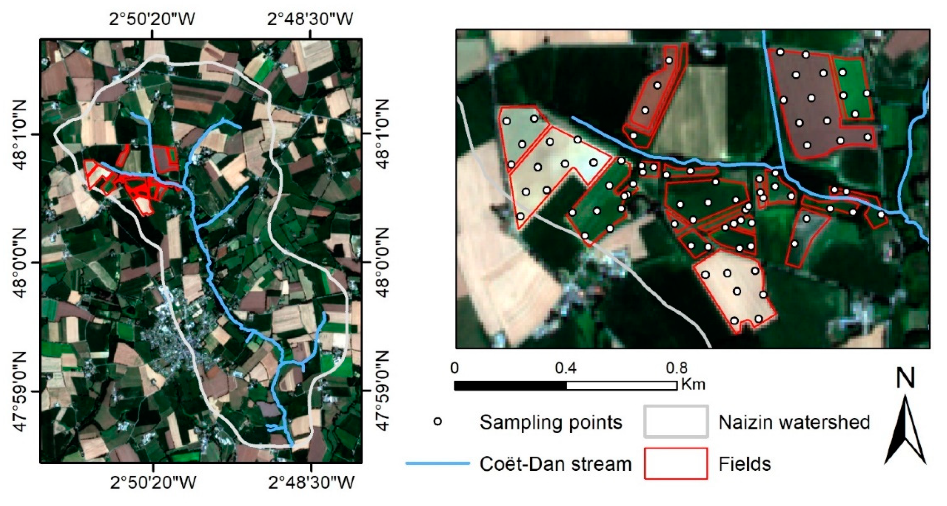
2.1. Study Area and Soil Sampling

The study area is an agricultural land covering ca. 1.5 km2 in the northwestern section (48°0′40′′N, 2°50′40′′W) of the Naizin watershed (western France). The fields studied were located on both sides of a small tributary of the Coët-Dan stream with a moderate slope (<5%). Fields in the northern part have the steepest slopes, with slopes of between 3% and 5%, while those in the southern part are less than 2%. The climate is temperate, with mean annual rainfall of ca. 909 mm. Agriculture is mainly intensive, with cereals, maize, and grassland as the main land uses in crop rotations. The soils are developed on a silty substrate derived from weathered schists and Quaternary aeolian deposits. The dominant soil types are Luvic Cambisols and Haplic Albeluvisols of silty texture [62,63,64].
We sampled 83 points within 22 fields in October 2020. These sampling points were selected using a 100 m triangular grid, except in small fields, in which points were selected randomly (Figure 1). Within 5 m of each point, 5 subsamples of soil were collected randomly from the top 5 cm and then pooled. The samples were air-dried, sieved to 2 mm, and divided in half by sample quartering: one half was sent to the national INRAE soil analysis laboratory (LAS Arras, France) for soil analysis, while the other was used to measure reflectance spectra under laboratory conditions. The SOC content was measured via dry combustion according to certified method NF ISO 10694 [65].

2.2. Laboratory Reflectance Measurements

Soil spectra were measured under laboratory conditions. The 2 mm sieved soil samples were oven-dried at 40 °C for 24 h. Their spectra were then measured using a full range spectroradiometer (ASD FieldSpec® 3, Malvern Panalytical Ltd., London, UK). For each sample, the instrument was calibrated using the white reference standard (Spectralon®, North Sutton, NH, USA) before scanning the soil four times at different positions with the contact probe. Since the spectrometer is equipped with three different detectors [66], the spectra were splice-corrected using ViewSpecPro software to eliminate signal jumps that can occur when changing detector ranges [67]. The mean of the four reflectance spectra in the 400–2450 nm range was used to maximize the signal-to-noise ratio.

2.3. Sentinel-1 and Sentinel-2 Data Pre-Processing

A time series of 80 Sentinel-2 Level-2A images corresponding to our study area (110 × 110 km tile: T30SNE) and acquired from September 2020 to August 2021 were downloaded from the Theia website “https://www.theia-land.fr/ (accessed on 15 October 2021)”. These data are atmospherically corrected using the MAJA processing chain [68] and correspond to ortho-rectified surface reflectance. They cover 10 bands ranging from visible to near-infrared wavelengths and are provided with a mask for clouds and their shadows [69].
After applying the cloud mask, we selected the 26 images with low cloud cover (≤5%) for our study area. We then resampled bands with 20 m spatial resolution to 10 m using the nearest-neighbor assignment method. Following analysis of NDVI profiles, the reflectance of bare soil was extracted using an NDVI threshold [29,70,71]. Pixels with an NDVI <0.25 were considered as bare soils. Only 58 of the 83 sampling points were bare soils on at least one date during the 2020–2021 agricultural season.
The dual-satellite constellation of Sentinel-1A and Sentinel-1B was launched in April 2014 and April 2016, respectively. It provides C-band (frequency = 5.4 GHz) SAR images with a revisit time of 6 days in dual-polarization VV (vertical-vertical) and VH (vertical-horizontal) modes. In this study, we used Level-1 ground-range-detected products acquired from September 2020 to August 2021. Sentinel-1 images were downloaded using the Google Earth Engine application, which provides radar signal images processed for thermal noise removal, radiometric calibration, terrain correction, and speckle filtering.

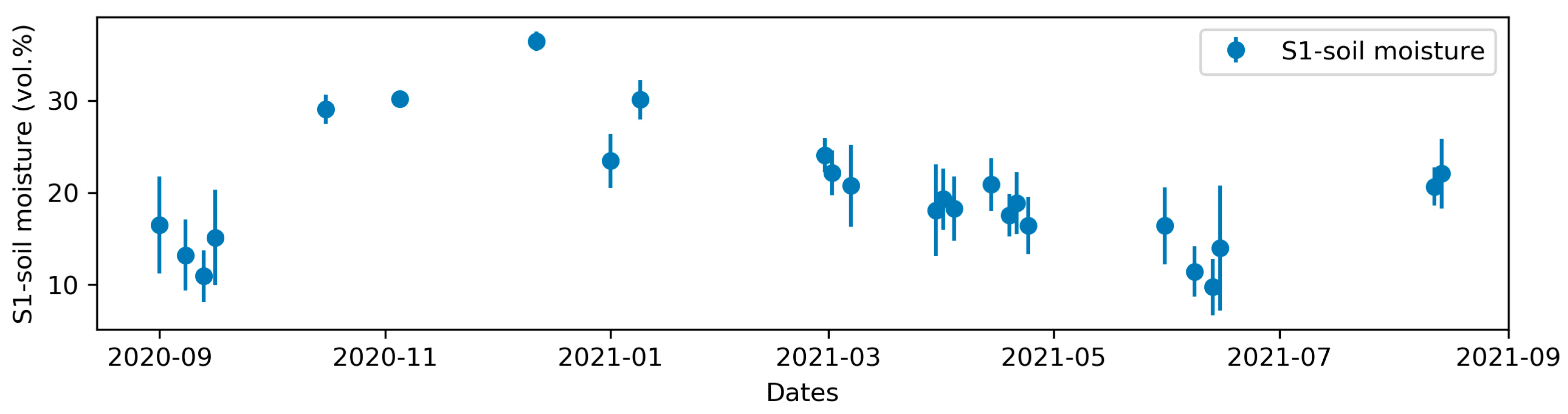
2.4. Sentinel-1 Soil Moisture and Indices Retrieval

From the downloaded Sentinel-1 time series we extracted the radar signal corresponding to bare soils and calculated three radar indices (S1-indices) from its two polarizations (Table 1). For each sampling point, the radar signal was averaged over its corresponding polygon of Thiessen, in the linear scale, then converted to the logarithmic scale and used for S1-indices calculation. If the Sentinel-1 image was acquired on the same date as a Sentinel-2 image, we automatically used it. If not, we calculated the mean radar signal of the two closest dates before and after the Sentinel-2 visit, with an interval not exceeding two days. If only one date was available in the two-day interval, either before or after the Sentinel-2 visit, we used it. In addition, we used estimates of volumetric soil moisture (%) derived from the Sentinel-1 time series (S1-soil moisture) using the approach of El Hajj et al. [72] and validated for our study area by Zayani et al. [73].

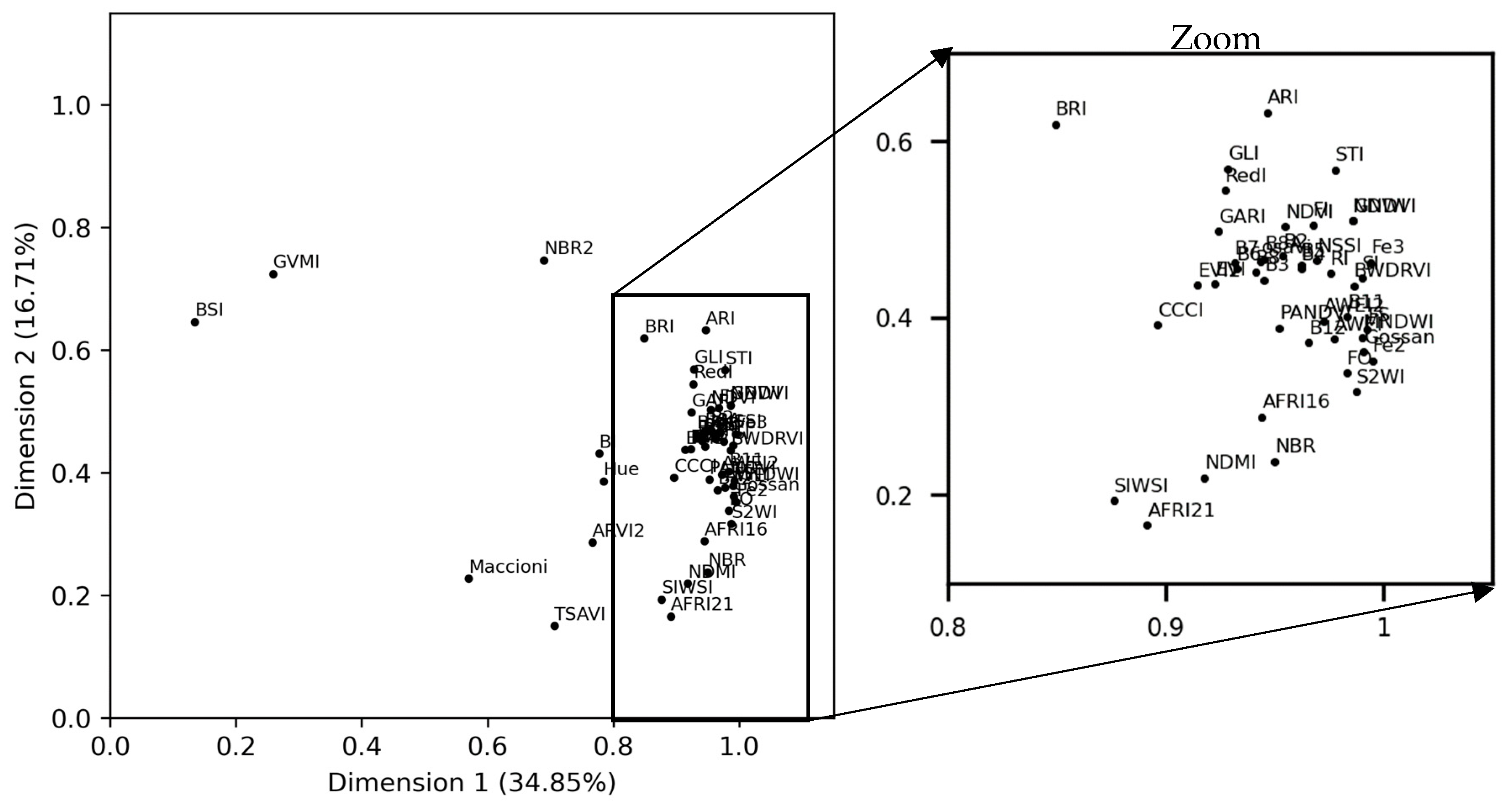
2.5. Retrieval and Analysis of Spectral Indices

In addition to the spectral bands, spectral indices have been developed and used to analyze remote sensing images. These indices are calculated using common equations and enhance some spectral features by minimizing effects of illumination and reducing noise [76,77]. In this study, we used the bare-soil reflectance extracted from the Sentinel-2 images to calculate 40 spectral indices (Appendix A). Based on their application in previous studies, these indices can be grouped into four categories: vegetation, soil, geology, and water. To identify the indices that improved detection of soil variability in space and time, we performed multiple factor analysis (MFA) of the time series of indices for the 58 points of bare soil. This multivariate method, MFA [78] is based on principal component analysis (PCA) and used to summarize data described by several sets of variables organized into groups. Variables of the same group are normalized with a weight equal to the inverse of the first eigenvalue of the PCA, and each variable of the group has its own weight. In our study, each time series of indices was considered as a group. We selected twelve indices that contributed differently to the first two dimensions of the MFA in order to use them to calibrate the models (S2-indices) (Table 2). We then calculated the same 12 indices using the soil spectra measured in the laboratory and the central wavelengths of the Sentinel-2 bands (Lab-indices). To decrease the number of indices potentially included in the prediction models, we selected optimal indices that had the highest Pearson correlation coefficients with SOC content.

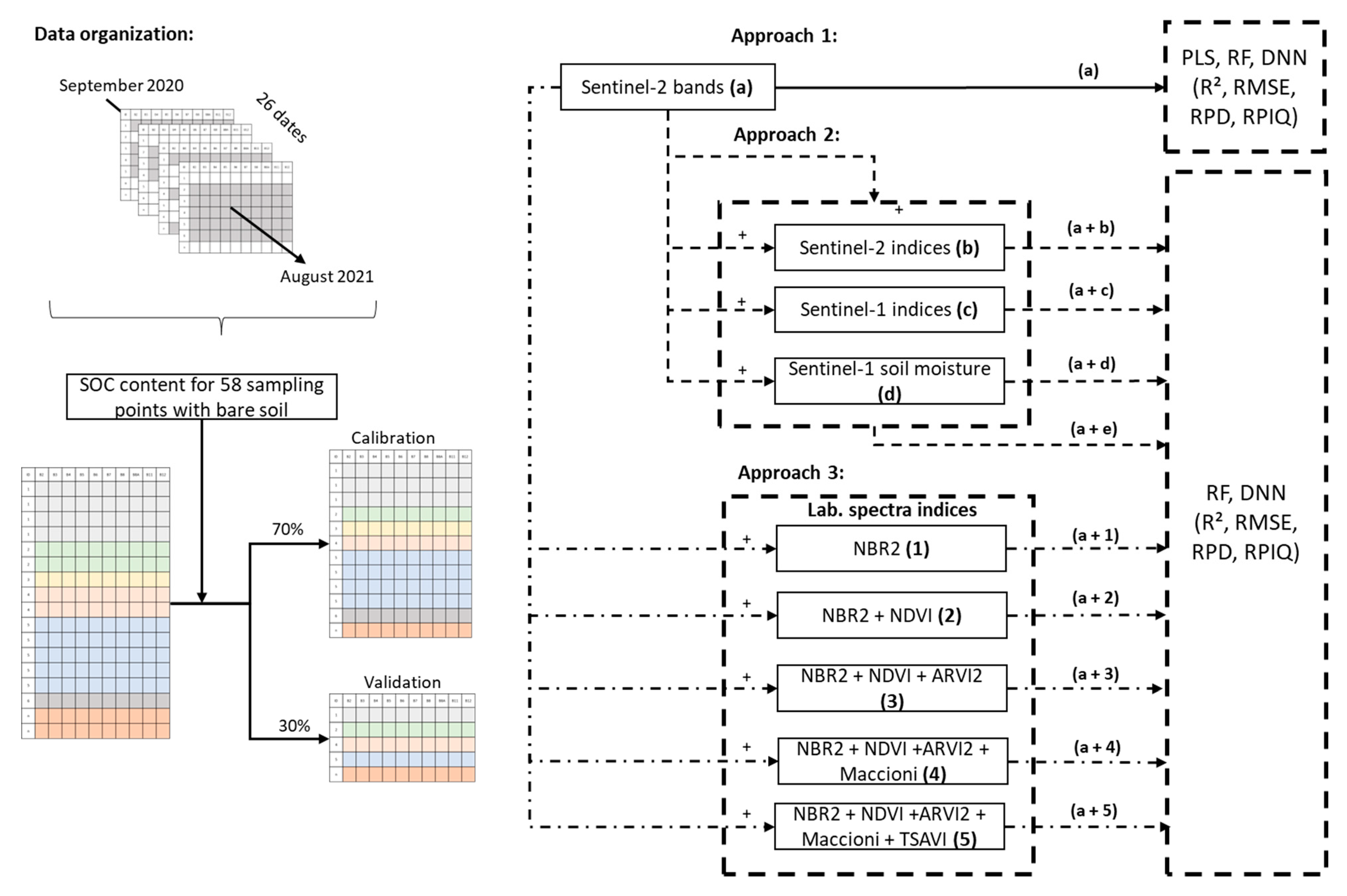
2.6. Prediction Models and Accuracy Assessment

Models were calibrated using three approaches (Figure 2). In the first, only S2 bands (a) were used for model calibration to compare the performance of PLS regression, RF, and the DNN. Based on the results of approach 1, only the two algorithms with the best prediction performance in cross-validation were retained for use in the following two approaches. In the second approach, S2-indices (a + b), S1-indices (a + c), and S1-soil moisture (a + d) were used separately during calibration to assess their individual effects and then used together (a + e). In the third approach, the Lab-indices were added incrementally in the order of decreasing correlation with SOC content (NBR2, NDVI, ARVI2, Maccioni, and TSAVI) to assess their effects on model accuracy. To group all available Sentinel-2 data with bare soil, we constructed a table with 512 rows, which corresponded to “point × date” individuals for the 58 sampling points that had bare soil (range: 1–18 dates). We then randomly split the data into calibration (70%) and validation (30%) datasets. To test the robustness of our approaches, we performed three iterations of each.

2.6.1. Partial Least Squares Regression

PLS regression is the most common linear regression used to predict soil properties. Developed by Wold [92], it maximizes the variance of spectral variables by reducing the original dimension of the spectra into latent variables. It extracts useful components that are strongly correlated with the dependent variables and overcomes problems of multicollinearity between spectral variables [93]. PLS regression performs better than other linear regression methods because of the stability of its latent variables. However, it is sensitive to outliers in the dataset [94] and forces predictions towards the center of the calibration dataset. Thus, for samples with high leverage, prediction uncertainty increases [95]. Non-linear iterative PLS (NIPALS) and statistically inspired modified PLS are the two most common optimization algorithms of PLS regression. In this study, we used the NIPALS algorithm implemented in the scikit-learn 1.0.2 package (Python 3.7.4), which aims to linearize models that have non-linear parameters [92,96]. The optimal number of components was selected using both the coefficient of determination (R2) and the RMSE of a 5-fold cross-validation (RMSECV) and relying on the grid search method (Table A2 in Appendix B). This method allows models parameters to be adjusted by searching a grid of all possible combinations and evaluating them using cross-validation (Figure 3) [97,98].

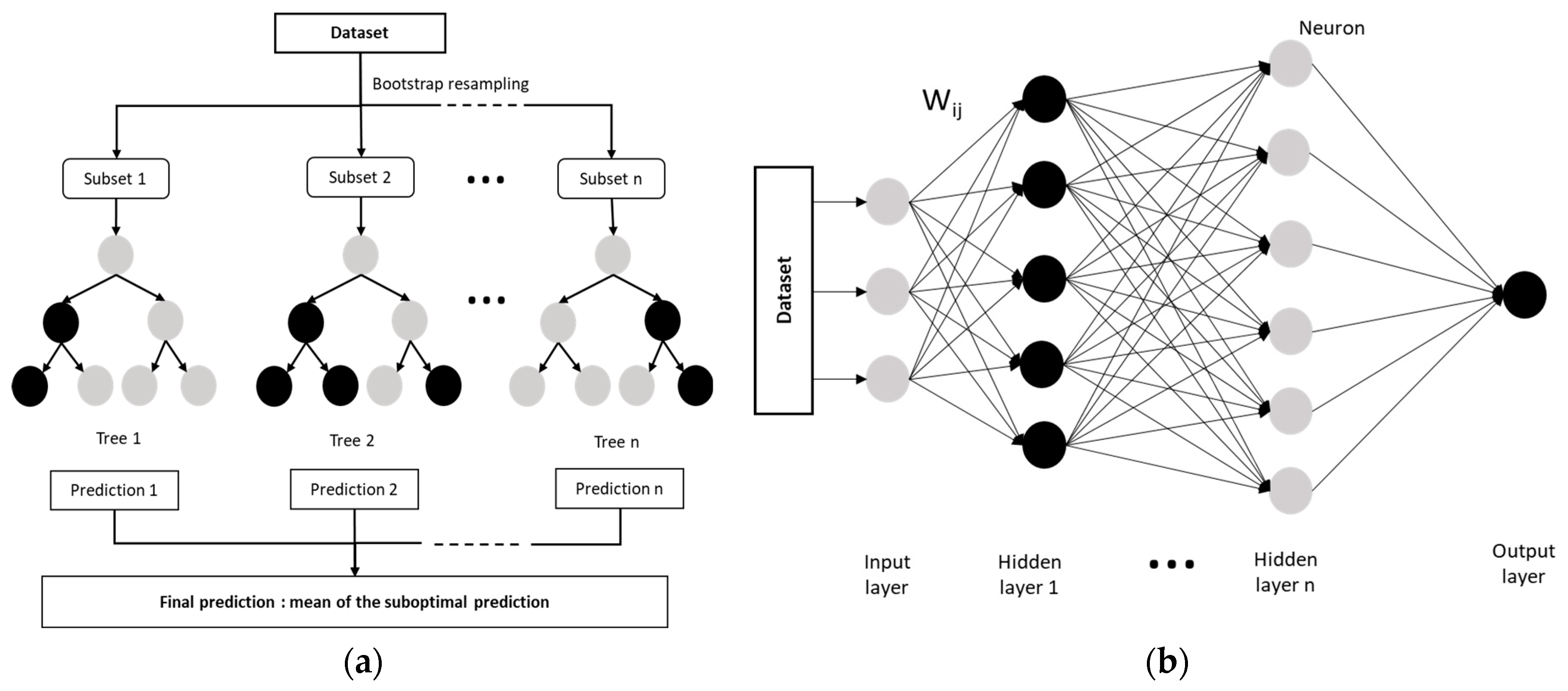
2.6.2. Random Forest

The RF is an ensemble of randomized classification and regression trees that generates multiple decision trees from a randomly selected subset of training samples and uses averaging to increase prediction performance and control overfitting [100]. Many individual trees are trained from bootstrapped subsets of the data, which results in individual learning algorithms being run (Figure 4a). The final prediction equals the mean of these suboptimal trees. The number of trees (n_estimators), the maximum depth of the trees (max_depth), and the number of samples used in each node are user-defined parameters that influence the prediction performance and model efficiency. For example, if the n_estimators value is too large, it will affect the model computation; if it is too small, the model error will not stabilize [101,102]. A higher number of samples used in each node helps to prevent overfitting by avoiding more specific trees [102]. Like other machine-learning algorithms, RF is increasingly used to predict soil properties. It has been shown to increase prediction performance due to its excellent non-linear learning ability and flexibility. In this study, optimal hyperparameters (max_features and max_depth corresponding to the number of features to consider when looking for the best split and the maximum depth of the tree, respectively) were adjusted based on the RMSECV using the “RandomizedSearchCV” and “RandomForestRegressor” functions implemented in the scikit-learn 1.0.2 package (Python 3.7.4) (Table A2 and Table A5 in Appendix B). Randomized search is an alternative method to the grid search method and it performs a random search for hyperparameters within a predefined grid. A fixed number of iterations is performed, and at each iteration the algorithm selects a combination of hyperparameters, tunes the model, and evaluates its performance using RMSECV [97]. The number of trees was fixed at 500 and the number of iterations at 100 for all RF models.

2.6.3. Deep Neural Networks

Neural networks consist of layers of artificial neurons (also called “perceptrons” or “nodes”) that include an input layer, one or more hidden layers, and an output layer. Each node is connected to another and has an associated weight and threshold. It, thus, combines inputs with a set of coefficients that either amplify or dampen that input. An activation function then determines whether and to what extent that signal should progress further through the network to influence the result. Depending on the nature of the problem studied, neural network architectures can be classified by the number and type of layers used, and the number of nodes, or simply as supervised vs. unsupervised learning networks [103,104]. Among the architectures used to predict soil properties [59,105,106], we used a DNN, which has at least two fully connected hidden layers between the input and output layers and provides linear and non-linear relationships between the response variable and a set of predictor variables (Figure 4b) [103]. It was better suited to our case study than a CNN, which is more adapted to data with spatial structure and most commonly used in remote sensing [107]. Thus, the abundant cloud cover over our study area led to a loss of spatial and temporal information. The rectified linear unit (ReLU) activation function was used to establish relationships between input and output neurons in each hidden layer. The optimal number of hidden layers and neurons in each layer was selected based on the RSME using the “tuner.search” framework implemented in the keras_tuner 1.1.3 package (Python 3.8.16) (Table A2 and Table A5 in Appendix B), which is a scalable hyperparameter optimization framework. It is based on Bayesian optimization, Hyperband, and random search algorithms [108]. The random search strategy was used in our case. It consists of a random selection of hyperparameter combinations according to a defined number of iterations, during which the model is trained for a certain number of epochs. As a result, the algorithm returns the best hyperparameters, corresponding to the combination that gave the best performance [97,108]. In our case, the maximum number of iterations was set to 50 (max_trials = 50), the learning rate to 0.01, and the number of epochs to 50.

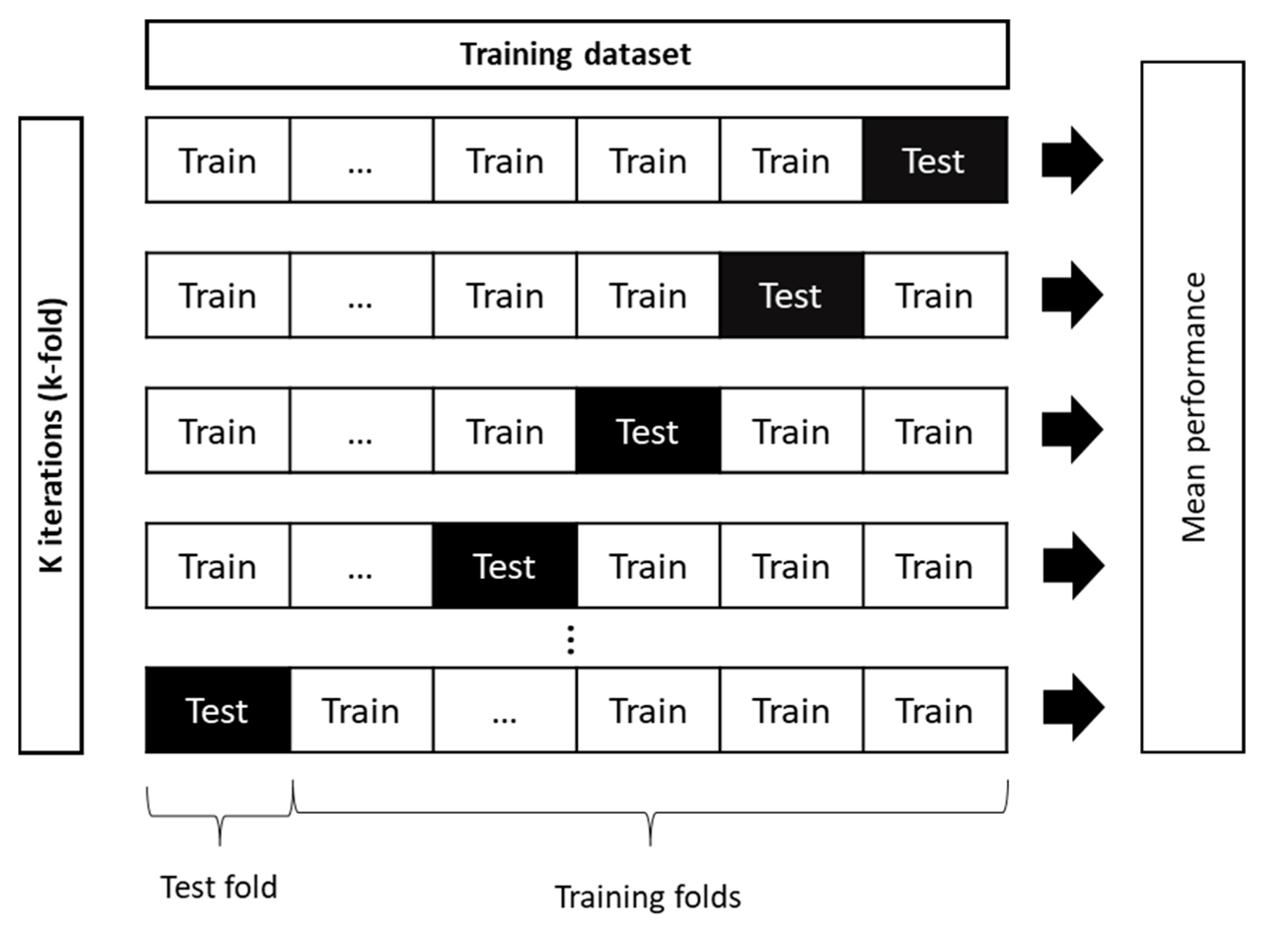
2.6.4. Model Accuracy

The prediction performance of models was evaluated using R2, RMSE, the ratio of performance to deviation (RPD), and the ratio of performance to the interquartile distance (RPIQ) developed by Bellon-Maurel et al. [86]. Higher R2 and lower RMSE indicate a higher model prediction accuracy. As suggested by Chang et al. [109], predictions of soil property models were considered poor for RPD < 1.4, moderate for 1.4 < RPD < 2, and accurate for RPD > 2. Similarly, Nawar and Mouazen [110] considered model predictions very poor for RPIQ < 1.4, fair for 1.4 < RPIQ < 1.7, good for 1.7 < RPIQ < 2, very good for 2 < RPIQ < 2.5, and excellent for RPIQ > 2.5. The formulas for the performance parameters are as follows:
R 2 = i = 1 n y ^ i     y ¯ ² i = 1 n y i     y ¯ ² ,
R M S E = i = 1 n y ^ i     y i ² n ,
R P D = S T D R M S E ,
R P I Q = Q 3     Q 1 R M S E
where y i indicates the measured value of SOC content of the iith sample, y ^ i the predicted value of SOC content of the iith sample, y ¯ the average value of measured SOC content, n the number of samples, (i = 1, 2, 3, …, n), and Q 3     Q 1 indicates the interquartile distance. Q 3 is the value below which we find 75% of the samples and Q 1 is the value below which we find 25% of the samples.

3. Results

3.1. Data Description and Analysis

3.1.1. Descriptive Statistics of Measured SOC Content

The measured SOC contents of the 58 sampling points that were in bare soil, ranged from 15.2–49.4 g·kg−1, with a mean of 22.3 g·kg−1 (Table 3). They lay within the range of SOC content usually observed in the Naizin watershed and were consistent with those measured in a previous study [111]. The descriptive statistics of the calibration and validation datasets generated for the three iterations using the S2 time series are presented in Table 4.

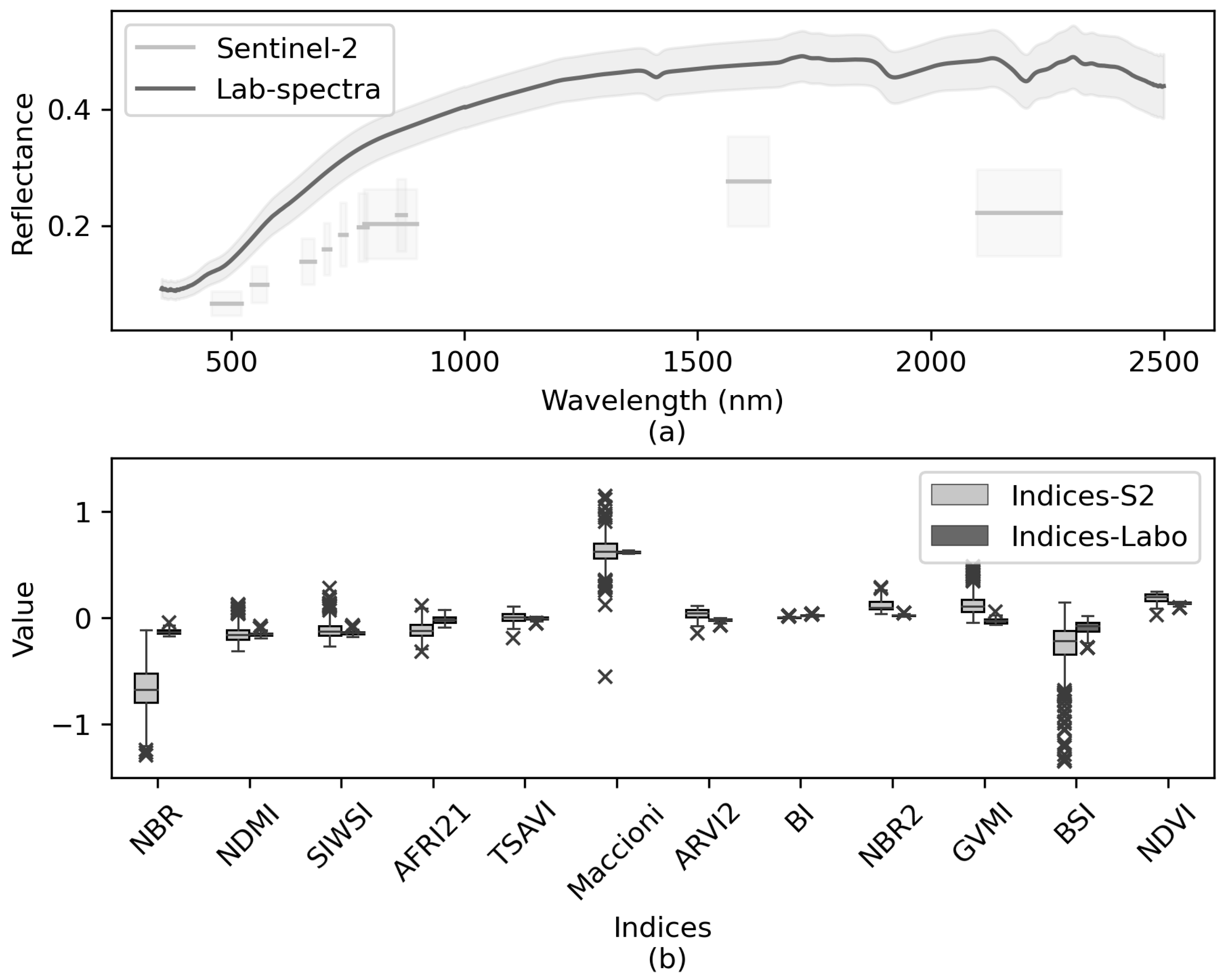
3.1.2. Sentinel-2 and Laboratory Spectral and Sentinel-1 Soil Moisture Information Analysis

The mean reflectance of soil samples was lower for Sentinel-2 spectra than for laboratory spectra (Figure 5a). Some mean S2-indices were lower than mean Lab-indices, while others were higher or nearly the same (Figure 5b). As expected, the former also varied more, since surface conditions, especially soil moisture, varied among sampling points and dates. Some S2-indices (e.g., NBR, BSI) were more sensitive (i.e., variable) than the others. The same was true for Lab-indices, although this variability seemed to be non-significant.
The S2-indices explained more than 51% of total inertia on the first two dimensions of the MFA (Figure 6). Most S2-indices contributed to approximately the same degree (>0.75) to dimension 1 but contributed to varying degrees (0.10–0.75) to dimension 2. Indices BSI and GVMI contributed the least to dimension 1 and among the most to dimension 2.
Most correlations between the Lab-indices and SOC content were significant at p < 0.01 and had absolute values greater than 0.40 (Table 5). Weaker correlations between the Lab-indices and SOC content (r = 0.20–0.30) were significant only at p < 0.05. Indices with r > 0.70 with SOC content were calculated using wavelengths of 665–832 nm, except for NBR2, which used wavelengths of 1614–2202 nm.
S1-soil moisture varied more than the S1-indices (Figure 7). The mean S1-soil moisture varied from 9.8% to36.5%, with standard deviations of 0.8–6.8% that were lowest on the dates with the highest soil moisture (≥30%).

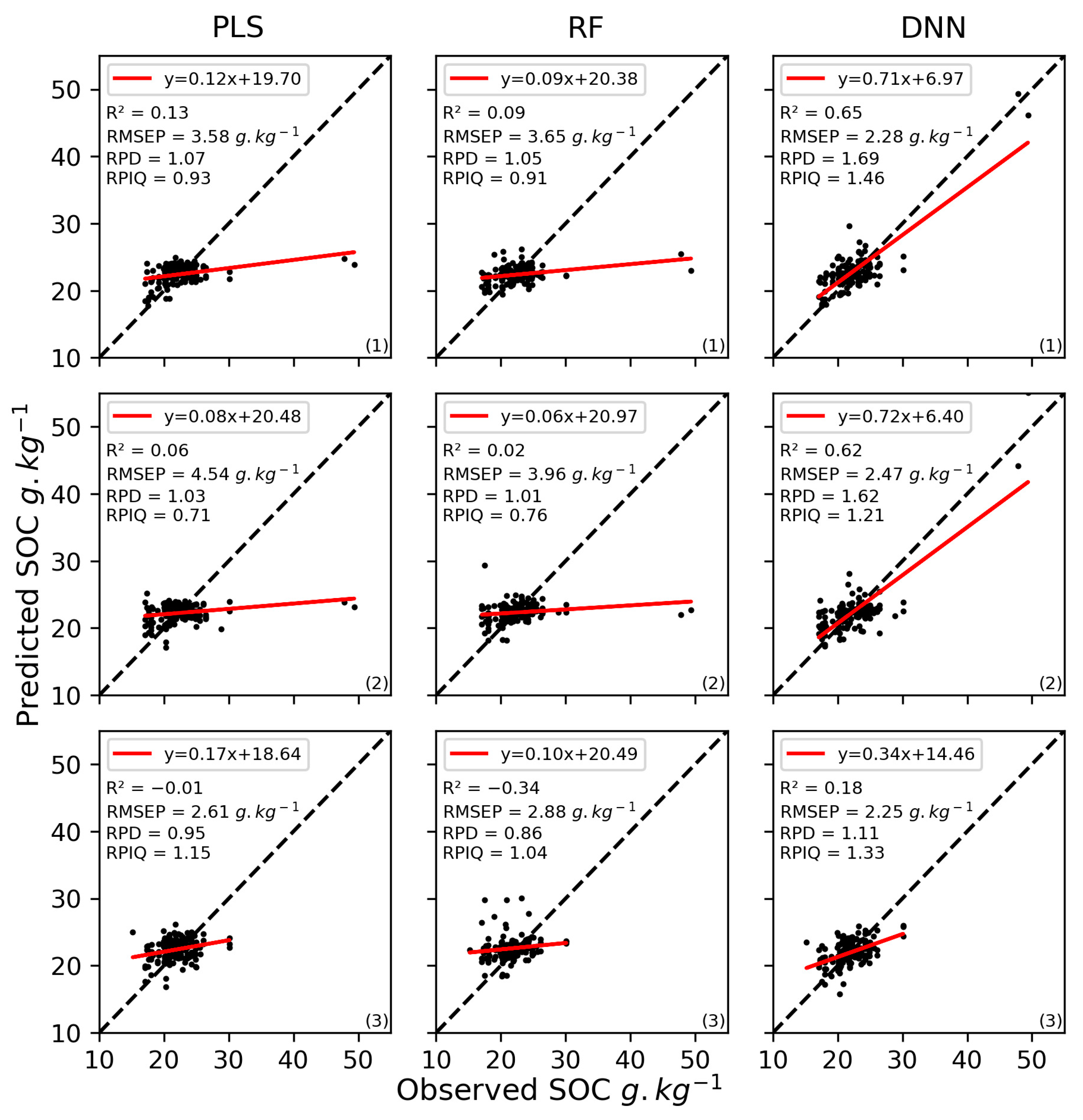
3.2. Model Performance and Comparison

3.2.1. Sentinel-2 Bands Prediction Performance

The results of the validation of the SOC content models using only the Sentinel-2 bands varied among the algorithms (Figure 8, Table A3 in Appendix B) but were relatively stable among the three iterations, with RMSEP equal to 3.57 (±0.79), 3.51 (±0.45), 2.33 (±0.1), for PLS, RF, and DNN, respectively. However, according to R2, the third iteration always produce results of poor quality. Based on the RPD, only models calibrated using DNN performed moderately well in predicting SOC content (1.47 (±0.26)). But, based on the RPIQ, SOC predictions were very poor for the three algorithms (0.93 (±0.18), 0.90 (±0.11), and 1.31 (±0.08)).

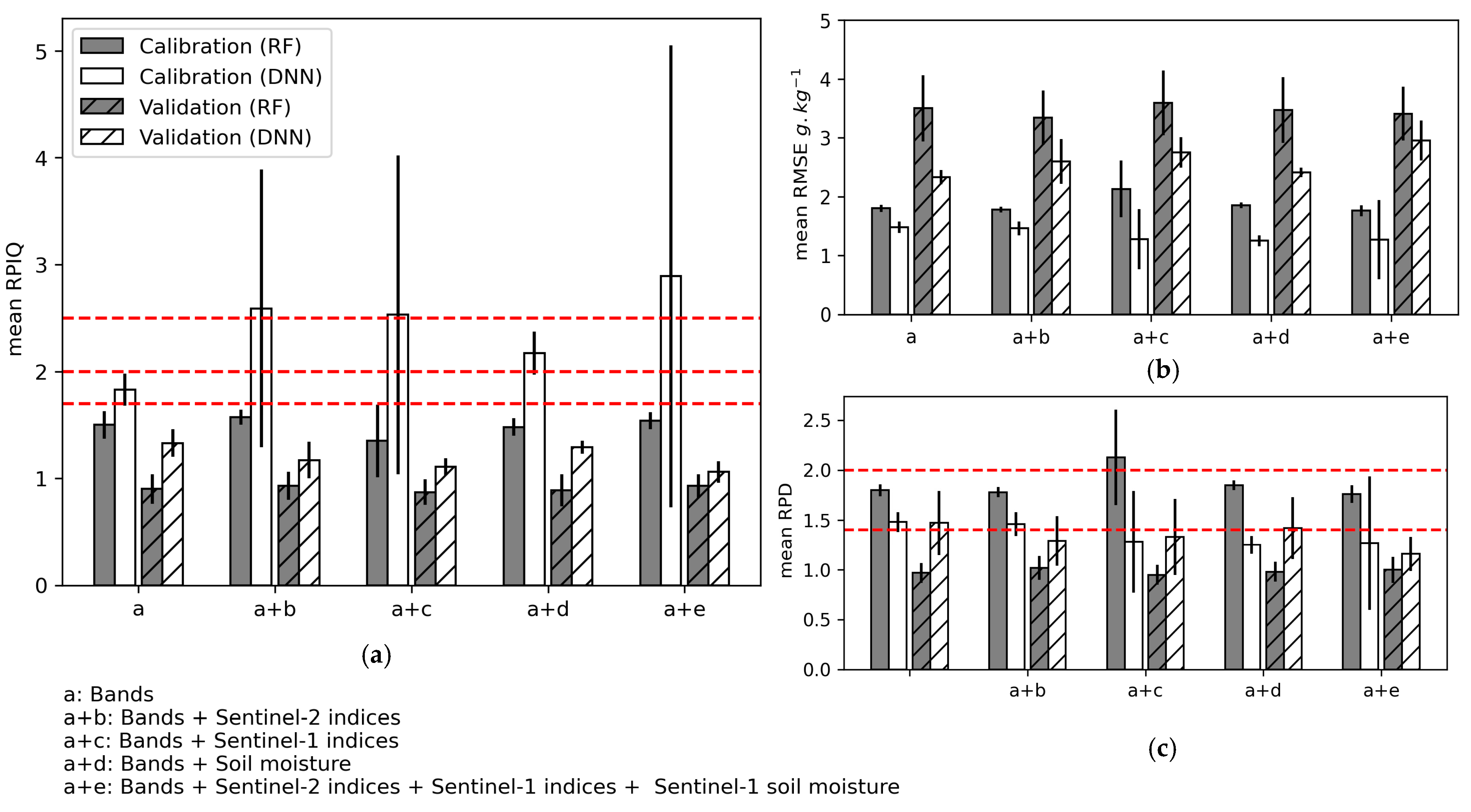
3.2.2. Prediction Performance of Sentinel-2 Bands Combined with Sentinel-2 and Sentinel-1 Indices and Sentinel-1 Soil Moisture

Including the S1- and S2-indices and S1-soil moisture along with the Sentinel-2 bands in the models influenced calibration performance more than validation and the DNN algorithm performance more than the RF algorithm (Figure 9, Table A4 (Appendix B)). Using the DNN, the combination of S2-indices, S1-indices, and S2-indices + S1-indices + S1-soil moisture with Sentinel-2 bands increased the calibration performance the most (mean RPIQ = 2.59 (±1.30), 2.53 (±1.50), and 2.89 (±2.16), respectively), but this result was not stable among the three iterations. Model calibration performance was most stable when S1-soil moisture was included for DNN and RF (mean RPIQ = 2.17 (±0.2) and 1.48 (±0.08), respectively), but doing so had no strong effect on model validation performance. Thus, for all calibrated models, the RPIQ for model validation was always lower than the RPIQ threshold 1.7 considered for accurate predictions. Based on the mean RPD values, only the DNN model calibrated using S2 bands + S1-soil moisture showed a moderate validation performance of SOC prediction (mean RPD = 1.42 (±0.31)), but no improvement was observed compared to using only S2 bands (mean RPD = 1.47 (±0.32)). Mean RMSEP values ranged from 3.34 (±0.46) to 3.59 (±0.55) for RF and from 2.33 (±0.12) to 2.95 (±0.34) for DNN.

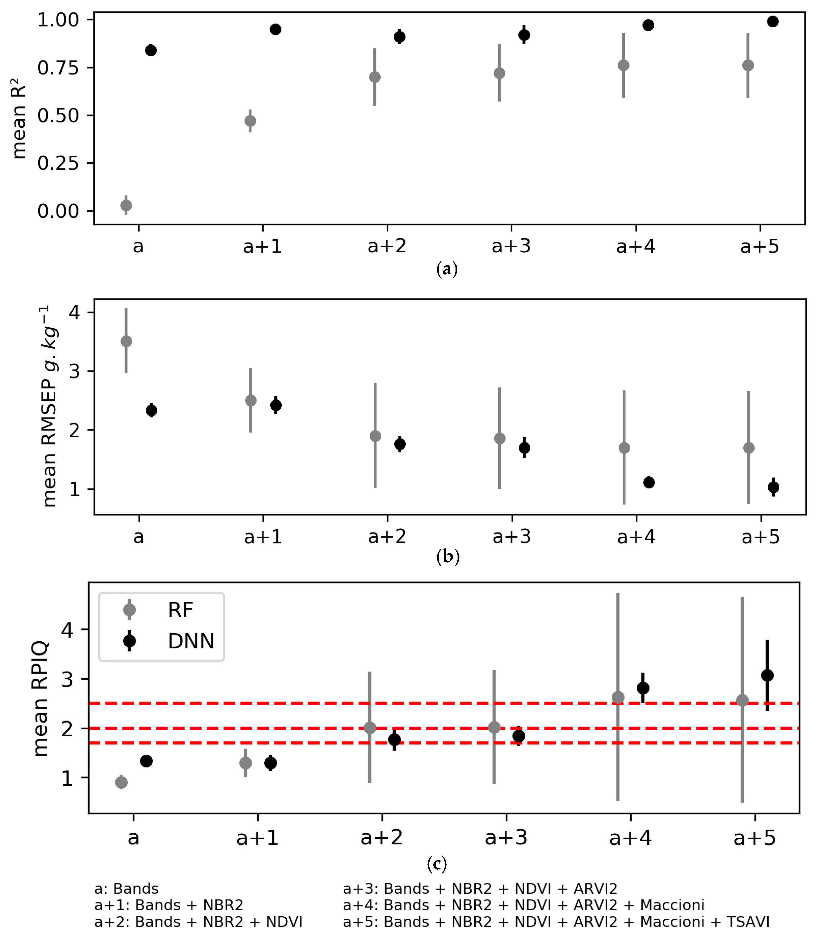
3.2.3. Prediction Performance of Sentinel-2 Bands Combined with Laboratory Spectral Indices

Combining laboratory spectral indices with the Sentinel-2 bands to calibrate models to predict SOC content influenced model performance strongly (Figure 10, Table A6 (Appendix B)). For both the RF and DNN algorithms, the validation criteria with mean RPIQ > 1.7 were obtained when including at least the two indices most correlated with SOC content (i.e., NBR2 and NDVI). However, doing so generated high variability in validation performance for the RF models (i.e., standard deviations of RPIQ of 1.13–2.10), while the validation performance of the DNN models remained relatively stable (mean RPIQ of 1.84 (±0.21) to 3.07 (±0.72)).

4. Discussion

4.1. Factors That Influenced Sentinel-2 Soil Surface Reflectance Spectra

The lower reflectance obtained by Sentinel-2 was observed in most previous studies [33,61] and is related to the acquisition conditions: in particular, atmospheric water, soil moisture, and soil roughness. These parameters strongly influence the energy that is reflected and emitted, which reduces reflectance over the entire spectrum [15,17,112] compared to the laboratory spectra acquired after samples were air-dried, sieved to 2 mm, and oven-dried for 24 h. The variability in this information resulted from the diversity of soils and differences in acquisition conditions among dates, since Sentinel-2 reflectance depends on soil complexity, soil surface conditions, and acquisition conditions. To retrieve the relevant information in the images, all Sentinel-2 spectra that corresponded to bare soil for each sample were grouped in a single table, which can provide an alternative to the mosaicking approaches developed in previous studies [28,38,113]. Vaudour et al. [38] found that temporal mosaicking approaches increased the predicted area but did not predict SOC content better than single-date models. This is because soil conditions, such as soil moisture, soil roughness, and vegetation significantly influence prediction performance by disturbing soil reflectance [31]. Considering Sentinel-2 images acquired on different dates allows one to assess the ability of models to represent different soil conditions and, thus, increase the number and composition of training sample datasets.

4.2. Performance of Calibrated Models Using Only Sentinel-2 Bands: DNN vs. PLS and RF

When using only Sentinel-2 bands, calibrated DNN models outperformed PLS and RF models for all three iterations. These results are consistent with previous studies that found that DNN models are more suitable for predicting SOC due to their ability to capture complex relationships through multiple hidden layers and neurons [61,105,107]. In addition, DNN models can model complex data. For example, Odebiri et al. [105] found that a DNN model improved the prediction of SOC at the national scale, even when using a dataset with high spatial uncertainty (i.e., multiple scales of variation, different sampling sources, and different acquisition dates). Moreover, DNN models in the present study were less sensitive to high-leverage samples (Figure 8) than PLS and RF models were. The low performance of the PLS regression was expected since PLS models are sensitive to highly leveraged samples, which are generally considered as outliers [114]. Although RF models showed RMSEcv of 1.73–1.85 g·kg−1 and fair RPIQ values (RPIQ = 1.41–1.53), validation performance was very poor (RMSEP = 3.51 g·kg−1 (±0.45) and RPIQ = 0.90 (±0.11)). Thus, several studies have found that RF predicted better than other machine-learning techniques, but others have found that the performance of RF classifiers was sensitive to training samples and data dimensions [115]. Compared to the study of Biney et al. [35], our DNN models (R2 = 0.18–0.65 and RPIQ = 1.21–1.46) outperformed their PLS, SVM, CR, and ensemble models developed at the field scale (R2 = 0.11–0.27 and RPIQ = 1.22–1.31). Our models yielded RMSEP of 2.33 g·kg−1 (±0.1), which is better than those obtained by Dvorakova et al. (2023) [116], RMSE = 3.5 g·kg−1 (±0.3), for SOC content ranging from 7.2 to 14.2 g·kg−1 and Vaudour et al. (2021) [38], and RMSE = 3.02–5.86 g·kg−1 for SOC content ranging from 7.04 to 31.9 g·kg−1, in cross validation.

4.3. Effects of Additional Information on Model Calibration and Validation

Including additional information, in particular S2-indices, S1-indices, and S1-soil moisture, was intended to increase the models’ predictive performance by providing new variables that distinguish the varying soil conditions better on different acquisition dates. This additional information had more influence during calibration than validation and on the DNN models than on the RF models (e.g., when including S2-indices, mean RPIQ improved from 2.02 (±0.15) to 2.59 (±1.30) when calibrating the DNN model and from 1.50 (±0.13) to 1.57 (±0.07) when calibrating the RF model) (Figure 9). It likely had more influence during calibration than validation because the validation dataset contained spectral information acquired on dates when soil surface conditions of the sampling points in the training dataset were unknown. In fact, some of the sampling points were bare soil on only a few dates (e.g., 1–3), while others were bare soil on 5–18 dates, which gave the machine-learning algorithms, especially DNN, more opportunities to learn. This may also explain the instability in performance of calibrated DNN models “a + b”, “a + c”, and “a + e” among the iterations (mean RPIQ = 2.59 (±1.30), 2.53 (±1.49), and 2.89 (±2.16), respectively). Thus, the number of dates retained for each sampling point during model calibration strongly influenced model performance. The additional information may have had stronger effects on the DNN models due to their ability to learn and extract more representative features through their hidden layers and neurons [105,107]. Thus, the validation performance of DNN models that included additional information, varied from 2.41 to 2.95 g·kg−1 for RMSEP and from 1.29 to 1.42 for RPD; however, the performance of RF models was almost stable (RMSEP = 3.34–3.59 g·kg−1 and RPD = 0.95–1.02).

4.4. Utility of Including Sentinel-2 Spectral Indices

The higher variability, in some S2-indices than others (Figure 5), supports the idea that these indices can distinguish soil surface conditions. For example, the NDVI and Maccioni indices, both developed to detect green vegetation [70,82], showed different variation ranges. Since we selected only bare soils, we expected the Maccioni index to vary less than the NDVI, but this was not the case. This supports the assumption that the spectral regions of vegetation indices are sensitive to SOC content [33,117]. Similarly, for NBR and NBR2, which were developed to detect burn severity, NBR varied more than NBR2. Dvorakova et al. [118] and Demattê et al. [119] found that NBR2 was correlated with the presence of crop residues, so they used it with NDVI to select bare soil to predict SOC [18,30,38]. In the present study, performance increased significantly when including S2-indices during calibration but not validation of DNN models. This may have been due to potential variation in correlation between Sentinel-2 bands and their derived S2-indices or the SOC content among dates depending on soil surface conditions. For example, Gholizadeh et al. [33] observed that the correlation between Sentinel-2 spectral information and SOC content or soil texture varied among study areas.

4.5. Utility of Including Sentinel-1-Derived Data

Since radar signals are sensitive to soil surface conditions, especially soil moisture, soil surface roughness, and vegetation [73,120,121], we included indices derived from the VV and VH polarizations of Sentinel-1 radar signals. Although these indices appeared to be sensitive to vegetation dynamics [74,75], they increased the prediction performance of DNN models during calibration but with high variability among the three iterations, which is consistent with results of Nguyen et al. [51] and Wang et al. [27]. The latter found that including radar-derived data with multispectral data in SOC prediction models increased prediction performance. We also included Sentinel-1-derived soil moisture because we found in a previous study [73] that soil moisture had more influence than soil surface roughness in the Naizin watershed on the Sentinel-1 radar signal because of relatively high soil moisture. Consequently, we assumed that including Sentinel-1-derived soil moisture could increase prediction performance by considering the variability in soil moisture among dates and sampling points, especially since our study area is located on both sides of a stream. This approach resulted in the most stable improvement during model calibration and the closest validation performance to that of models calibrated using only S2 bands, which showed the lowest RMSEP (RMSEP = 2.41 (±0.08) and 2.33 (±0.12), respectively), supporting the idea that soil moisture strongly influences the performance of SOC prediction models. Urbina-Salazar et al. [50] found that using Sentinel-2 dates with low soil moisture increased performance of SOC prediction models, but that including soil moisture did not, which was the case for the RF model in our study. Thus, the algorithm used influenced the performance of models calibrated with Sentinel-2 data.
By using all of the complementary information simultaneously, the DNN algorithm was able to extract the most appropriate information for predicting SOC content; thus, this approach provides models with more features, which increases their learning capacity. Wang et al. [27] tested different combinations of Landsat TM- and PALSAR-derived data and found that using six TM bands, six TM-derived indices, and four PALSAR polarizations yielded the best model. In addition, Nguyen et al. [51] found that combining Sentinel-1 C-band dual-polarimetric SAR data and Sentinel-2 optical datasets increased prediction performance.

4.6. Effects of Including Laboratory Spectral Indices

Due to the complex nature of soils, their Vis-NIR spectra aggregate multiple soil chromophore spectral signals [122]. Influenced by many other confounding factors, Sentinel-2 soil reflectance predicted SOC less well than spectra acquired under laboratory conditions [28,33,61]. Thus, as suggested by Ben-Dor et al. [10] and confirmed by Vaudour et al. [32], the predictability of a given soil property using remotely sensed data does not depend solely on the property itself or its spectral behavior as a chromophore. When comparing the performance of Sentinel-2A-derived models for two contrasting agroecosystems, Vaudour et al. [32] found that loading values of the Sentinel-2 bands for a given soil property varied among study areas. Consequently, we included laboratory-acquired soil spectral information, assuming that doing so would provide models with more spectral information about soil properties themselves. In addition, Peng et al. [39] improved maps of predicted SOC content by including geospatial estimates of laboratory soil spectra at 1930 nm. Since spectral indices highlight certain spectral features better, we calculated equivalents of the S2-indices using the soil spectra obtained under laboratory conditions. Similarly, Liu et al. [61] found that these bare soil indices were more accurate in predicting SOC densities than those derived from Sentinel-2 imagery; however, their study relied on a single-date Sentinel-2 image acquired in early winter without describing soil surface conditions. Our results showed strong and significant correlations of these indices with the measured SOC content (Table 5). Furthermore, including these indices sequentially in our models improved the prediction of SOC content. With only two indices, we achieved good performance for both RF and DNN models (mean R2 = 0.70 (±0.15) and 0.91 (±0.04) and mean RPIQ = 2.01 (±1.13), and 1.77 (±0.23), respectively). However, the results were less stable for RF than for DNN, even when including five indices. This is consistent with the idea that RF classifiers can be used to classify multisource remote sensing data, mainly due to their computational speed [115], but the fact that they optimize models using only the input datasets identified as important made them unstable in our study. These results suggest that considering the same spectral information acquired in the laboratory for all dates instead of the Sentinel-2 spectral information, which varies as a function of surface conditions, minimizes the effects of surface conditions and highlights the spectral behavior of the soil property itself.

5. Conclusions

This study assessed a new approach for using a time series of Sentinel-2 data combined with Sentinel-1-derived data and Vis-NIR laboratory spectra to predict the SOC content of agricultural soils and tested predictive models of three different algorithms. To retrieve the relevant information contained in the images, all Sentinel-2 spectra that corresponded to bare soil for each soil sample were grouped into a table, which can provide an alternative to mosaicking approaches. Our results showed the following:
The DNN models outperformed the PLS and RF models and the inclusion of additional information (i.e., S2-indices, S1-indices, and S1-soil moisture) influenced the prediction performance of the DNN models more than that of the RF models.
Although the inclusion of additional information improved prediction performance during model calibration, it did not influence model validation. Furthermore, S1-soil moisture gave the most stable improvement in calibration and the closest validation performance to that of models calibrated using only S2 bands, which had the lowest RMSEP.
As the Lab-indices showed strong and significant correlations with measured SOC content, their incremental addition to the models improved the prediction of SOC content, and the addition of only two indices yielded good performances.
Future research could evaluate the approach developed for study areas that have more available Sentinel-2 data and different soil and climate conditions to assess its potential to be generic. Accordingly, the principal objective of this study was to improve the accuracy of SOC content prediction using Sentinel-2 data, with the ultimate goal of producing highly detailed SOC maps. The availability of these maps will be of great help in the crucial issue of monitoring agricultural soils in relation to agricultural practices.

Author Contributions

Conceptualization, H.Z., Y.F., D.M. and C.W.; methodology, H.Z., Y.F., D.M. and C.W.; software, H.Z.; formal analysis, H.Z., Y.F., D.M. and C.W.; writing—original draft preparation, H.Z.; writing—review and editing, Y.F., D.M., C.W., N.B. and E.V.; visualization, H.Z., Z.K. and Z.L.-C.; supervision, Z.K., Z.L.-C., Y.F., D.M. and C.W.; funding acquisition, E.V., Y.F., Z.K. and Z.L.-C. All authors have read and agreed to the published version of the manuscript.

Funding

This study was supported by the European Union’s Horizon H2020 research and innovation European Joint Programme Cofund on Agricultural Soil Management (EJP-SOIL grant no. 862695) and was carried out in the framework of the STEROPES project of EJP-SOIL. It was also supported by the MELICERTES project (ANR-22-PEAE-0010) of the French National Research Agency, under the France2030 program and the national PEPR “agroécologie et numérique” program, and the French–Tunisian project PHC-Utique IPASS (44324WB/20G093). The lead author was awarded a Ph.D. grant by the Tunisian Republic.

Data Availability Statement

The data presented in this study are available on request from the corresponding author.

Acknowledgments

The authors gratefully acknowledge financial support from Rennes Métropole. We also thank all the technical teams for their strong collaboration and support in performing the ground-truth measurements.

Conflicts of Interest

The authors declare no conflict of interest.

Appendix A

Table A1. Equations for Sentinel-2 spectral indices.
Abbreviation Index EquationReference
Vegetation indices
AFRI16 Aerosol free vegetation index 2.1 B 8 A     0.66   ×   B 11 B 8 A   +   0.66   ×   B 11 [79]
AFRI21 Aerosol free vegetation index 2.1 B 8 A     0.5   ×   B 12 B 8 A   +   0.5   ×   B 12 [79]
ARI Anthocyanin reflectance index 1 B 3     1 B 5 [123]
ARVI2 Atmospherically Resistant vegetation index2   0.18   +   1.17   ×   B 8     B 4 B 8   +   B 4 [80]
BRI Browning reflectance index 1 B 3     1 B 5 B 6 [124]
BWDRVI Blue-wide dynamic range vegetation index 0.1   ×   B 7     B 2 0.1   ×   B 7   +   B 2 [125]
CCCI Canopy chlorophyll content index B 8     B 5 / B 8   +   B 5 B 8     B 4 / B 8   +   B 4 [126]
EVI Enhanced vegetation index 2.5   ×   B 8     B 4 B 8   +   6   ×   B 4     7.5   ×   B 2   +   1 [127]
EVI2 Enhanced vegetation index2 2.4   ×   B 8     B 4 B 8   +   B 4   +   1 [128]
GARI Green atmospherically resistant vegetation index B 8     B 3     B 2     B 4 B 8   +   B 3   +   B 2     B 4 [129]
GLI Green leaf index 2   ×   B 3     B 5     B 2 2   ×   B 3   +   B 5   +   B 2 [130]
GNDVI Green normalized difference vegetation index B 8     B 3 B 8   +   B 3 [129]
GVMI Global vegetation moisture index B 8   +   0.1     B 12   +   0.02 B 8   +   0.1   +   B 12   +   0.02 [81]
Maccioni Maccioni vegetation index B 7     B 5 B 7     B 4 [82]
NBR Normalized burn ratio B 8     B 12 B 8   +   B 12 [83]
NBR2 Normalized burned Ratio 2 B 11     B 12 B 11   +   B 12 [84,85]
NDVI Normalized difference vegetation index B 8     B 4 B 8   +   B 4 [70]
NSSI NPV-soil separation index B 8 A     B 7 B 8 A B 7 [131]
OSAVI Optimized soil-adjusted vegetation index B 8     B 4 B 8   +   B 4   +   0.16 [132]
PANDVI Pan normalized difference vegetation index B 8     B 3   +   B 4   +   B 2 B 8   +   B 3   +   B 4   +   B 2 [133]
SIWSI Shortwave infrared water stress index B 8 A     B 11 B 8 A   +   B 11 [86]
TSAVI Soil-adjusted vegetation index 1.22   ×   ( B 8     1.22     B 4     0.03 ) 1.22   ×   B 8   +   B 4     1.22   ×   0.03   +   0.08   ×   ( 1   +   1.22 2 ) [87]
Soil indices
BI Brightness index B 2 2   +   B 3 2   +   B 4 2 3 [89,134]
BSI Bare soil index B 12     B 4     B 8     B 2 B 12     B 4   +   B 8     B 2 [90]
FI Form index 2   ×   B 4     B 3     B 2 B 3     B 2 [135]
Hue Hue index a r c t a n 2   ×   B 5     B 3     B 2 30.5   ×   B 3     B 5 [135]
RedI Redness index B 4 2 B 3 3 [89]
SI Saturation index B 4     B 2 B 4 [135]
S2WI Soil moisture index B 8     B 11     B 12 B 8   +   B 11   +   B 12 [32]
STI Soil tillage index B 11 B 12 [136]
Geology indices
Fe2 Ferrous iron index B 12 B 8     B 3 B 4 [137]
Fe3 Ferric iron index B 3 B 4 [137]
FO Ferric oxides index B 11 B 8 [137]
FS Ferrous silicates index B 12 B 11 [137]
Gossan Gossan index B 11 B 4 [137]
Water indices
AWEI Automated water extraction index not dominant shadow 4   ×   B 3     B 11     0.25   ×   B 8   +   2.75   ×   B 12 [121]
AWEI2 Automated water extraction index dominant shadow B 2   +   2.5   ×   B 3     1.5   ×   B 8   +   B 1     0.25   ×   B 12 [138]
MNDWI Modified normalized difference water index B 3     B 11 B 3   +   B 11 [139]
NDMI Normalized difference moisture index B 8     B 11 B 8   +   B 11 [91]
NDWI Normalized difference water index B 3     B 8 B 3   +   B 8 [140]

Appendix B

Table A2. Adjusted parameters for models when using only Sentinel-2 bands and when including Sentinel-2 indices, Sentinel-1 indices, and/or Sentinel-1 soil moisture.
Input PLSRFDNN
It.FactorsScaleMax_FeaturesMax_DepthNum_Layers
a(1)6True0.607012
(2)5False auto108
(3)6True0.60707
a + b(1)--0.752010
(2)--0.60305
(3)--0.857012
a + c(1)--0.955012
(2)--0.851011
(3)--0.851012
a + d(1)--0.6None5
(2)--0.85109
(3)--0.60None9
a + e(1)--0.607013
(2)--0.603013
(3)--0.60None13
Table A3. Detailed performance of models calibrated using only Sentinel-2 bands with the partial least squares (PLS) regression, random forest (RF), or deep neural network (DNN) algorithms (Alg.) for the three iterations (It.) ((1), (2), and (3)).
CalibrationValidation
Alg.It.R2RMSECVRPDRPIQr2RMSEPRPDRPIQ
PLS(1)0.153.271.080.790.133.581.070.93
(2)0.153.211.080.830.063.881.030.77
(3)0.173.671.10.77−0.102.610.951.15
RF(1)0.731.821.941.410.093.651.050.91
(2)0.751.732.001.540.023.961.010.76
(3)0.791.852.171.53−0.342.880.861.04
DNN(1)0.811.552.291.670.652.281.691.46
(2)0.851.362.551.960.622.471.621.21
(3)0.861.532.631.860.182.251.111.33
Table A4. Detailed performance for the three iterations (It.) ((1), (2), and (3)) of the calibrated random forest (RF) and deep neural network (DNN) models and their validation when including Sentinel-2 indices, Sentinel-1 indices, and/or Sentinel-1 soil moisture.
RFDNN
CalibrationValidationCalibrationValidation
InputIt.R2RMSECVRPDRPIQr2RMSEPRPDRPIQR2RMSERPDRPIQr2RMSEPRPDRPIQ
a(1)0.731.821.941.410.093.651.050.910.811.552.291.670.652.281.691.46
(2)0.751.732.001.540.023.961.010.760.851.362.551.960.622.471.621.21
(3)0.791.852.171.53−0.342.880.861.040.861.532.631.860.182.251.111.33
a + b(1)0.761.742.031.480.183.471.110.960.861.332.661.940.562.551.511.31
(2)0.721.831.901.460.133.731.070.80.811.532.271.740.433.011.330.99
(3)0.81.782.261.60−0.302.830.881.060.970.705.874.080.022.461.021.22
a + c(1)0.432.671.330.970.043.761.020.890.821.512.351.710.442.871.341.16
(2)0.741.781.961.50−0.024.040.990.740.781.642.111.620.462.931.371.02
(3)0.771.932.081.47−0.442.980.831.000.970.676.024.25−0.112.610.951.14
a + d(1)0.721.871.901.380.093.661.050.910.861.332.671.940.592.471.561.35
(2)0.731.801.931.490.033.921.020.760.891.153.012.320.632.441.641.23
(3)0.781.892.131.51−0.302.840.871.050.91.263.22.260.132.321.071.29
a + e(1)0.751.781.991.450.163.511.090.950.811.562.281.660.313.21.211.04
(2)0.771.662.101.610.093.811.050.780.980.507.015.380.43.081.300.97
(3)0.791.842.181.54−0.372.910.851.030.811.752.31.63−0.062.560.971.17
a: Bands, a + b: Bands + Sentinel-2 indices, a + c: Bands + Sentinel-1 indices, a + d: Bands + Soil moisture, a + e: Bands + Sentinel-2 indices + Sentinel-1 indices + Sentinel-1 soil moisture.
Table A5. Adjusted parameters for models when adding laboratory spectral indices incrementally in the order of decreasing correlation with soil organic carbon content.
Input RFDNN
It.Max_FeaturesMax_DepthNum_Layers
a(1)0.607012
(2)auto108
(3)0.60707
a + 1(1)auto7011
(2)Auto 1010
(3)auto2010
a + 2(1)0.85107
(2)auto306
(3)auto3012
a + 3(1)0.585012
(2)auto3011
(3)auto703
a + 4(1)auto1011
(2)0.95None12
(3)0.95None12
a + 5(1)auto2013
(2)auto309
(3)0.95305
Table A6. Detailed performance for the three iterations (It.) ((1), (2), and (3)) of the calibrated random forest (RF) and deep neural network (DNN) models and their validation when adding laboratory spectral indices incrementally in the order of decreasing correlation with soil organic carbon content.
RFDNN
CalibrationValidationCalibrationValidation
InputIt.R2RMSECVRPDRPIQr2RMSEPRPDRPIQR2RMSERPDRPIQr2RMSEPRPDRPIQ
a(1)0.731.821.941.410.093.651.050.910.731.552.291.670.652.281.691.46
(2)0.751.732.001.540.023.961.010.760.751.362.551.960.622.471.621.21
(3)0.791.852.171.53−0.342.880.861.040.791.532.631.860.182.251.111.33
a + 1(1)0.811.532.321.690.432.891.331.150.960.695.183.760.652.271.71.47
(2)0.821.452.391.840.532.741.461.090.960.675.173.970.592.561.561.17
(3)0.861.502.681.900.441.871.331.600.940.954.232.990.042.431.021.23
a + 2(1)0.831.472.421.760.572.521.521.320.960.695.143.750.821.642.352.03
(2)0.791.582.201.690.672.301.741.300.881.202.912.230.771.922.091.56
(3)0.861.462.741.940.870.882.823.400.901.253.222.270.521.721.451.74
a + 3(1)0.791.612.211.610.582.501.541.33 0.871.272.792.020.81.732.221.92
(2)0.821.452.401.840.702.201.811.360.970.625.604.300.781.862.161.61
(3)0.871.442.791.970.870.892.793.360.921.163.462.440.631.501.661.99
a + 4(1)0.841.412.521.830.612.391.611.390.950.784.543.300.921.103.513.04
(2)0.831.412.461.890.722.111.891.420.990.408.756.720.931.023.922.92
(3)0.881.362.962.060.940.594.215.070.960.814.983.520.761.212.052.46
a + 5(1)0.841.402.531.840.602.421.591.380.990.2116.7412.170.950.854.513.90
(2)0.831.432.421.860.732.081.921.440.990.3410.217.840.921.103.652.72
(3)0.891.323.042.150.940.614.074.900.990.468.656.110.781.152.162.59
a: Bands, a + 1: Bands + NBR2, a + 2: Bands + NBR2 + NDVI, a + 3: Bands + NBR2 + NDVI + ARVI2; a + 4: Bands + NBR2 + NDVI + ARVI2 + Maccioni, a + 5: Bands + NBR2 + NDVI + ARVI2 + Maccioni + TSAVI.

References

  1. Shepherd, M.A.; Harrison, R.; Webb, J. Managing soil organic matter—Implications for soil structure on organic farms. Soil Use Manag. 2002, 18, 284–292. [Google Scholar] [CrossRef]
  2. Kirchmann, H.; Haberhauer, G.; Kandeler, E.; Sessitsch, A.; Gerzabek, M.H. Effects of level and quality of organic matter input on carbon storage and biological activity in soil: Synthesis of a long-term experiment. Glob. Biogeochem. Cycles 2004, 18, 1–9. [Google Scholar] [CrossRef]
  3. Johannes, A.; Sauzet, O.; Matter, A.; Boivin, P. Soil organic carbon content and soil structure quality of clayey cropland soils: A large-scale study in the Swiss Jura region. Soil Use and Management. 2023, 39, 1–10. [Google Scholar] [CrossRef]
  4. Ben-Dor, E. Quantitative remote sensing of soil properties. In Advances in Agronomy; Academic Press, Inc.: Cambridge, MA, USA, 2002; Volume 75, pp. 173–243. ISBN 9780120007936. [Google Scholar]
  5. Stenberg, B.; Viscarra Rossel, R.A.; Mouazen, A.M.; Wetterlind, J. Visible and Near Infrared Spectroscopy in Soil Science. In Advances in Agronomy; Elsevier Inc.: Amsterdam, The Netherlands, 2010; Volume 107, pp. 163–215. [Google Scholar]
  6. Nocita, M.; Stevens, A.; van Wesemael, B.; Aitkenhead, M.; Bachmann, M.; Barthès, B.G.; Ben-Dor, E.; Brown, D.J.; Clairotte, M.; Csorba, A.; et al. Soil Spectroscopy: An Alternative to Wet Chemistry for Soil Monitoring. Adv. Agron. 2015, 132, 139–159. [Google Scholar]
  7. Chabrillat, S.; Ben-Dor, E.; Cierniewski, J.; Gomez, C.; Schmid, T.; van Wesemael, B. Imaging Spectroscopy for Soil Mapping and Monitoring; Surveys in Geophysics; Springer: Dordrecht, The Netherlands, 2019; Volume 40, ISBN 0123456789. [Google Scholar]
  8. Vaudour, E.; Gholizadeh, A.; Castaldi, F.; Saberioon, M.M.; Borůvka, L.; Urbina-Salazar, D.; Fouad, Y.; Arrouays, D.; Richer-de-Forges, A.C.; Biney, J.; et al. Satellite Imagery to Map Topsoil Organic Carbon Content over Cultivated Areas: An Overview. Remote Sens. 2022, 14, 2917. [Google Scholar] [CrossRef]
  9. Francos, N.; Ogen, Y.; Ben-Dor, E. Spectral Assessment of Organic Matter with Different Composition Using Reflectance Spectroscopy. Remote Sens. 2021, 13, 1549. [Google Scholar] [CrossRef]
  10. Ben-Dor, E.; Chabrillat, S.; Demattê, J.A.M.; Taylor, G.R.; Hill, J.; Whiting, M.L.; Sommer, S. Using Imaging Spectroscopy to study soil properties. Remote Sens. Environ. 2009, 113, S38–S55. [Google Scholar] [CrossRef]
  11. Stevens, A.; van Wesemael, B.; Bartholomeus, H.; Rosillon, D.; Tychon, B.; Ben-Dor, E. Laboratory, field and airborne spectroscopy for monitoring organic carbon content in agricultural soils. Geoderma 2008, 144, 395–404. [Google Scholar] [CrossRef]
  12. Angelopoulou, T.; Tziolas, N.; Balafoutis, A.; Zalidis, G.; Bochtis, D. Remote sensing techniques for soil organic carbon estimation: A review. Remote Sens. 2019, 11, 676. [Google Scholar] [CrossRef]
  13. Franceschini, M.H.D.; Demattê, J.A.M.; da Silva Terra, F.; Vicente, L.E.; Bartholomeus, H.; de Souza Filho, C.R. Prediction of soil properties using imaging spectroscopy: Considering fractional vegetation cover to improve accuracy. Int. J. Appl. Earth Obs. Geoinf. 2015, 38, 358–370. [Google Scholar] [CrossRef]
  14. Lagacherie, P.; Baret, F.; Feret, J.B.; Madeira Netto, J.; Robbez-Masson, J.M. Estimation of soil clay and calcium carbonate using laboratory, field and airborne hyperspectral measurements. Remote Sens. Environ. 2008, 112, 825–835. [Google Scholar] [CrossRef]
  15. Denis, A.; Stevens, A.; van Wesemael, B.; Udelhoven, T.; Tychon, B. Soil organic carbon assessment by field and airborne spectrometry in bare croplands: Accounting for soil surface roughness. Geoderma 2014, 226–227, 94–102. [Google Scholar] [CrossRef]
  16. Bogrekci, I.; Lee, W.S. Effects of Soil Moisture Content on Absorbance Spectra of Sandy Soils in Sensing Phosphorus Concentrations Using Uv-Vis-Nir Spectroscopy. Am. Soc. Agric. Biol. Eng. 2006, 49, 1175–1180. [Google Scholar] [CrossRef]
  17. Nocita, M.; Stevens, A.; Noon, C.; Van Wesemael, B. Prediction of soil organic carbon for different levels of soil moisture using Vis-NIR spectroscopy. Geoderma 2013, 199, 37–42. [Google Scholar] [CrossRef]
  18. Castaldi, F.; Chabrillat, S.; Don, A.; van Wesemael, B. Soil organic carbon mapping using LUCAS topsoil database and Sentinel-2 data: An approach to reduce soil moisture and crop residue effects. Remote Sens. 2019, 11, 2121. [Google Scholar] [CrossRef]
  19. Diek, S.; Chabrillat, S.; Nocita, M.; Schaepman, M.E.; de Jong, R. Minimizing soil moisture variations in multi-temporal airborne imaging spectrometer data for digital soil mapping. Geoderma 2019, 337, 607–621. [Google Scholar] [CrossRef]
  20. Brown, D.J.; Shepherd, K.D.; Walsh, M.G.; Dewayne Mays, M.; Reinsch, T.G. Global soil characterization with VNIR diffuse reflectance spectroscopy. Geoderma 2006, 132, 273–290. [Google Scholar] [CrossRef]
  21. Ramirez-Lopez, L.; Behrens, T.; Schmidt, K.; Stevens, A.; Demattê, J.A.M.; Scholten, T. The spectrum-based learner: A new local approach for modeling soil vis-NIR spectra of complex datasets. Geoderma 2013, 195–196, 268–279. [Google Scholar] [CrossRef]
  22. Clairotte, M.; Grinand, C.; Kouakoua, E.; Thébault, A.; Saby, N.P.A.; Bernoux, M.; Barthès, B.G. National calibration of soil organic carbon concentration using diffuse infrared re fl ectance spectroscopy. Geoderma 2016, 276, 41–52. [Google Scholar] [CrossRef]
  23. Gomez, C.; Chevallier, T.; Moulin, P.; Bouferra, I.; Hmaidi, K.; Arrouays, D.; Jolivet, C.; Barthès, B.G. Prediction of soil organic and inorganic carbon concentrations in Tunisian samples by mid-infrared reflectance spectroscopy using a French national library. Geoderma 2020, 375, 114469. [Google Scholar] [CrossRef]
  24. Peng, Y.; Knadel, M.; Gislum, R.; Deng, F.; Norgaard, T.; De Jonge, L.W.; Moldrup, P.; Greve, M.H. Predicting soil organic carbon at field scale using a national soil spectral library. J. Near Infrared Spectrosc. 2013, 21, 213–222. [Google Scholar] [CrossRef]
  25. Cambou, A.; Cardinael, R.; Kouakoua, E.; Villeneuve, M.; Durand, C.; Barthès, B.G. Prediction of soil organic carbon stock using visible and near infrared reflectance spectroscopy (VNIRS) in the field. Geoderma 2016, 261, 151–159. [Google Scholar] [CrossRef]
  26. Bai, Z.; Xie, M.; Hu, B.; Luo, D.; Wan, C.; Peng, J.; Shi, Z. Estimation of Soil Organic Carbon Using Vis-NIR Spectral Data and Spectral Feature Bands Selection in Southern Xinjiang, China. Sensors 2022, 22, 6124. [Google Scholar] [CrossRef] [PubMed]
  27. Wang, X.; Zhang, Y.; Atkinson, P.M.; Yao, H. Predicting soil organic carbon content in Spain by combining Landsat TM and ALOS PALSAR images. Int. J. Appl. Earth Obs. Geoinf. 2020, 92, 102182. [Google Scholar] [CrossRef]
  28. Castaldi, F. Sentinel-2 and Landsat-8 multi-temporal series to estimate topsoil properties on croplands. Remote Sens. 2021, 13, 3345. [Google Scholar] [CrossRef]
  29. Castaldi, F.; Hueni, A.; Chabrillat, S.; Ward, K.; Buttafuoco, G.; Bomans, B.; Vreys, K.; Brell, M.; van Wesemael, B. Evaluating the capability of the Sentinel 2 data for soil organic carbon prediction in croplands. ISPRS J. Photogramm. Remote Sens. 2019, 147, 267–282. [Google Scholar] [CrossRef]
  30. Dvorakova, K.; Heiden, U.; Van Wesemael, B. Sentinel-2 exposed soil composite for soil organic carbon prediction. Remote Sens. 2021, 13, 1791. [Google Scholar] [CrossRef]
  31. Vaudour, E.; Gomez, C.; Loiseau, T.; Baghdadi, N.; Loubet, B.; Arrouays, D.; Ali, L.; Lagacherie, P. The impact of acquisition date on the prediction performance of topsoil organic carbon from Sentinel-2 for croplands. Remote Sens. 2019, 11, 2143. [Google Scholar] [CrossRef]
  32. Vaudour, E.; Gomez, C.; Fouad, Y.; Lagacherie, P. Sentinel-2 image capacities to predict common topsoil properties of temperate and Mediterranean agroecosystems. Remote Sens. Environ. 2019, 223, 21–33. [Google Scholar] [CrossRef]
  33. Gholizadeh, A.; Žižala, D.; Saberioon, M.M.; Borůvka, L. Soil organic carbon and texture retrieving and mapping using proximal, airborne and Sentinel-2 spectral imaging. Remote Sens. Environ. 2018, 218, 89–103. [Google Scholar] [CrossRef]
  34. Žižala, D.; Minarík, R.; Zádorová, T. Soil organic carbon mapping using multispectral remote sensing data: Prediction ability of data with different spatial and spectral resolutions. Remote Sens. 2019, 11, 2947. [Google Scholar] [CrossRef]
  35. Biney, J.K.M.; Vašát, R.; Bell, S.M.; Kebonye, N.M.; Klement, A.; John, K.; Borůvka, L. Prediction of topsoil organic carbon content with Sentinel-2 imagery and spectroscopic measurements under different conditions using an ensemble model approach with multiple pre-treatment combinations. Soil Tillage Res. 2022, 220, 105379. [Google Scholar] [CrossRef]
  36. Gholizadeh, A.; Saberioon, M.M.; Viscarra Rossel, R.A.; Borůvka, L.; Klement, A. Spectroscopic measurements and imaging of soil colour for field scale estimation of soil organic carbon. Geoderma 2020, 357, 113972. [Google Scholar] [CrossRef]
  37. Matinfar, H.R.; Maghsodi, Z.; Mousavi, S.R.; Rahmani, A. Evaluation and Prediction of Topsoil organic carbon using Machine learning and hybrid models at a Field-scale. Catena 2021, 202, 105258. [Google Scholar] [CrossRef]
  38. Vaudour, E.; Gomez, C.; Lagacherie, P.; Loiseau, T.; Baghdadi, N.; Urbina-Salazar, D.; Loubet, B.; Arrouays, D. Temporal mosaicking approaches of Sentinel-2 images for extending topsoil organic carbon content mapping in croplands. Int. J. Appl. Earth Obs. Geoinf. 2021, 96, 102277. [Google Scholar] [CrossRef]
  39. Peng, Y.; Xiong, X.; Adhikari, K.; Knadel, M.; Grunwald, S.; Greve, M.H. Modeling soil organic carbon at regional scale by combining multi-spectral images with laboratory spectra. PLoS ONE 2015, 10, e0142295. [Google Scholar] [CrossRef]
  40. Mzid, N.; Castaldi, F.; Tolomio, M.; Pascucci, S.; Casa, R.; Pignatti, S. Evaluation of Agricultural Bare Soil Properties Retrieval from Landsat 8, Sentinel-2 and PRISMA Satellite Data. Remote Sens. 2022, 14, 714. [Google Scholar] [CrossRef]
  41. Wang, S.; Guan, K.; Zhang, C.; Lee, D.K.; Margenot, A.J.; Ge, Y.; Peng, J.; Zhou, W.; Zhou, Q.; Huang, Y. Using soil library hyperspectral reflectance and machine learning to predict soil organic carbon: Assessing potential of airborne and spaceborne optical soil sensing. Remote Sens. Environ. 2022, 271, 112914. [Google Scholar] [CrossRef]
  42. Aichi, H.; Fouad, Y.; Lili-chabaane, Z.; Sanaa, M.; Walter, C. Soil total carbon mapping, in Djerid Arid area, using ASTER multispectral remote sensing data combined with laboratory spectral proximal sensing data. Arab. J. Geosci. 2021, 14, 405. [Google Scholar] [CrossRef]
  43. Bao, Y.; Ustin, S.; Meng, X.; Zhang, X.; Guan, H.; Qi, B.; Liu, H. A regional-scale hyperspectral prediction model of soil organic carbon considering geomorphic features. Geoderma 2021, 403, 115263. [Google Scholar] [CrossRef]
  44. Gardin, L.; Chiesi, M.; Fibbi, L.; Maselli, F. Mapping soil organic carbon in Tuscany through the statistical combination of ground observations with ancillary and remote sensing data. Geoderma 2021, 404, 115386. [Google Scholar] [CrossRef]
  45. Goydaragh, M.G.; Taghizadeh-Mehrjardi, R.; Jafarzadeh, A.A.; Triantafilis, J.; Lado, M. Using environmental variables and Fourier Transform Infrared Spectroscopy to predict soil organic carbon. Catena 2021, 202, 105280. [Google Scholar] [CrossRef]
  46. Ayala Izurieta, J.E.; Jara Santillán, C.A.; Márquez, C.O.; García, V.J.; Rivera-Caicedo, J.P.; Van Wittenberghe, S.; Delegido, J.; Verrelst, J. Improving the remote estimation of soil organic carbon in complex ecosystems with Sentinel-2 and GIS using Gaussian processes regression. Plant Soil 2022, 479, 159–183. [Google Scholar] [CrossRef] [PubMed]
  47. Zhang, X.; Xue, J.; Chen, S.; Wang, N.; Shi, Z.; Huang, Y.; Zhuo, Z. Digital Mapping of Soil Organic Carbon with Machine Learning in Dryland of Northeast and North Plain China. Remote Sens. 2022, 14, 2504. [Google Scholar] [CrossRef]
  48. Zhou, T.; Geng, Y.; Chen, J.; Liu, M.; Haase, D.; Lausch, A. Mapping soil organic carbon content using multi-source remote sensing variables in the Heihe River Basin in China. Ecol. Indic. 2020, 114, 106288. [Google Scholar] [CrossRef]
  49. Wang, S.; Xu, L.; Zhuang, Q.; He, N. Investigating the spatio-temporal variability of soil organic carbon stocks in different ecosystems of China. Sci. Total Environ. 2021, 758, 143644. [Google Scholar] [CrossRef] [PubMed]
  50. Urbina-Salazar, D.; Vaudour, E.; Baghdadi, N.; Ceschia, E.; Richer-De-forges, A.C.; Lehmann, S.; Arrouays, D. Using sentinel-2 images for soil organic carbon content mapping in croplands of southwestern france. The usefulness of sentinel-1/2 derived moisture maps and mismatches between sentinel images and sampling dates. Remote Sens. 2021, 13, 5115. [Google Scholar] [CrossRef]
  51. Nguyen, T.T.; Pham, T.D.; Nguyen, C.T.; Delfos, J.; Archibald, R.; Dang, K.B.; Hoang, N.B.; Guo, W.; Ngo, H.H. A novel intelligence approach based active and ensemble learning for agricultural soil organic carbon prediction using multispectral and SAR data fusion. Sci. Total Environ. 2022, 804, 150187. [Google Scholar] [CrossRef]
  52. Padarian, J.; Minasny, B.; McBratney, A.B. Machine learning and soil sciences: A review aided by machine learning tools. Soil 2020, 6, 35–52. [Google Scholar] [CrossRef]
  53. Wadoux, A.M.-C.; Samuel-Rosa, A.; Poggio, L.; Mulder, V.L. A note on knowledge discovery and machine learning in digital soil mapping. Eur. J. Soil Sci. 2020, 71, 133–136. [Google Scholar] [CrossRef]
  54. Odebiri, O.; Odindi, J.; Mutanga, O. Basic and deep learning models in remote sensing of soil organic carbon estimation: A brief review. Int. J. Appl. Earth Obs. Geoinf. 2021, 102, 102389. [Google Scholar] [CrossRef]
  55. Hengl, T.; Heuvelink, G.B.M.; Kempen, B.; Leenaars, J.G.B.; Walsh, M.G.; Shepherd, K.D.; Sila, A.; MacMillan, R.A.; De Jesus, J.M.; Tamene, L.; et al. Mapping soil properties of Africa at 250 m resolution: Random forests significantly improve current predictions. PLoS ONE 2015, 10, e0125814. [Google Scholar] [CrossRef]
  56. Morellos, A.; Pantazi, X.E.; Moshou, D.; Alexandridis, T.; Whetton, R.; Tziotzios, G.; Wiebensohn, J.; Bill, R.; Mouazen, A.M. Machine learning based prediction of soil total nitrogen, organic carbon and moisture content by using VIS-NIR spectroscopy. Biosyst. Eng. 2016, 152, 104–116. [Google Scholar] [CrossRef]
  57. Adhikari, K.; Mishra, U.; Owens, P.R.; Libohova, Z.; Wills, S.A.; Riley, W.J.; Hoffman, F.M.; Smith, D.R. Importance and strength of environmental controllers of soil organic carbon changes with scale. Geoderma 2020, 375, 114472. [Google Scholar] [CrossRef]
  58. Haghi, R.K.; Pérez-Fernández, E.; Robertson, A.H.J. Prediction of various soil properties for a national spatial dataset of Scottish soils based on four different chemometric approaches: A comparison of near infrared and mid-infrared spectroscopy. Geoderma 2021, 396, 115071. [Google Scholar] [CrossRef]
  59. Ng, W.; Minasny, B.; Montazerolghaem, M.; Padarian, J.; Ferguson, R.; Bailey, S.; McBratney, A.B. Convolutional neural network for simultaneous prediction of several soil properties using visible/near-infrared, mid-infrared, and their combined spectra. Geoderma 2019, 352, 251–267. [Google Scholar] [CrossRef]
  60. Kuang, B.; Tekin, Y.; Mouazen, A.M. Comparison between artificial neural network and partial least squares for on-line visible and near infrared spectroscopy measurement of soil organic carbon, pH and clay content. Soil Tillage Res. 2015, 146, 243–252. [Google Scholar] [CrossRef]
  61. Liu, Q.; He, L.; Guo, L.; Wang, M.; Deng, D.; Lv, P.; Wang, R.; Jia, Z.; Hu, Z.; Wu, G.; et al. Digital mapping of soil organic carbon density using newly developed bare soil spectral indices and deep neural network. Catena 2022, 219, 106603. [Google Scholar] [CrossRef]
  62. IUSS Working Group WRB. World Reference Base for Soil Resources. International Soil Classification System for Naming Soils and Creating Legends for Soil Maps, 4th ed.; IUSS Working Group WRB: Vienna, Austria, 2022; Volume 4, ISBN 9798986245119. [Google Scholar]
  63. Walter, C. Description des Profils Pédologiques du Bassin Versant du Coët-Dan (Naizin); Institut Agro Rennes Angers: Rennes, France, 1992. [Google Scholar]
  64. Hrkal, Z.; Langevin, C.; Lebret, P.; Sinan, M.; Steenhoudt, M. Bassin Versant Représentatif Expérimental du coët-Dan (Naizin-Morbihan). In Hydrogéologie: Evaluation des Ressources en Eau; BRGM Services Sol et Sous-Sol Direction Technique de l’Eau: Orleans, France, 1993; p. 36. [Google Scholar]
  65. AFNOR. NF ISO 10694: Qualité du Sol-Dosage du Carbone Organique et du Carbone Total Après Combustion Sèche (Analyse Élémentaire); Association Française de Normalisation: Paris, France, 1995; Volume 1. [Google Scholar]
  66. Malvern Panalytical Ltd. FieldSpec® 3 User Manual; ASD Rev. J.; ASD Inc.: Boulder, CO, USA, 2010. [Google Scholar]
  67. Danner, M.; Locherer, M.; Hank, T.; Richter, K. Spectral Sampling with the ASD FIELDSPEC 4—Theory, Measurment, Problems, Interpretation; EnMAP Field Guides Technical Report; GFZ Data Services: Potsdam, Germany, 2015; p. 20. [Google Scholar]
  68. Baetens, L.; Desjardins, C.; Hagolle, O. Validation of copernicus Sentinel-2 cloud masks obtained from MAJA, Sen2Cor, and FMask processors using reference cloud masks generated with a supervised active learning procedure. Remote Sens. 2019, 11, 433. [Google Scholar] [CrossRef]
  69. Theia Données Sentinel-2 de Theia. Available online: https://theia.cnes.fr/atdistrib/rocket/#/documents (accessed on 14 December 2022).
  70. Rouse, J.W.; Haas, R.H.; Schell, J.A.; Deering, D.W. Monitoring vegetation systems in the great plains with ERTS. In Proceedings of the 3rd ERTS Symposium, NASA SP-351, Washington, DC, USA, 10–14 December 1973. [Google Scholar]
  71. Shabou, M.; Mougenot, B.; Lili-chabaane, Z.; Walter, C.; Boulet, G.; Ben Aissa, N.; Zribi, M. Soil clay content mapping using a time series of Landsat TM data in semi-arid lands. Remote Sens. 2015, 7, 6059–6078. [Google Scholar] [CrossRef]
  72. El Hajj, M.; Baghdadi, N.; Zribi, M.; Bazzi, H. Synergic use of Sentinel-1 and Sentinel-2 images for operational soil moisture mapping at high spatial resolution over agricultural areas. Remote Sens. 2017, 9, 1292. [Google Scholar] [CrossRef]
  73. Zayani, H.; Zribi, M.; Baghdadi, N.; Ayari, E.; Kassouk, Z.; Lili-chabaane, Z.; Michot, D.; Walter, C.; Fouad, Y. Potential of C-Band Sentinel-1 Data for Estimating Soil Moisture and Surface Roughness in a Watershed in Western France. In Proceedings of the IGARSS 2022—2022 IEEE International Geoscience and Remote Sensing Symposium, Kuala Lumpur, Malaysia, 17–22 July 2022; pp. 6104–6107. [Google Scholar]
  74. Vreugdenhil, M.; Wagner, W.; Bauer-Marschallinger, B.; Pfeil, I.; Teubner, I.; Rüdiger, C.; Strauss, P. Sensitivity of Sentinel-1 backscatter to vegetation dynamics: An Austrian case study. Remote Sens. 2018, 10, 1396. [Google Scholar] [CrossRef]
  75. Villarroya-Carpio, A.; Lopez-Sanchez, J.M.; Engdahl, M.E. Sentinel-1 interferometric coherence as a vegetation index for agriculture. Remote Sens. Environ. 2022, 280, 113208. [Google Scholar] [CrossRef]
  76. Bannari, A.; Morin, D.; Bonn, F.; Huete, A.R. A review of vegetation indices. Remote Sens. Rev. 1995, 13, 95–120. [Google Scholar] [CrossRef]
  77. Dorigo, W.A.; Zurita-Milla, R.; de Wit, A.J.W.; Brazile, J.; Singh, R.; Schaepman, M.E. A review on reflective remote sensing and data assimilation techniques for enhanced agroecosystem modeling. Int. J. Appl. Earth Obs. Geoinf. 2007, 9, 165–193. [Google Scholar] [CrossRef]
  78. Pagès, J. Analyse factorielle multiple appliquée aux variables qualitatives et aux données mixtes. Rev. Des. Stat. Appliquées 2002, 50, 5–37. [Google Scholar]
  79. Karnieli, A.; Kaufman, Y.J.; Remer, L.; Wald, A. AFRI—Aerosol free vegetation index. Remote Sens. Environ. 2001, 77, 10–21. [Google Scholar] [CrossRef]
  80. Kaufman, Y.; Tanre, D. Atmospherically resistant vegetation index. IEEE Trans. Geosci. Remote Sens. 1992, 30, 260–271. [Google Scholar] [CrossRef]
  81. Ceccato, P.; Flasse, S.; Grégoire, J.M. Designing a spectral index to estimate vegetation water content from remote sensing data: Part 1: Theoretical approach. Remote Sens. Environ. 2002, 82, 188–197. [Google Scholar] [CrossRef]
  82. Maccioni, A.; Agati, G.; Mazzinghi, P. New vegetation indices for remote measurement of chlorophylls based on leaf directional reflectance spectra. J. Photochem. Photobiol. B Biol. 2001, 61, 52–61. [Google Scholar] [CrossRef]
  83. Rozario, P.F.; Madurapperuma, B.D.; Wang, Y. Remote sensing approach to detect burn severity risk zones in Palo Verde National Park, Costa Rica. Remote Sens. 2018, 10, 1427. [Google Scholar] [CrossRef]
  84. Roteta, E.; Bastarrika, A.; Padilla, M.; Storm, T.; Chuvieco, E. Development of a Sentinel-2 burned area algorithm: Generation of a small fire database for sub-Saharan Africa. Remote Sens. Environ. 2019, 222, 1–17. [Google Scholar] [CrossRef]
  85. Van Deventer, A.P.; Ward, A.D.; Gowda, P.M.; Lyon, J.G. Using thematic mapper data to identify contrasting soil plains and tillage practices. Photogramm. Eng. Remote Sens. 1997, 63, 87–93. [Google Scholar]
  86. Fensholt, R.; Sandholt, I. Derivation of a shortwave infrared water stress index from MODIS near- and shortwave infrared data in a semiarid environment. Remote Sens. Environ. 2003, 87, 111–121. [Google Scholar] [CrossRef]
  87. Baret, F.; Guyot, G. Potentials and limits of vegetation indices for LAI and APAR assessment. Remote Sens. Environ. 1991, 35, 161–173. [Google Scholar] [CrossRef]
  88. Escadafal, R. Remote sensing of arid soil surface color with landsat thematic mapper. Adv. Space Res. 1989, 9, 159–163. [Google Scholar] [CrossRef]
  89. Mathieu, R.; Pouget, M.; Cervelle, B.; Escadafal, R. Relationships between satellite-based radiometric indices simulated using laboratory reflectance data and typic soil color of an arid environment. Remote Sens. Environ. 1998, 66, 17–28. [Google Scholar] [CrossRef]
  90. Diek, S.; Fornallaz, F.; Schaepman, M.E.; de Jong, R. Barest Pixel Composite for agricultural areas using landsat time series. Remote Sens. 2017, 9, 1245. [Google Scholar] [CrossRef]
  91. Jin, S.; Sader, S.A. Comparison of time series tasseled cap wetness and the normalized difference moisture index in detecting forest disturbances. Remote Sens. Environ. 2005, 94, 364–372. [Google Scholar] [CrossRef]
  92. Wold, H. Path Models with Latent Variables: The NIPALS Approach; Academic Press, Inc.: Cambridge, MA, USA, 1975. [Google Scholar]
  93. Wold, S.; Ruche, A.; Wold, H.; Dunn III, W.J. The collinearity problem in linear regression. The partial least squares (PLS) approach to generalized inverses. SIAM J. Sci. Stat. Comput. 1984, 5, 735–743. [Google Scholar] [CrossRef]
  94. González, J.; Peña, D.; Romera, R. A robust partial least squares regression method with applications. J. Chemom. 2009, 23, 78–90. [Google Scholar] [CrossRef]
  95. Bellon-maurel, V.; Palagos, B.; Roger, J.M.; Bellon-maurel, V.; Palagos, B.; Roger, J.M.; Prediction, A.M.; Fernandez-ahumada, E.; Palagos, B.; Roger, J.M.; et al. Critical review of chemometric indicators commonly used for assessing the quality of the prediction of soil attributes by NIR spectroscopy. Trends Anal. Chem. 2010, 29, 1073–1081. [Google Scholar] [CrossRef]
  96. Wold, S.; Kettaneh-Wold, N.; Skagerberg, B. Nonlinear PLS modeling. Chemom. Intell. Lab. Syst. 1989, 7, 53–65. [Google Scholar] [CrossRef]
  97. Feurer, M.; Hutter, F. Hyperparameter Optimization. In Automated Machine Learning; Springer: Cham, The Netherlands, 2019; ISBN 9783030053185. [Google Scholar]
  98. Picard, R.R.; Cook, R.D. Cross-validation of regression models. J. Am. Stat. Assoc. 1984, 79, 575–583. [Google Scholar] [CrossRef]
  99. Phung, V.H.; Rhee, E.J. A High-accuracy model average ensemble of convolutional neural networks for classification of cloud image patches on small datasets. Appl. Sci. 2019, 9, 4500. [Google Scholar] [CrossRef]
  100. Breiman, L. Random Forests. Mach. Learn. 2001, 45, 5–32. [Google Scholar] [CrossRef]
  101. Song, J.; Gao, J.; Zhang, Y.; Li, F.; Man, W.; Liu, M.; Wang, J.; Li, M.; Zheng, H.; Yang, X.; et al. Estimation of Soil Organic Carbon Content in Coastal Wetlands with Measured VIS-NIR Spectroscopy Using Optimized Support Vector Machines and Random Forests. Remote Sens. 2022, 14, 4372. [Google Scholar] [CrossRef]
  102. Probst, P.; Wright, M.N.; Boulesteix, A.L. Hyperparameters and tuning strategies for random forest. Wiley Interdiscip. Rev. Data Min. Knowl. Discov. 2019, 9, e1301. [Google Scholar] [CrossRef]
  103. Liu, W.; Wang, Z.; Liu, X.; Zeng, N.; Liu, Y.; Alsaadi, F.E. A survey of deep neural network architectures and their applications. Neurocomputing 2017, 234, 11–26. [Google Scholar] [CrossRef]
  104. Alam, M.; Samad, M.D.; Vidyaratne, L.; Glandon, A.; Iftekharuddin, K.M. Survey on Deep Neural Networks in Speech and Vision Systems. Neurocomputing 2020, 417, 302–321. [Google Scholar] [CrossRef]
  105. Odebiri, O.; Mutanga, O.; Odindi, J.; Naicker, R. Modelling soil organic carbon stock distribution across different land-uses in South Africa: A remote sensing and deep learning approach. ISPRS J. Photogramm. Remote Sens. 2022, 188, 351–362. [Google Scholar] [CrossRef]
  106. Emadi, M.; Taghizadeh-Mehrjardi, R.; Cherati, A.; Danesh, M.; Mosavi, A.; Scholten, T. Predicting and mapping of soil organic carbon using machine learning algorithms in Northern Iran. Remote Sens. 2020, 12, 2234. [Google Scholar] [CrossRef]
  107. Ma, L.; Liu, Y.; Zhang, X.; Ye, Y.; Yin, G.; Johnson, B.A. Deep learning in remote sensing applications: A meta-analysis and review. ISPRS J. Photogramm. Remote Sens. 2019, 152, 166–177. [Google Scholar] [CrossRef]
  108. O’Malley, T.; Brusztein, E.; Long, J.; Chollet, F.; Jin, H.; Invernizzi, L. The Tuner Classes in KerasTuner. Available online: https://github.com/keras-team/keras-tuner/blob/v1.3.3/keras_tuner/tuners/randomsearch.py#L104 (accessed on 26 October 2022).
  109. Chang, C.-W.; Laird, D.A.; Mausbach, M.J.; Hurburgh, C.R., Jr. Near-Infrared Reflectance Spectroscopy-Principal Components Regression Analyses of Soil Properties. Soil Sci. Soc. Am. J. 2001, 65, 480–490. [Google Scholar] [CrossRef]
  110. Nawar, S.; Mouazen, A.M. Predictive performance of mobile vis-near infrared spectroscopy for key soil properties at different geographical scales by using spiking and data mining techniques. Catena 2017, 151, 118–129. [Google Scholar] [CrossRef]
  111. Viaud, V.; Santillàn-Carvantes, P.; Akkal-Corfini, N.; Le Guillou, C.; Prévost-Bouré, N.C.; Ranjard, L.; Menasseri-Aubry, S. Landscape-scale analysis of cropping system effects on soil quality in a context of crop-livestock farming. Agric. Ecosyst. Environ. 2018, 265, 166–177. [Google Scholar] [CrossRef]
  112. Bhatia, N.; Tolpekin, V.A.; Reusen, I.; Sterckx, S.; Biesemans, J.; Stein, A. Sensitivity of Reflectance to Water Vapor and Aerosol Optical Thickness. IEEE J. Sel. Top. Appl. Earth Obs. Remote Sens. 2015, 8, 3199–3208. [Google Scholar] [CrossRef]
  113. Loiseau, T.; Chen, S.; Mulder, V.L.; Román Dobarco, M.; Richer-de-Forges, A.C.; Lehmann, S.; Bourennane, H.; Saby, N.P.A.; Martin, M.P.; Vaudour, E.; et al. Satellite data integration for soil clay content modelling at a national scale. Int. J. Appl. Earth Obs. Geoinf. 2019, 82, 101905. [Google Scholar] [CrossRef]
  114. Rousseeuw, P.J.; Debruyne, M.; Engelen, S.; Hubert, M. Robustness and outlier detection in chemometrics. Crit. Rev. Anal. Chem. 2006, 36, 221–242. [Google Scholar] [CrossRef]
  115. Belgiu, M.; Drăgu, L. Random forest in remote sensing: A review of applications and future directions. ISPRS J. Photogramm. Remote Sens. 2016, 114, 24–31. [Google Scholar] [CrossRef]
  116. Dvorakova, K.; Heiden, U.; Pepers, K.; Staats, G.; van Os, G.; van Wesemael, B. Improving soil organic carbon predictions from a Sentinel–2 soil composite by assessing surface conditions and uncertainties. Geoderma 2023, 429, 116–128. [Google Scholar] [CrossRef]
  117. Jin, X.; Song, K.; Du, J.; Liu, H.; Wen, Z. Comparison of different satellite bands and vegetation indices for estimation of soil organic matter based on simulated spectral configuration. Agric. For. Meteorol. 2017, 244–245, 57–71. [Google Scholar] [CrossRef]
  118. Dvorakova, K.; Shi, P.; Limbourg, Q.; van Wesemael, B. Soil organic carbon mapping from remote sensing: The effect of crop residues. Remote Sens. 2020, 12, 1913. [Google Scholar] [CrossRef]
  119. Demattê, J.A.M.; Fongaro, C.T.; Rizzo, R.; Safanelli, J.L. Geospatial Soil Sensing System (GEOS3): A powerful data mining procedure to retrieve soil spectral reflectance from satellite images. Remote Sens. Environ. 2018, 212, 161–175. [Google Scholar] [CrossRef]
  120. Baghdadi, N.; Gherboudj, I.; Zribi, M.; Sahebi, M.; King, C.; Bonn, F. Semi-empirical calibration of the IEM backscattering model using radar images and moisture and roughness field measurements. Int. J. Remote Sens. 2004, 25, 3593–3623. [Google Scholar] [CrossRef]
  121. Bousbih, S.; Zribi, M.; Lili-chabaane, Z.; Baghdadi, N.; El Hajj, M.; Gao, Q.; Mougenot, B. Potential of sentinel-1 radar data for the assessment of soil and cereal cover parameters. Sensors 2017, 17, 2617. [Google Scholar] [CrossRef] [PubMed]
  122. Malley, D.F.; Martin, P.D.D.; Ben-Dor, E. Application in Analysis of Soils. In Near-Infrared Spectroscopy in Agriculture; Agronomy Monograph No. 44; American Society of Agronomy, Crop Science Society of America, Soil Science Society of America, Eds.; American Society of Agronomy: Madison, WI, USA, 2004; pp. 729–784. ISBN 9780891182368. [Google Scholar]
  123. Gitelson, A.A.; Chivkunova, O.B.; Merzlyak, M.N. Nondestructive estimation of anthocyanins and chlorophylls in anthocyanic leaves. Am. J. Bot. 2009, 96, 1861–1868. [Google Scholar] [CrossRef]
  124. Chivkunova, O.B.; Solovchenko, A.E.; Sokolova, S.G.; Merzlyak, M.N.; Reshetnikova, I.V.; Gitelson, A.A. Reflectance Spectral Features and Detection of Superficial Scald—Induced Browning in Storing Apple Fruit. J. Russ. Phytopathol. Soc. 2001, 2, 73–77. [Google Scholar]
  125. Hancock, D.W.; Dougherty, C.T. Relationships between Blue- and Red-based Vegetation Indices and Leaf Area and Yield of alfalfa. Crop Sci. 2007, 47, 2547–2556. [Google Scholar] [CrossRef]
  126. El-Shikha, D.M.; Barnes, E.M.; Clarke, T.R.; Hunsaker, D.J.; Haberland, J.A.; Pinter, P.J., Jr.; Waller, P.M.; Thompson, T.L. Remote sensing of cotton nitrogen status using the canopy chlorophyll content index (CCCI). Am. Soc. Agric. Biol. Eng. 2008, 51, 73–82. [Google Scholar] [CrossRef]
  127. Huete, A.; Didan, K.; Miura, T.; Rodriguez, E.P.; Gao, X.; Ferreira, L.G. Overview of the radiometric and biophysical performance of the MODIS vegetation indices. Remote Sens. Environ. 2002, 83, 195–213. [Google Scholar] [CrossRef]
  128. Miura, T.; Yoshioka, H.; Fujiwara, K.; Yamamoto, H. Inter-comparison of ASTER and MODIS surface reflectance and vegetation index products for synergistic applications to natural resource monitoring. Sensors 2008, 8, 2480–2499. [Google Scholar] [CrossRef]
  129. Gitelson, A.A.; Kaufman, Y.J.; Merzlyak, M.N. Use of a green channel in remote sensing of global vegetation from EOS-MODIS. Remote Sens. Environ. 1996, 58, 289–298. [Google Scholar] [CrossRef]
  130. Gobron, N.; Pinty, B.; Verstraete, M.M.; Widlowski, J.L. Advanced vegetation indices optimized for up-coming sensors: Design, performance, and applications. IEEE Trans. Geosci. Remote Sens. 2000, 38, 2489–2505. [Google Scholar]
  131. Tian, J.; Su, S.; Tian, Q.; Zhan, W.; Xi, Y.; Wang, N. A novel spectral index for estimating fractional cover of non-photosynthetic vegetation using near-infrared bands of Sentinel satellite. Int. J. Appl. Earth Obs. Geoinf. 2021, 101, 102361. [Google Scholar] [CrossRef]
  132. Clevers, J.G.P.W.; Gitelson, A.A. Remote estimation of crop and grass chlorophyll and nitrogen content using red-edge bands on sentinel-2 and-3. Int. J. Appl. Earth Obs. Geoinf. 2013, 23, 344–351. [Google Scholar] [CrossRef]
  133. Wang, F.; Huang, J.; Tang, Y.; WANG, X. New Vegetation Index and Its Application in Estimating Leaf Area Index of Rice. Rice Sci. 2007, 14, 195–203. [Google Scholar] [CrossRef]
  134. Escadafal, R.; Girard, M.; Courault, D. Munsell Soft Color and Soil Reflectance in the Visible Spectral Bands of Landsat MSS and TM Data. Remote Sens. Environ. 1989, 46, 37–46. [Google Scholar] [CrossRef]
  135. Escadafal, R.; Gouinaud, C.; Mathieu, R.; Pouget, M. Le spectroradiometre de terrain: Un outil de la teledetection et de la pedologie. Cah.-ORSTOM Ser. Pedol. 1993, 28, 15–29. [Google Scholar]
  136. Eskandari, I.; Navid, H.; Rangzan, K. Evaluating spectral indices for determining conservation and conventional tillage systems in a vetch-wheat rotation. Int. Soil Water Conserv. Res. 2016, 4, 93–98. [Google Scholar] [CrossRef]
  137. Van der Meer, F.D.; van der Werff, H.M.A.; van Ruitenbeek, F.J.A. Potential of ESA’s Sentinel-2 for geological applications. Remote Sens. Environ. 2014, 148, 124–133. [Google Scholar] [CrossRef]
  138. Feyisa, G.L.; Meilby, H.; Fensholt, R.; Proud, S.R. Automated Water Extraction Index: A new technique for surface water mapping using Landsat imagery. Remote Sens. Environ. 2014, 140, 23–35. [Google Scholar] [CrossRef]
  139. Xu, H. Modification of normalised difference water index (NDWI) to enhance open water features in remotely sensed imagery. Int. J. Remote Sens. 2006, 27, 3025–3033. [Google Scholar] [CrossRef]
  140. McFeeters, S.K. The use of the Normalized Difference Water Index (NDWI) in the delineation of open water features. Remote Sens. Environ. 1996, 25, 687–711. [Google Scholar] [CrossRef]
Figure 1. Maps of the study area in Naizin watershed and its sampling points.
Remotesensing 15 04264 g001
Figure 2. Flowchart of data organization and developed approach for combining Sentinel-2 bands with Sentinel-2 indices, Sentinel-1 indices, Sentinel-1 soil moisture, and laboratory spectral indices. Colors in tables of the data indicate the available dates for each soil sample. See Table 2 for definitions of the spectral indices. PLS: partial least squares, RF: random forest, DNN: Deep neural network, R2: coefficient of determination, RMSE: root mean square error, RPD: ratio of performance to deviation, RPIQ: ratio of performance to interquartile distance.
Remotesensing 15 04264 g002
Figure 3. Schematic diagram of k-fold cross validation principle (adapted from Phung and Rhee (2019) [99]).
Remotesensing 15 04264 g003
Figure 4. Schematic diagram: (a) The Random Forest model structure (adapted from Song et al. (2022) [101]); (b) The DNN model architecture (adapted from Liu et al. (2017) [103]).
Remotesensing 15 04264 g004
Figure 5. Sentinel-2 vs. laboratory spectral information for the 58 soil samples: (a) Mean ± 1 standard deviation of spectra; (b) Boxplots of the spectral indices calculated. Whiskers indicate 1.5 times the interquartile range. See Table 2 for definitions of the spectral indices.
Remotesensing 15 04264 g005
Figure 6. The first factorial plane of the multiple factor analysis (MFA), showing the correlation of the Sentinel-2 indices with the MFA dimensions with a zoom on the condensed part. See Table 2 for definitions of the spectral indices.
Remotesensing 15 04264 g006
Figure 7. Mean and standard deviation (error bars) of Sentinel-1 soil moisture for bare soils on the 26 dates used during the 2020–2021 crop year.
Remotesensing 15 04264 g007
Figure 8. Scatterplots of measured vs. predicted soil organic carbon (SOC) content for the validation dataset using Sentinel-2 bands and the partial least squares (PLS), random forest (RF), or deep neural network (DNN) algorithms for the three iterations ((1), (2), and (3)). R2: coefficient of determination, RMSEP: root mean square error of prediction, RPD: ratio of performance to deviation, RPIQ: ratio of performance to the interquartile distance.
Remotesensing 15 04264 g008
Figure 9. Mean performance of the three iterations during model calibration and validation using the random forest (RF) and deep neural network (DNN) algorithms when using Sentinel-2 indices, Sentinel-1 indices, and Sentinel-1 soil moisture: (a) Ratio of performance to the interquartile (RPIQ); (b) Root mean square error (RMSE); (c) Ratio of performance to deviation (RPD). Error bars indicate 1 standard deviation. Horizontal red lines indicate performance thresholds (see Section 2.6.4).
Remotesensing 15 04264 g009
Figure 10. Mean performance of the three iterations of model validation using the random forest (RF) and deep neural network (DNN) algorithms when adding laboratory spectral indices incrementally in the order of decreasing correlation with soil organic carbon content: (a) The coefficient of determination R2; (b) The root mean square error of validation (RMSEP); (c) The ratio of performance to the interquartile distance (RPIQ). Error bars indicate 1 standard deviation. Horizontal red lines indicate performance thresholds (see Section 2.6.4). See Table 2 for definitions of the spectral indices.
Remotesensing 15 04264 g010
Table 1. Equations of the Sentinel-1 indices used.
Abbreviation Index EquationReference
R1 Radar cross ratio V H V V [74]
R2 Radar ratio 2 V H   +   V V V V [74]
D Radar difference V H     V V [75]
VV: vertical–vertical polarization, VH: vertical–horizontal polarization.
Table 2. Equations of the Sentinel-2 spectral indices selected based on multiple factor analysis and equations of the corresponding laboratory spectral indices. Subscripts in the latter equations indicate the central wavelengths of the Sentinel-2 bands.
Ab. Index Equation for Sentinel-2 Indices Equation for Laboratory Spectral IndicesRef.
Vegetation indices
AFRI21 Aerosol free vegetation index 2.1 B 8 A     0.5   ×   B 12 B 8 A   +   0.5   ×   B 12 R 865     0.5   ×   R 2202 R 865   +   0.5   ×   R 2202 [79]
ARVI2 Atmospherically resistant vegetation index2     0.18   +   1.17   ×   B 8     B 4 B 8   +   B 4     0.18   +   1.17   ×   R 832     R 665 R 832   +   R 665 [80]
GVMI Global vegetation moisture index B 8   +   0.1     B 12   +   0.02 B 8   +   0.1   +   B 12   +   0.02 R 832   +   0.1     R 2202   +   0.02 R 832   +   0.1   +   R 2202   +   0.02 [81]
Maccioni Maccioni vegetation index B 7     B 5 B 7     B 4 R 783     R 704 R 783   +   R 704 [82]
NBR Normalized burn ratio B 8     B 12 B 8   +   B 12 R 832     R 2202 R 832   +   R 2202 [83]
NBR2 Normalized burned Ratio 2 B 11     B 12 B 11   +   B 12 R 1614     R 2202 R 1614   +   R 2202 [84,85]
NDVI Normalized difference vegetation index B 8     B 4 B 8   +   B 4 R 832     R 665 R 832   +   R 665 [70]
SIWSI Shortwave infrared water stress index B 8 A     B 11 B 8 A   +   B 11 R 865     R 1614 R 865   +   R 1614 [86]
TSAVI Soil-adjusted vegetation index 1.22   ×   ( B 8     1.22   ×   B 4     0.03 ) 1.22   ×   B 8   +   B 4     1.22   ×   0.03   +   0.08   ×   ( 1   +   1.22 2 ) 1.22   ×   ( R 832     1.22   ×   R 665     0.03 ) 1.22   ×   R 832   +   B R 665     1.22   ×   0.03   +   0.08   ×   ( 1   +   1.22 2 ) [87]
Soil indices
BI Brightness index B 2 2   +   B 3 2   +   B 4 2 3 R 492 2   +   R 560 2   +   R 665 2 3 [88,89]
BSI Bare soil index B 12     B 4     B 8     B 2 B 12     B 4   +   B 8     B 2 R 2202     R 665     R 832     R 492 R 2202     R 665   +   R 832     R 492 [90]
Water indices
NDMI Normalized difference moisture index B 8     B 11 B 8   +   B 11 R 832     R 1614 R 832   +   R 1614 [91]
Ab.: Abbreviation, Ref.: Reference.
Table 3. Descriptive statistics of soil organic carbon (g·kg−1) content measured at the 58 sampling points that were in bare soil in the study area in 2020.
nMeanSt. Dev.MedianMinMaxSkewness
5822.33.621.915.249.43.7
n: Number of soil samples, St. dev.: Standard deviation.
Table 4. Descriptive statistics of soil organic carbon content of the calibration and validation datasets generated for the three iterations.
It.DatasetnMeanSt. Dev.MedianMinMaxSkewness
1Cal35822.23.521.915.249.43.4
Val15422.33.921.917.149.44.2
2Cal35922.33.522.015.249.43.6
Val15322.24.021.817.149.43.8
3Cal35822.54.022.015.249.43.8
Val15421.92.521.815.230.10.4
It.: Iteration, Cal: Calibration, Val: Validation, n: Number of individuals, St. Dev.: Standard deviation.
Table 5. Pearson correlation coefficients (r) between soil organic carbon (SOC) content and laboratory spectral indices, and their statistical significance. See Table 2 for definitions of the spectral indices.
Indexr
NBR20.85 ***
NDVI0.81 ***
ARVI20.81 ***
Maccioni0.80 ***
TSAVI0.79 ***
BI−0.46 ***
GVMI0.41 ***
NBR0.26 *
BSI0.22 *
NDMI−0.16 ns
AFRI21−0.20 ns
SIWSI−0.05 ns
Significance: ns, non-significant; *, p < 0.05; ***, p < 0.001.
Disclaimer/Publisher’s Note: The statements, opinions and data contained in all publications are solely those of the individual author(s) and contributor(s) and not of MDPI and/or the editor(s). MDPI and/or the editor(s) disclaim responsibility for any injury to people or property resulting from any ideas, methods, instructions or products referred to in the content.

