
GRACE Downscaler: A Framework to Develop and Evaluate Downscaling Models for GRACE

1
Department of Civil Engineering, The University of Mississippi, University, MS 38677, USA
2
Department of Geology and Geological Engineering, The University of Mississippi, University, MS 38677, USA
*
Author to whom correspondence should be addressed.
Remote Sens. 2023, 15(9), 2247; https://doi.org/10.3390/rs15092247
Submission received: 12 March 2023
/
Revised: 11 April 2023
/
Accepted: 17 April 2023
/
Published: 24 April 2023
(This article belongs to the Special Issue Satellite Data Assimilation for Groundwater Analysis)
Abstract
:Monitoring and managing groundwater resources is critical for sustaining livelihoods and supporting various human activities, including irrigation and drinking water supply. The most common method of monitoring groundwater is well water level measurements. These records can be difficult to collect and maintain, especially in countries with limited infrastructure and resources. However, long-term data collection is required to characterize and evaluate trends. To address these challenges, we propose a framework that uses data from the Gravity Recovery and Climate Experiment (GRACE) mission and downscaling models to generate higher-resolution (1 km) groundwater predictions. The framework is designed to be flexible, allowing users to implement any machine learning model of interest. We selected four models: deep learning model, gradient tree boosting, multi-layer perceptron, and k-nearest neighbors regressor. To evaluate the effectiveness of the framework, we offer a case study of Sunflower County, Mississippi, using well data to validate the predictions. Overall, this paper provides a valuable contribution to the field of groundwater resource management by demonstrating a framework using remote sensing data and machine learning techniques to improve monitoring and management of this critical resource, especially to those who seek a faster way to begin to use these datasets and applications.
1. Introduction
Communities across the globe rely on groundwater for cases ranging from irrigation to drinking water supply; management of this resource is critical for sustaining livelihoods. The most used method of monitoring groundwater resources is collecting water levels in wells. This task can be challenging at the aquifer scale, and even more so when considering a regional scale when thinking about the complexities of data collection, sample well location frequency, etc. In addition, groundwater management needs the ability to characterize and evaluate trends requiring data over a long time period which are often not available. These challenges are further exaggerated in developing countries with limited infrastructure and training.
The launch of the Gravity Recovery and Climate Experiment (GRACE) mission has enabled researchers to study the total water storage, and ultimately, the groundwater changes, in large aquifers across the world—even in regions or aquifers with limited or no historic groundwater level data [1]. However, due to the very coarse resolution of GRACE data, applications using unscaled data are limited to large aquifers or regions; using GRACE data for smaller aquifers requires the data to be rescaled to a finer resolution in order to extract meaningful trends across smaller regions. This is a reciprocal problem to that faced by managers using well data, who need to upscale the well measurements to understand aquifer trends across a larger region.
Extracting groundwater trends from GRACE data at high resolution requires implementing downscaling workflows. Since the GRACE launch in 2002, there have been many studies that have presented novel techniques and methods to downscale GRACE data to extract total water storage (TWS) and groundwater storage (GWS) data at finer spatial resolutions. The downscaling approaches in literature can be separated into two categories: model-based downscaling and data-based downscaling, also referred to as dynamic downscaling and statistical downscaling, respectively [2]. Recently, there has been an increase in the number of statistical downscaling models that have leveraged machine learning approaches [1,3,4,5,6]. Using these advanced machine learning methods, researchers have demonstrated significant increases in GRACE resolution without sacrificing the underlying physical realism [4,5,7].
Recent studies have predominantly leveraged non-linear machine learning models such as XGBoost [8], Random Forest (RF) [9], and Deep Learning [10,11]. The choice of model depends on the specific characteristics of the input training data. Machine-learning-based downscaling algorithms produce high spatial resolution groundwater-level anomalies by utilizing the relationship between Terrestrial Water Storage Anomalies (TWSA) from GRACE and other land surface and hydro-climatic variables [4]. Additionally, machine-learning-based fusion models can improve the resolution and accuracy of groundwater level estimates by incorporating empirical relationships between GRACE and climate drivers [12].
Both linear models, such as geographically weighted regression (GWR), and nonlinear machine learning models, such as random forest (RF) and artificial neural networks (ANN), offer advantages for downscaling applications. Linear models provide greater interpretability, simplicity, and a lower risk of overfitting, making them ideal for applications where understanding the relationships between variables is crucial [13,14]. In contrast, nonlinear models excel at capturing complex and nonlinear relationships, handling high-dimensional data, and providing better predictive performance. They are also more robust to noise in the data. Linear and nonlinear models depend on factors such as the nature of the data, the complexity of the relationships, and the specific goals of the study, with the optimal model being the one that best meets the application’s objectives and requirements [4,7,15,16].
The application of machine learning algorithms for downscaling GRACE data is constrained by various factors, including the need for high-quality robust training data. However, the acquisition of such data in certain regions may pose significant challenges and limitations. In addition, machine learning algorithms are susceptible to overfitting, a phenomenon in which the model becomes overly complex and tailored to the training data, which can reduce the accuracy of the estimates. Despite these limitations, applying machine learning models has helped improve the spatial and temporal resolution of GRACE [6,8,9,11,15,17]. The novelty of this work is to establish an agnostic framework to help users implement any linear and non-linear model for downscaling.
In the current GRACE downscaling model literature, we observed there are few free and open-source code samples or code repositories accompanying these downscaling papers. A search on GitHub, a popular website for hosting code repositories, returned only four results. One of the repositories, scikit-downscale, is under active development and has yet to publish code. There are two examples [4,18] written in MATLAB, a proprietary programming language which requires a paid subscription, though most MATLAB code can be executed in the open-source Octave language if the users did not use proprietary MATLAB libraries. The last example [19] is the downscaling algorithm from [4] rewritten into the R programming language. Besides the limited availability of code, we did not find any common data repositories accompanying the existing ones to pair with this code that can allow intercomparison of models.
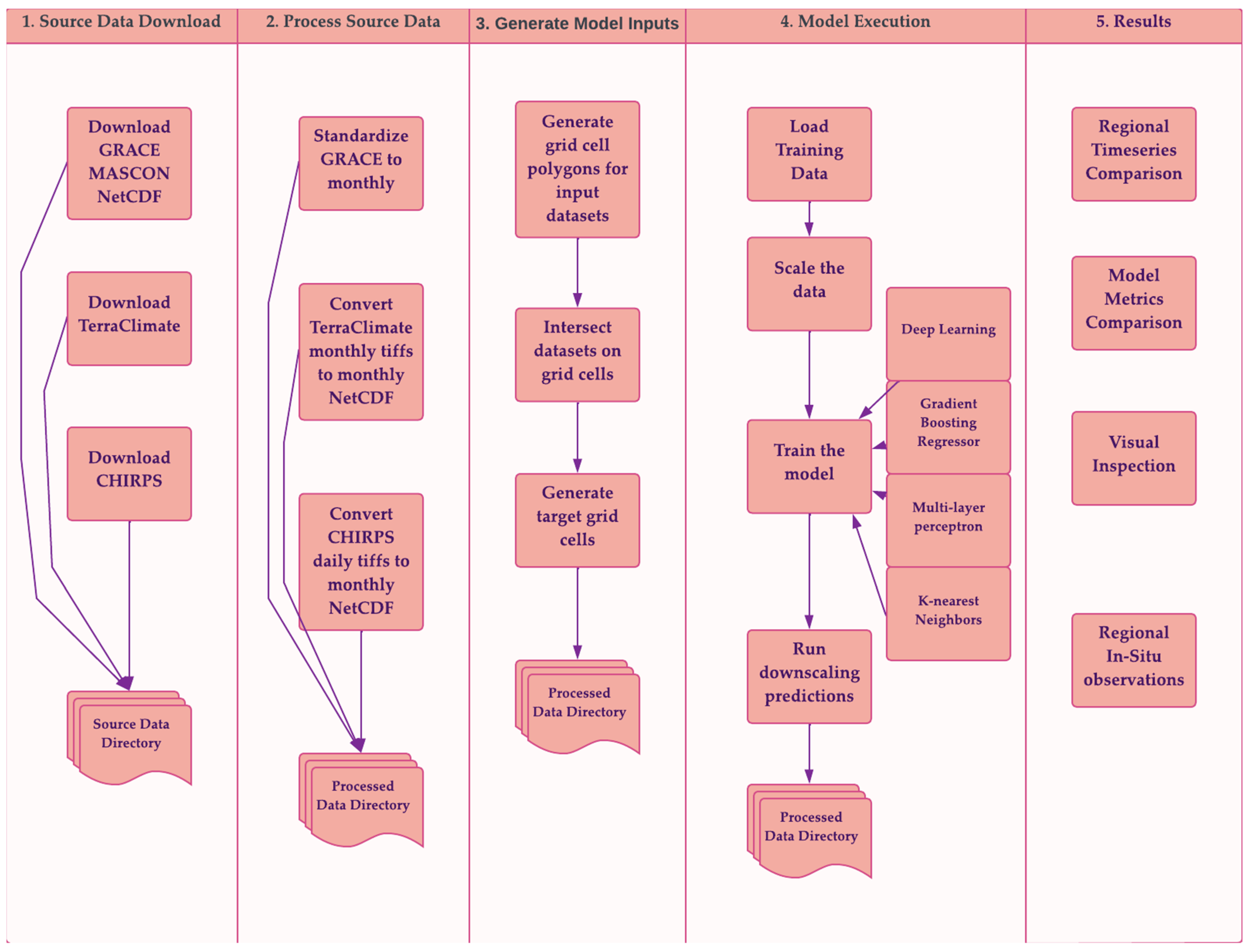
The objective of this effort is to develop an end-to-end workflow called the GRACE Downscaler (Figure 1), which facilitates the development, evaluation, and intercomparison of machine learning models used for downscaling GRACE data. This study provides a readily available source code for researchers to explore and effectively utilize GRACE data. The framework source code for this project is made available via GitHub, thus allowing re-searchers to replicate and reproduce the workflow for any region of interest. As a test case, we implement the workflow over the state of Mississippi in the United States.
The machine learning modeling framework is built on reliable and well-tested existing open-source packages. It provides a blueprint which users can modify and adapt for their own use case with ease.
2. Materials and Methods
2.1. Project Template
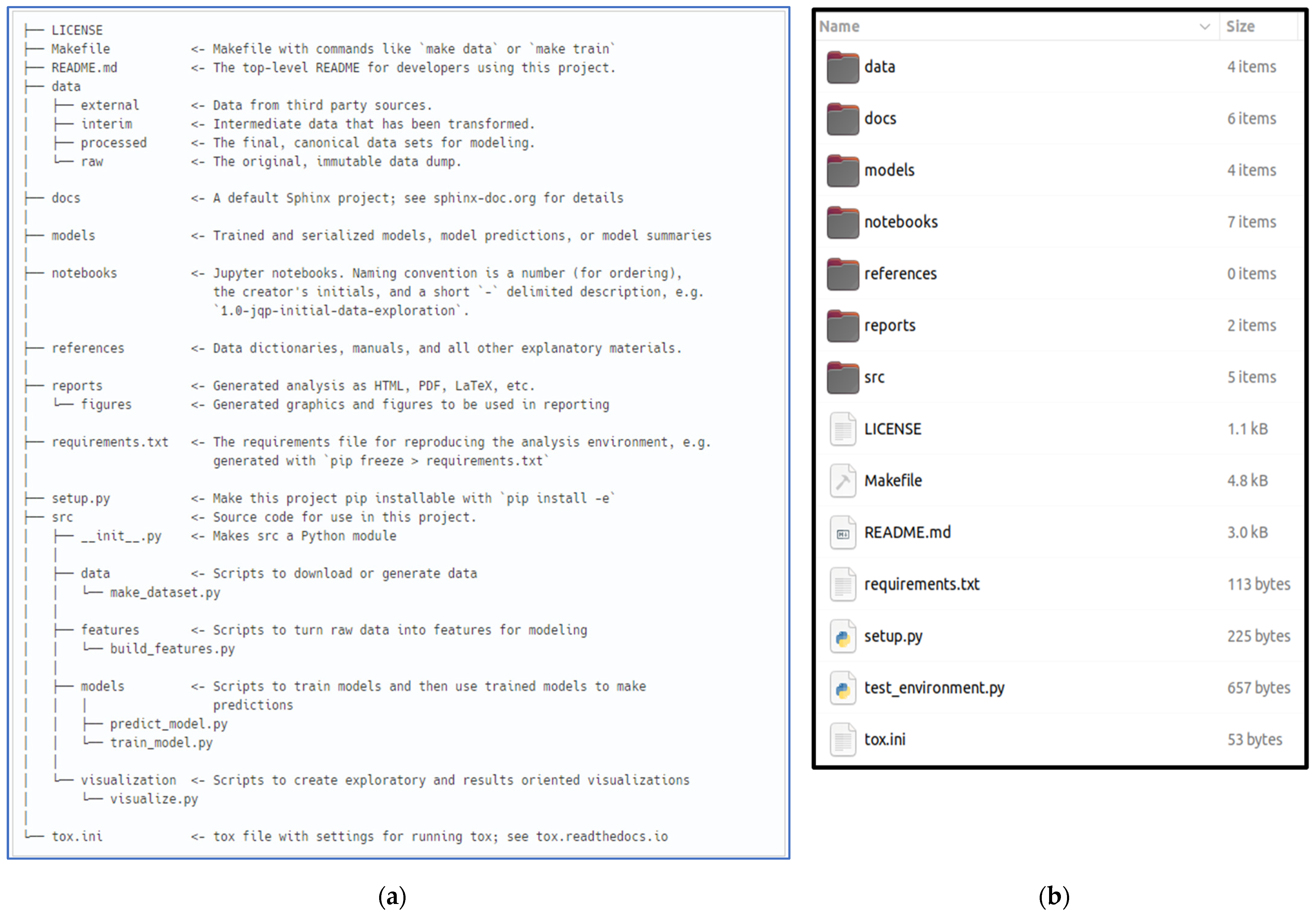
The Python project for GRACE Downscaler was generated using the Cookiecutter Data Science template [20]. This template provided an easy to use, flexible, and standardized project structure for organizing the project source code. The Cookiecutter Data Science template is executed using the command line utility tool of the Cookiecutter Python package [20]. Once executed, it initializes an empty project with a pre-built directory structure. Figure 2a is the representation of the project structure as generated by the Cookiecutter. Certain directories from the original template (Figure 2b) were deleted for clarity.
The Data Science Cookiecutter template is organized to make it easier for new users to quickly learn the contents of the source code. The lean directory structure reduces the learning curve for reproducing the analysis. It allows for smoother collaboration and version control. We recommend that researchers create a new project for each new region of interest. For instance, if a developer is creating multiple models across multiple regions, we recommend that each region of interest is spun off and initialized with its own standalone project directory. Since each region could potentially have different challenges, separating the source code will help with debugging and data management.
All the codes were developed through Jupyter Notebooks [21] for simplicity, ease of use, and shareability. Once the project is in a steady state, commonly used functions should be moved over into the source code directory. Since we were focused on rapidly developing as many models as possible, we did not spend any additional time in developing a model specific package. Additionally, since each model had slightly different parameters and workflows, we have not standardized functions. However, each notebook within the notebook’s directory was named clearly and numbered according to the order of execution so the location to modify can be more easily found.
2.2. Datasets
In recent GRACE downscaling publications, researchers have used a mix of categorical and numerical variables to train downscaling models [3,4,6]. These include variables that encompass land cover/land use change, digital elevation models, forcings from existing models such as Global Land Data Assimilation System (GLDAS), and other ancillary variables that influence the water balance, such as evapotranspiration, soil moisture, and snow water equivalent. This section highlights the datasets and variables that were used to help train the machine learning models for our study region. The justification for selecting each of the model input variables is presented.
All the variables that were selected contained enough data to generate monthly values for a significant portion across the GRACE time period. We have excluded variables such as land cover and land use change and digital elevation models as they typically do not change that drastically on a month-to-month basis. Having datasets that have variables with reasonable variations during the year is critical to develop a robust model that is sensitive to seasonality. There are several different theories on which methods are efficient for feature selection. Instead of spending significant amounts of time on iterating for the best model-specific feature, we left it up to the model to do the heavy lifting, regardless of the input features. Since we are interested in quickly iterating over multiple models, a rigorous feature selection process was avoided to maintain simplicity.
2.2.1. GRACE Data
The GRACE mascon data from the NASA Jet Propulsion Laboratory (JPL) is the target dataset for downscaling. The GRACE mascon data is recommended for hydrological and mass change application [22]. It is processed using de-striping algorithms to overcome the limitations of the raw GRACE data. The sensor has an infrequent temporal resolution of approximately one month, which limits its ability to capture short-term changes and variability in Earth’s gravimetric field. The stripping can be an artifact of the algorithms used to model not only the gravimetric field, but the atmospheric and oceanic tidal effects as well [16]. The geographic extent of the GRACE data spans −180 through 180 longitude and −90 through 90 latitude, and the spatial resolution is 0.5 degree. The temporal extent spans April 2004 to present. There is a two-month lag to the current date due to the processing schedule.
The GRACE mascon data product is made of mass concentration blocks (mascon). It is a form of gravity field basis function to which GRACE’s inter-satellite ranging observations are fit. Using a mascon simplifies the process for implementing geophysical constraints [22].
2.2.2. Climate Hazards Group Infrared Precipitation with Stations (CHIRPS)
CHIRPS is a quasi-global rainfall dataset spanning from 1981 to the present [23]. CHIRPS integrates 0.05-degree resolution satellite images with in situ rainfall station data to develop a gridded rainfall time series for trend analysis and seasonal drought monitoring. The geographic extent covers −50 through 50 degrees latitude and all longitudes. Due to the significance of precipitation in driving groundwater recharge, the high resolution of CHIRPS plays a critical role in developing the downscaling model.
2.2.3. TerraClimate
TerraClimate is a global dataset of monthly climate and climatic water balance for global terrestrial surfaces from 1958 to 2020 [24]. It has a monthly temporal resolution and a ~4 km (1/24 degree) spatial resolution. The dataset is available for the period from 1958 to 2020 and is updated annually. TerraClimate data has variables such as Actual evapotranspiration, Palmer Drought Severity Index, and soil moisture that influence groundwater recharge. Table 1 highlights the TerraClimate variables and the justification for their use in this study.
2.2.4. Rationale of Data Source Selection
The integration of CHIRPS and TerraClimate datasets with GRACE data provides complementary information for downscaling, as these datasets capture different aspects of the hydrological cycle. While CHIRPS focuses on precipitation, TerraClimate offers a broader range of variables, including temperature, evapotranspiration, and soil moisture. This complementary information can help to better capture the complex interactions between GRACE-derived terrestrial water storage and other hydrological components, thus improving the downscaled output [25]. Both CHIRPS and TerraClimate datasets have been extensively employed in various hydrological research applications, including drought monitoring [26,27], water resource management, and climate change impact assessments [28]. Their widespread use and ease of access has made them an ideal candidate for demonstrating the framework.
2.3. Data Processing
2.3.1. Download Source Data
The first notebook is set up to download the source data from their respective sources. The geemap Python package [29] is used in conjunction with other common Python packages to download the raw data. The package geemap is a wrapper around Google Earth Engine (GEE), a popular cloud-based geospatial data catalog and geoprocessing platform. Since GEE is free for research, non-commercial, and educational use, we have leveraged its highly efficient computing resources to download the TerraClimate data. The shapefile [30] identifying the region of interest (ROI) was converted to GeoJSON [31]. Geemap has a utility function to convert the GeoJSON file to a GEE-compatible format. Once converted, another utility function was used to download the clipped TerraClimate rasters to a directory within the raw data directory of the project.
The GRACE mascon data was downloaded from the Jet Propulsion Laboratory’s (JPL) OPEnDAP [32] data server. The siphon Python package [33] streamlined the process for iterating over the OPEnDAP directory contents. The latest GRACE Tellus and Scale Factors files were downloaded into a GRACE specific directory within the raw data directory.
Finally, the raw CHIRPS data was downloaded directly from the ClimateSERV web application [35]. Even though there was a Python package for accessing the different datasets available through the ClimateSERV application programming interface, it was more convenient to use the map interface. The ClimateSERV map interface has a tool to upload a region of interest and to download the compressed file of rasters for a selected date range. These data are uncompressed and saved to the raw data directory.
2.3.2. Process Source Data
The source data from the respective sources were converted into the NetCDF data format [36] for ease of use. The NetCDF format standardized the data and made it easier to manipulate and visualize through existing web/desktop-based applications. The xarray [37] and rasterio [38] Python packages were used in conjunction to generate a monthly mean of the CHIRPS, GRACE, and TerraClimate datasets.
Since GRACE data had missing months, it was necessary to normalize the date to generate machine learning model training input. The CHIRPS raw output comprised daily raster files that had to be aggregated to monthly intervals. The xarray resample function can automatically configure the appropriate time interval and generates the mean for the selected cadence. The source data is processed in the second notebook with the output saved inside the processed data directory.
2.3.3. Generate Model Inputs
The data quality of the model inputs is a significant driver of the model results [39]. For most applications of supervised machine learning models, the model output is only as good as the model input. Most machine learning models require the model inputs to be in tabular data format. The third notebook in the workflow houses the logic for generating the tabular model input. The output of this notebook is stored within the processed data directory. This step of the workflow is unique and the first of its kind for downscaling modeling.
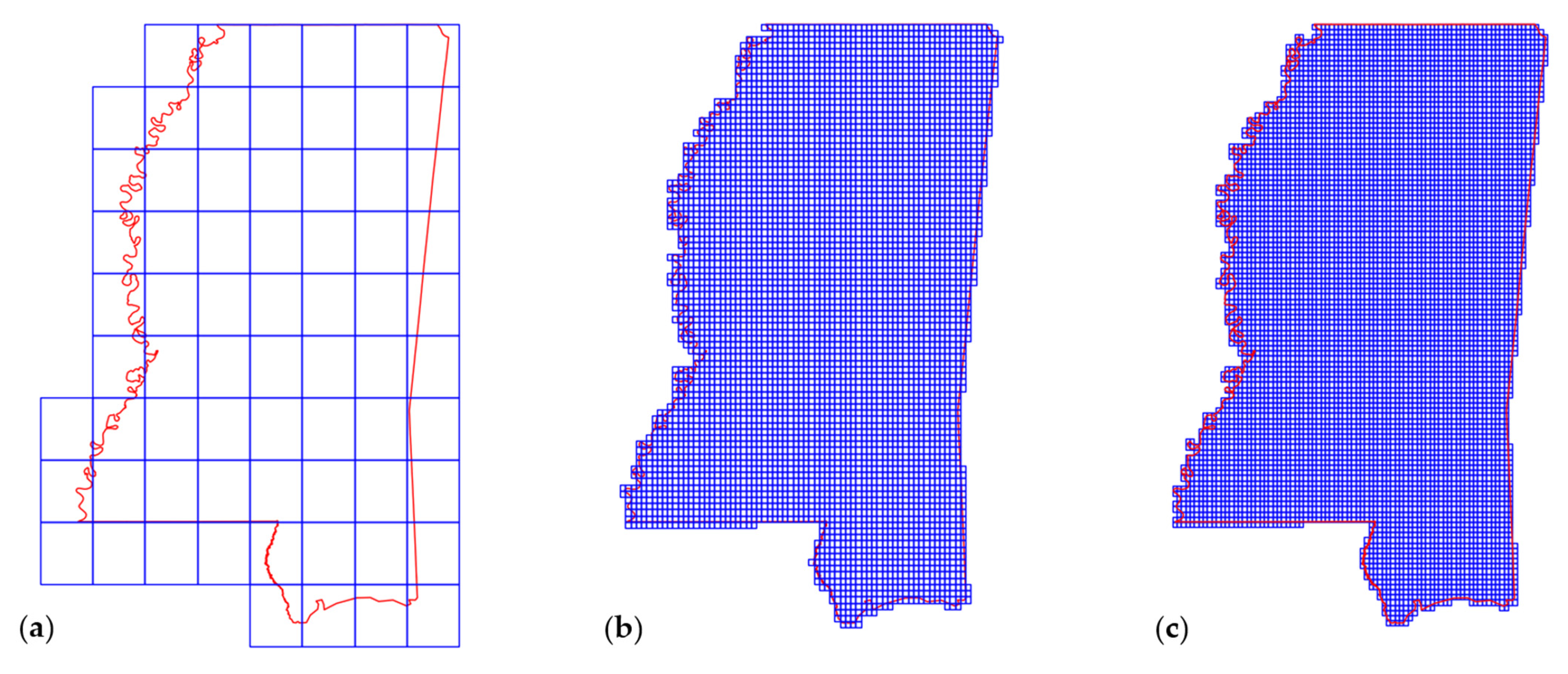
The vector-based grid cells for the three datasets were generated using the xagg Python package [40]. The package provided an easy-to-use interface to convert raster polygons from the NetCDF format into vector-based polygons. Xagg converts the data using area-weighted average from the relative overlap between the grid pixels and polygons. The output polygon size is influenced by its distance from another polygon. Xagg generates the grid polygons based on the bounding box extent of the input grid data. In other words, it generates more polygons than the actual shape of the input region. Thus, an additional intersection is applied on the xagg polygons to obtain a clean representation of the final grid cell polygons. Figure 3 is a sample output of the grid cell polygons for the three input datasets generated using xagg.
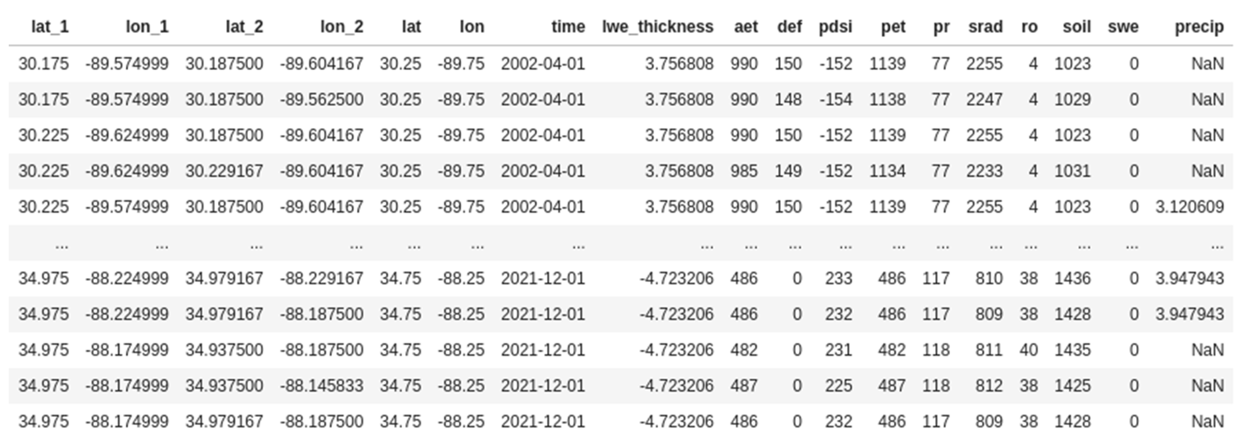
The generated vector-based polygons are accessible via the GeoPandas Python package [41]. The conversion of the grid cells to GeoPandas dataframes enabled the intersecting of the varying grid cell resolutions into a single row-based dataset. This provided unique values for all the intersecting grid cells based on the highest grid resolution. For instance, the vector-based intersection of the grid cell resolution of GRACE at 0.5 degree, CHIRPS at 5 km, and TerraClimate at 4 km will generate a final unique grid cell at or below 4 km. Figure 4 is the tabular representation of the final processed data.
The lat_1 and lon_1 columns are the grid cells corresponding to the CHIRPS dataset, the lat_2 and lon_2 columns are the grid cells corresponding to the TerraClimate dataset, and the lat and lon columns are the GRACE grid cells. The first six lines highlight the unique values of the CHIRPS values, while the other grid cell values remain constant. The lwe_thickness is the GRACE dataset value; this is the output variable for the training da-taset. The aet, def, pdsi, pet, pr, srad, ro, soil, and swe are from the TerraClimate dataset and are a significant portion of the input features for the model training dataset. Finally, the precip column, which is another input feature for the model training dataset, is derived from the CHIRPS dataset. The TerraClimate dataset has the highest resolution and drives most of the variability for generating the downscaling model.
The target grid for downscaling was generated in this notebook using the xagg package as well. First, a rectangular grid was created from the bounds of the region extents. Using the numpy arrange function, the grid cell latitude and longitude values are generated for a selected resolution. We generated a target grid with 1 km resolution. A sample NetCDF dataset is created from the target latitude and longitude values. This dataset is then run through xagg for generating vector-based grid cell polygons. They are then intersected against the shapefile of interest to only select the grid cells that fall within the region. The final target grid polygons are then intersected with the CHIRPS and TerraClimate dataset. In the target grid, the GRACE latitude and longitude values are replaced by the target grid cell latitude and longitude values.
The resolution of the target grid is typically a lot more data- and computationally intense than the existing datasets. Most regular machines will not be able to handle the intersection of the target grid cells and the datasets of interest. To overcome this challenge, we looped over each GRACE timestep and replaced the GRACE timestep with the target grid cells values. The output intersection for each timestep was saved out to a parquet file [42]. This significantly reduced the required storage and computational needs. For instance, originally, the target grid csv file was approximately 100 MB for a single timestep. However, converting the final intersection into a parquet file, the target values for a timestep required only 500 kB.
2.4. Models
The framework is designed such that users can implement any machine learning model of interest. Four models were developed for the study region. A deep learning model was developed using the Keras [43] Python machine learning package. Keras is a deep learning Python API written on top of the popular TensorFlow machine learning package. It is a simple, flexible, and powerful tool for developing a wide array of machine learning models. It is the most popular framework for developing deep learning models. The remaining three regression-based machine learning models were built using the scikit-learn [44] Python machine learning package. Scikit-learn has many classification, regression, and clustering algorithms such as support-vector machines, random forests, gradient boosting, and k-means, and is designed to interoperate with existing Python numerical and scientific libraries, such as numpy and scipy. It is one of the most popular machine learning packages in the data science community.
The four models for the study were chosen due to their popularity, simplicity, and ease of implementation. A multi-layer perceptron was implemented successfully for downscaling rainfall over an arid region [45]. For the k-nearest neighbors model, this was a novel approach and was considered as an experimental choice, while the gradient boosted decision tree and deep learning are widely used models.
For each model workflow, the training input was divided into an 80–20% split for training and testing. The scikit-learn standard scaler was applied to standardize the data. This helped in adjusting for outliers and preventing the model from computation errors due to large or undefined values. The model outputs were then run through a series of statistical functions to evaluate their effectiveness.
2.4.1. Deep Learning Model
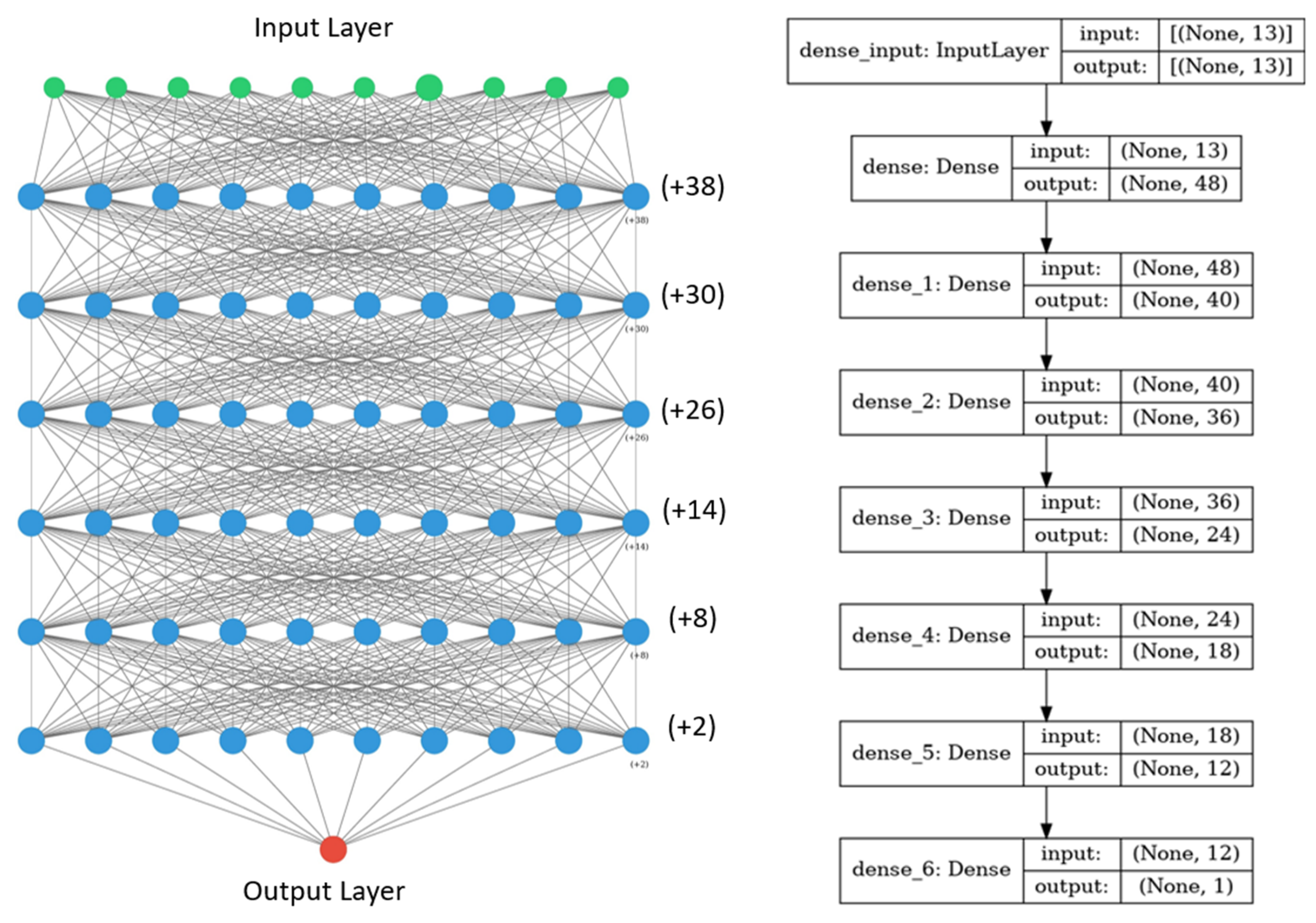
The deep learning (DL) model for the study region was built using the Keras Sequential model [43]. The Sequential model consists of a stack of neural network layers strung together to form a robust neural network. The number of layers and other hyperparameters were determined through an iterative trial and error process. Figure 5 is the graphical and tabular representation of the finalized model for the Mississippi problem. In this exercise, we used GRACE and other publicly available data to train an ML model to predict groundwater levels.
The finalized model consists of six layers, with 5687 trainable parameters. The layers and their relevant parameters were tweaked until the learning rate and loss parameters for the model were decreasing at a reasonable rate. We were able to build a sophisticated deep learning model from minimal effort. The number of hidden nodes within each layer is insignificant after a certain threshold. That threshold for the number of layers and the hidden nodes within each layer are hard to determine and require a significant amount of testing and iterations.
2.4.2. Gradient Boosting Regressor Model
A gradient tree boosting or gradient boosted decision tree (GBDT) is a generalization of boosting to arbitrary differentiable loss functions [46]. GBDT is an accurate and well-established procedure that is used for both regression and classification problems across a variety of domains. It is an additive model, meaning that several weaker models are trained against the training set and are brought together to form a single composite model.
The GBDT was executed with the following parameters: number of estimators = 300, max tree depth = 100, minimum samples split = 23,632 (default), learning rate = 0.01, and loss function set to the squared error. The greater the number of estimators, the more boosting stages. GBDT is robust to over-fitting, thus many estimators were selected to help with the accuracy. The maximum tree depth and learning rate were chosen after some trial and error. The minimum samples split was selected based on the number of observations per timestep. Finally, the squared error loss function was selected since it was the default recommended for regression due to its superior computational properties.
2.4.3. Multi-Layer Perceptron Regressor Model
The multi-layer perceptron (MLP) is a supervised learning algorithm [44]; it can learn a non-linear function approximator for either classification or regression. It is different from logistic regression in that between the input and the output layer, there can be one or more non-linear layers, called hidden layers. This is one of the most used neural network machine learning models. It uses backpropagation with a few different activation functions to compute the final output.
The MLP model was run with the following parameters: hidden layer size = (24, 18, 12, 6, 4), batch size = 23,632, solver = limited-memory Broyden–Fletcher–Goldfarb–Shanno algorithm (LBFGS), activation function = rectified linear unit, and learning rate = 0.001. The hidden layer size was determined through trial and error. After a certain threshold, the local development environment crashed due to a lack of memory. It was designed to be close to the deep learning model, after a few iterations an increase in the hidden layer size was hurting model performance. The final configuration worked reasonably well. The batch size was selected based on the number of observations per timestep. The solver LBFGS is a well-validated solver, and was chosen as it is recommended for datasets with a smaller sample of training data. The activation function was the default value, as suggested by scikit-learn. The learning rate was selected arbitrarily and did not have any significant impact on the final output.
2.4.4. K-Nearest Neighbors Regressor Model
Neighbors-based regression is used in cases where the data labels are continuous. The label assigned to a query point is computed based on the mean of the labels of its nearest neighbors. The k-nearest neighbors (KNN) regressor implements learning based on the k-nearest neighbors of each query point, where k is an integer value specified by the user. The target is predicted by local interpolation of the targets associated of the nearest neighbors in the training set.
The KNN regressor model was run with the following parameters: number of neighbors = 20, weights = distance, and algorithm parameter = auto select. The number of neighbors was set to 20 through trial and error. The weights parameter was set to distance. The nearby neighbors were weighted by the inverse of their distance, meaning, closer neighbors of a query point will have a greater influence than neighbors which are further away. The auto algorithm detected the best nearest-neighbors algorithm based on the input values. The KNN model was one of the fastest models for execution.
3. Results
After the models were compiled, the predictions were generated for a 1 km grid. This section outlines the model-specific metrics and output results. Each model notebook within the code repository contains some code to help evaluate the model metrics and to visualize the model outputs.
The deep learning model took the longest to execute, whereas the KNN regressor model was the fastest. The simpler regression-based models KNN and gradient boosting performed better than expected. Even though they were much simpler, the model metrics were similar to the more complex deep learning model and neural network-based MLP model.
3.1. Model Metrics
The model metrics for the downscaling machine learning models are shown in Table 2. All the error metrics evaluated for the models are the standard metrics that are used to measure the effectiveness of the regression techniques. The R-squared is one of the better-known methods to quantify the correlation between the actual and predicted model values.
The KNN performed the best in terms of raw model metrics with an R-squared value of 0.996, while the MLP had the lowest performance, with an R-squared value of 0.836. The DL and GBR were nearly identical, with the GBR slightly outperforming the DL in mean absolute error. Even though these metrics provide a high-level overview of the model performance, they do not provide a full picture of the underlying results.
3.2. Model Validation
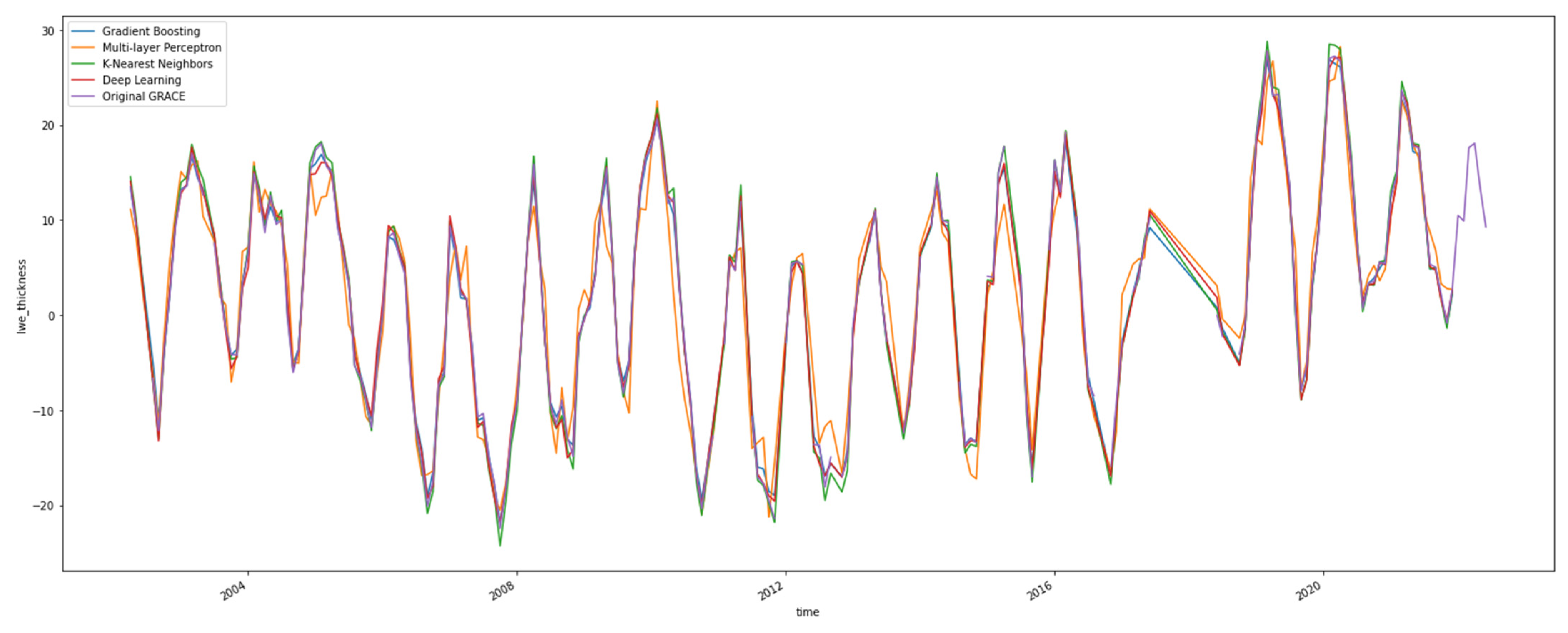
Validating the downscaled GRACE TWS dataset is challenging due to the lack of a comparable observed dataset. Thus, the next best validation methodology was to observe the variations in the timeseries generated at the regional level. This helps in evaluating the changes in conservation of mass at the regional level [7]. For each model, a timeseries value per timestep was generated by applying a mean across the grid cells. The timeseries chart for the models, along with the original GRACE data, is shown in Figure 6. For certain timesteps, the models underpredicted the original GRACE dataset, and for others they overpredicted the GRACE values. There are no discernable patterns on the model output results; however, all the models followed the general trend of the underlying GRACE dataset very well.
The regional timeseries for each of the models were compared against the original GRACE dataset with several metrics as shown in Table 3. The metrics were generated using the HydroErr Python package [47]. HydroErr has approximately seventy metrics to measure the hydrologic skill/fit of a model result. A few commonly used metrics, such as Nash–Sutcliffe efficiency [48], Spearman correlation coefficient [49], and Pearson correlation coefficient [50] were calculated to measure the model efficiency.
A mean value of the metrics was generated to obtain an overall metric of the model-generated timeseries values. The model timeseries metrics closely followed the model error metrics. The DL, GBR, and KNN all had a similar mean metric value. The MLP continued to underperform in comparison to the other three models. The DL and GBR regressor had slightly better timeseries metrics than the model error metrics.
3.3. Visual Inspection
Even though the model error metrics and time series metrics might indicate a statistically sound model, it is essential to check it visually to evaluate if the output is realistic. Within the code repository, there are a few code samples that users can replicate for visually inspecting the model output. The matplotlib package [51] was used to develop the timestep visualization. The xarray package leverages matplotlib under the hood to plot the NetCDF timestep values.
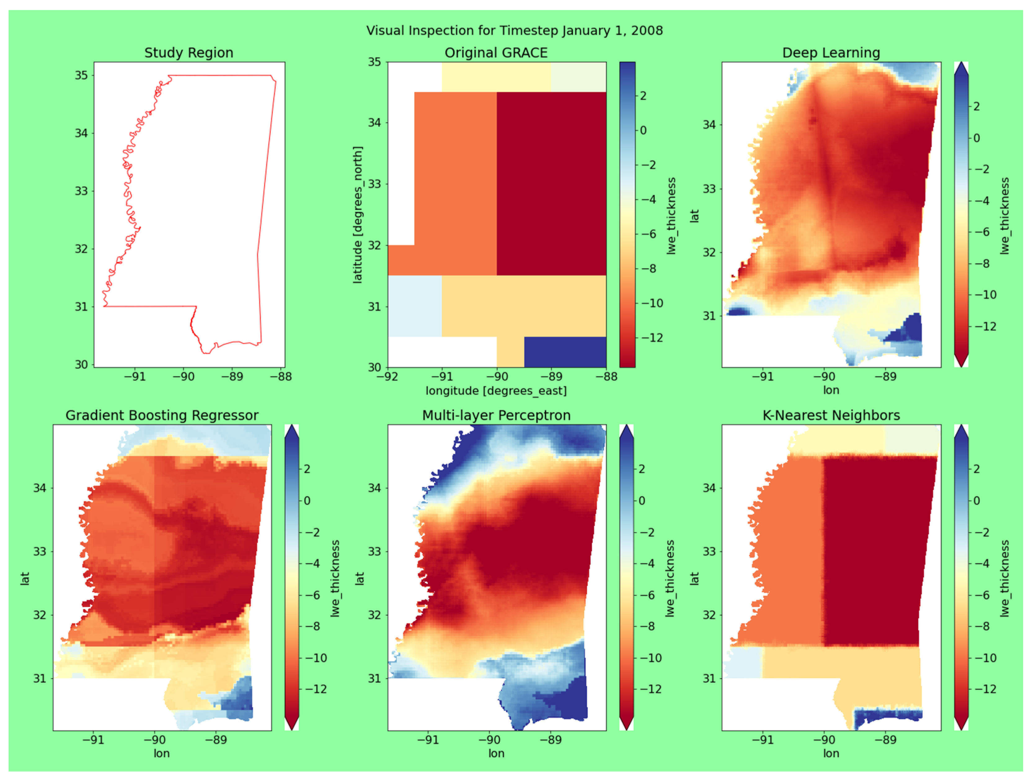
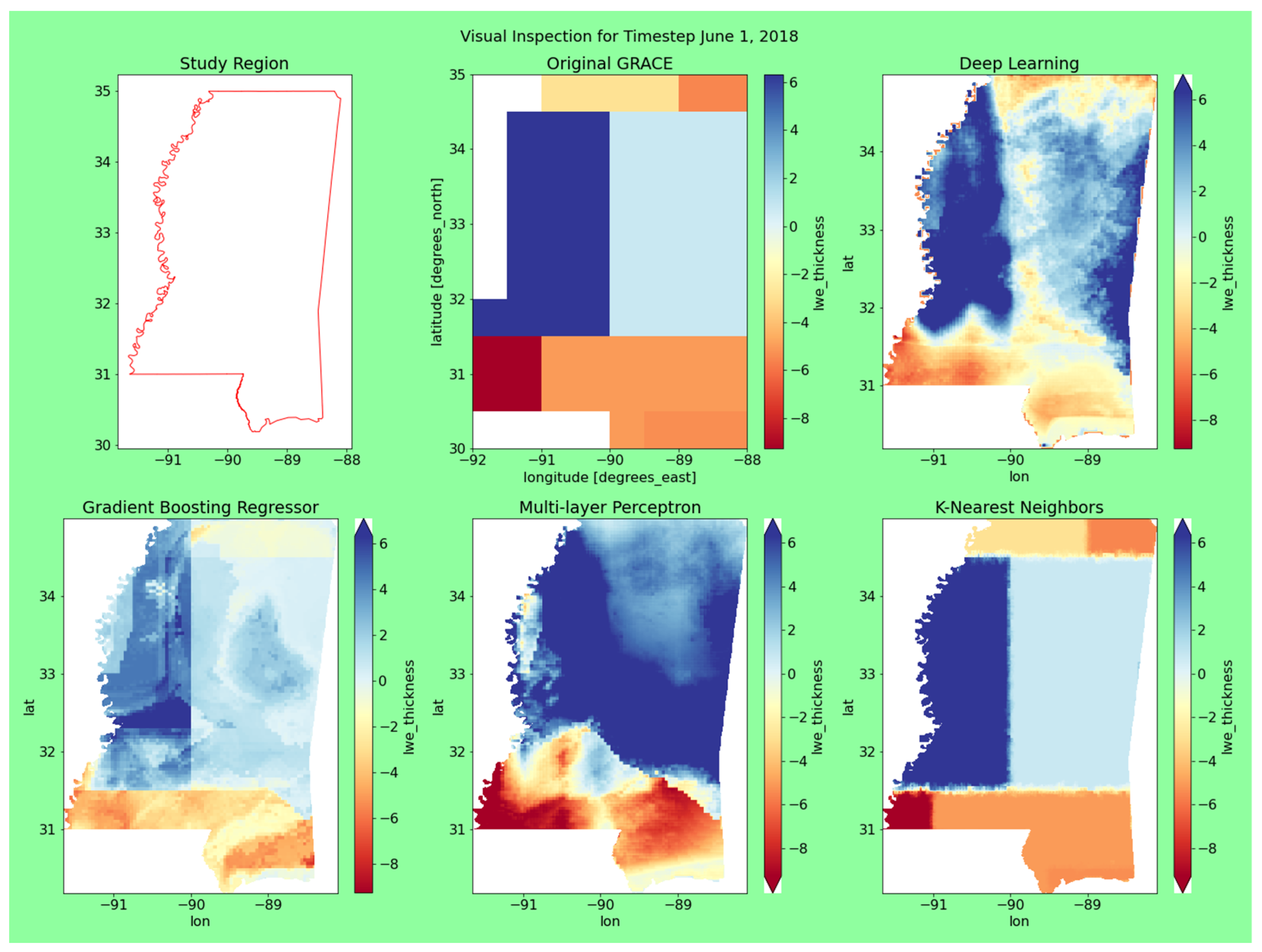
The model outputs for all the models, along with the original GRACE data at two different timesteps, are shown in Figure 7. The two timesteps for evaluation were January 2008 and June 2018; this was to ensure that we were inspecting time periods with rea-sonable variation and across seasons. The visual representation of each model varied significantly.
The DL model performed consistently. It was statistically sound and had a reasonably consistent spatial distribution. Even though the output values were greater, the overall trends matched up well with the original dataset. It was not as sensitive as GBR and not as uniform as the KNN. The DL model performed the best in terms of the final visual output.
The GBR was one of best performing models statistically; however, the outputs had a very inconsistent spatial distribution. The overall output values were close to the original dataset, but they seemed to be very sensitive to the input training variables. This highlights the need for conducting a visual inspection, as the outputs for the two time periods were not as consistent for use downstream.
The MLP produced a consistent spatial distribution, though the output values were consistently higher than the original dataset. For being the worst performing model from a statistical view, it performed reasonably well in visual evaluation.
The KNN outputs had very little variation across the timesteps. The results were akin to simply resampling the dataset. This highlighted the pitfalls of using a model outside its intended purpose. The model was not ideal for predicting a realistic downscaling result. It did not seem to take any of the input variables into account during training and had overfit the output results.
3.4. Case Study
Once the model development was at a mature stage, comparing it against regional water level data provided additional insights into the model accuracy. Generating a groundwater storage change curve from in situ well data and comparing it to the GRACE and downscaled storage changes was shown to be an effective method for gauging overall groundwater trend [52]. To further evaluate the trends for the study region, the well data for Sunflower County, Mississippi was extracted from the United States Geological Survey’s (USGS) groundwater web service. Sunflower County is within the Mississippi Delta region, it has significant agricultural activity and had a reasonable number of wells spanning the GRACE time period. Since the model was trained at the state scale, evaluating it at finer resolution, such as the county level, can help identify if the model results have reasonable variability.
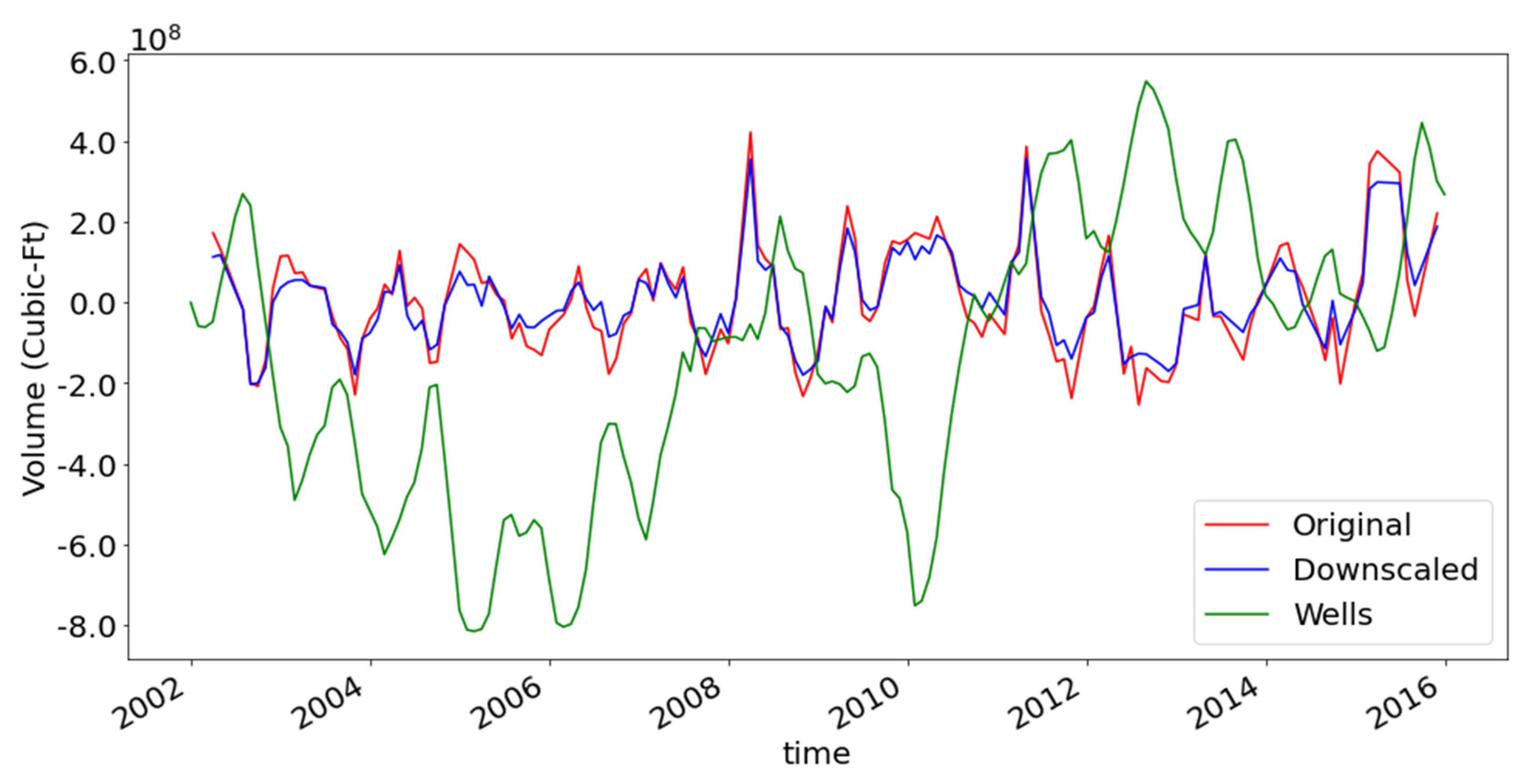
Using the methods implemented in the GRACE Groundwater Subsetting tool (GGST) and the Groundwater Data Mapper (GDM) [53,54,55], the groundwater storage volume timeseries was generated for Sunflower County, MS. The aquifer storage coefficient for generating the groundwater storage volume was derived empirically. The time period for analysis was from 2002 to 2016, to account for outliers. The derived storage volume, GRACE data, and DL downscaled storage volumes are shown in Figure 8.
The volume calculation in the GDM is sensitive to the aquifer storage coefficient, thus the volume timeseries at times significantly changes in comparison to the GRACE volume. However, some of the trends across years match well. For instance, the trends around 2009 and 2012 for the observed water level and GRACE are identical. Even though the peak volumes are not aligned in the time dimension, shifting the water level timeseries by a few weeks showed that the trends are better aligned. The trend rises and runs for the observed data in comparison to the GRACE data that show that the model has performed reasonably well for the overall time period. Further investigation with the aquifer storage coefficient value can help narrow the gaps between the observed and derived timeseries.
The discrepancies can also be attributed to in situ measurement errors, and hydrological model uncertainties. The in situ measurements were sparse and limited in this region of Mississippi. There was also significant pumping activity in the region due to agricultural activity. That, along with the aquifer characteristics, complicates the conversion from depth to water to water storage, thus adding to the uncertainty [56]. Moreover, since the process of deriving groundwater estimates relied exclusively on GLDAS, it was prone to its uncertainties, especially with critical variables such as evapotranspiration [57,58].
The downscaled volume trend follows the trend of the original GRACE data. This is an indication that the training data has reasonable variation. However, if there is lack of variability in the original versus downscaled timeseries, the variable selection process will need to be re-evaluated and represents a feedback loop in the proposed workflow.
4. Discussion
The proposed framework was created for the quick development and evaluation of machine learning models. With that stated, we urge users to be cautious with their final model selection. Each machine learning model is unique and has specific scenarios in which it performs well. The focus of this study was to demonstrate a high-level framework that can be replicated for any region of interest. We believe that even though a few of the methods we highlighted are common and have been typically used in general machine applications, this study helps to layout the general workflow for end users who are new to machine learning and downscaling methods. The model input generation workflow is a novel approach that streamlines the process for creating model training data. Regardless of the number of datasets and their varying resolutions, the approach we suggested simplifies the process and aids in generating a unique tabular input at the greatest grid cell resolution.
We have used two unique datasets for the training inputs, as there was a lack of high-resolution data for critical hydrological variables, such as soil moisture and evapotranspiration. Furthermore, there was a lack of such data that spanned across multiple years and regions. For an operational model, we recommend model developers use as many relevant and valid datasets they have access to in their study area. Once a model is developed, we recommend using the tools highlighted in the case study to perform validation against observed well data.
The workflow allows end users to prototype rapidly and measure the effectiveness of a model of interest. As of now, it does not have the functionality to automatically generate the downscaled results or to automatically generate the relevant error metrics. Our workflow is offered as a blueprint of methods that were assembled to allow for swift model creation and evaluation. The end users can leverage our code repository, but they need to make appropriate adjustments for their use case.
The approach presented in this work will help end users quickly iterate and develop multiple machine learning models with ease.
5. Conclusions
We present a comprehensive framework to create quickly and evaluate machine learning models for downscaling GRACE. Four machine learning models were developed—deep learning, multi-layer perceptron, k-nearest neighbors, and gradient boosting regressor. The deep learning and multi-layer perceptron performed well in capturing both the spatial and temporal intricacies of the input datasets. The gradient boosting regressor excelled at temporal statistics but fell short in capturing the spatial variability. The k-nearest neighbors model was misleading in terms of both spatial and temporal application and we recommend against using it for downscaling applications.
Current limitations of this framework include a lack of techniques or methods to address limitations of GRACE such as leakage factor [59,60,61], ability to validate in data sparse regions, and advanced bias correction. Future direction of the framework can include developing a method for assembling an ensemble model. Combining the strengths of multiple machine learning techniques, as well as integrating physics-based models with data-driven approaches, can lead to more accurate and robust downscaled GRACE data. Ensemble and hybrid approaches can help mitigate the limitations of individual models and better capture the complexity of the underlying hydrological processes.
We strongly recommend the implementation of such a downscaling framework only in instances where high-quality regional data are readily available. This approach ensures that the resulting high-resolution terrestrial water storage estimates accurately reflect the underlying hydrological processes and minimizes the biases or uncertainties stemming from the reliance on auxiliary datasets of suboptimal quality.
Author Contributions
Conceptualization, H.Y. and S.T.P.; methodology, S.T.P.; software, S.T.P.; validation, S.T.P. and L.D.Y.; formal analysis, S.T.P.; data curation, S.T.P.; writing—original draft preparation, S.T.P.; writing—review and editing, H.Y. and L.D.Y.; project administration, H.Y. and L.D.Y.; funding acquisition, H.Y. All authors have read and agreed to the published version of the manuscript.
Funding
This work was funded by a research grant awarded by the National Science Foundation (Award no: OIA 2019561).
Institutional Review Board Statement
Not applicable.
Informed Consent Statement
Not applicable.
Data Availability Statement
Code can be found a GitHub page https://github.com/IGWM/grace_downscaler (16 April 2023). All data used for this study are public domain and provided by the respective agencies’ data portals.
Acknowledgments
We appreciate the constructive feedback and insights provided by our colleagues and reviewers during the peer-review process which helped to strengthen the quality and impact of our work. We especially thank Greg Easson of The University of Mississippi, School of Engineering, Prabhakar Clement and Mukesh Kumar of The University of Alabama, as well as Norm Jones and Gus Williams of Brigham Young University.
Conflicts of Interest
The authors declare no conflict of interest.
References
- Miro, M.E.; Famiglietti, J.S. Downscaling GRACE Remote Sensing Datasets to High-Resolution Groundwater Storage Change Maps of California’s Central Valley. Remote Sens. 2018, 10, 143. [Google Scholar] [CrossRef]
- Pascal, C.; Ferrant, S.; Selles, A.; Maréchal, J.-C.; Paswan, A.; Merlin, O. Evaluating Downscaling Methods of GRACE (Gravity Recovery and Climate Experiment) Data: A Case Study over a Fractured Crystalline Aquifer in Southern India. Hydrol. Earth Syst. Sci. 2022, 26, 4169–4186. [Google Scholar] [CrossRef]
- Milewski, A.M.; Thomas, M.B.; Seyoum, W.M.; Rasmussen, T.C. Spatial Downscaling of GRACE TWSA Data to Identify Spatiotemporal Groundwater Level Trends in the Upper Floridan Aquifer, Georgia, USA. Remote Sens. 2019, 11, 2756. [Google Scholar] [CrossRef]
- Seyoum, W.M.; Kwon, D.; Milewski, A.M. Downscaling GRACE TWSA Data into High-Resolution Groundwater Level Anomaly Using Machine Learning-Based Models in a Glacial Aquifer System. Remote Sens. 2019, 11, 824. [Google Scholar] [CrossRef]
- Zhang, J.; Liu, K.; Wang, M. Downscaling Groundwater Storage Data in China to a 1-Km Resolution Using Machine Learning Methods. Remote Sens. 2021, 13, 523. [Google Scholar] [CrossRef]
- Yin, W.; Zhang, G.; Liu, F.; Zhang, D.; Zhang, X.; Chen, S. Improving the Spatial Resolution of GRACE-Based Groundwater Storage Estimates Using a Machine Learning Algorithm and Hydrological Model. Hydrogeol. J. 2022, 30, 947–963. [Google Scholar] [CrossRef]
- Vishwakarma, B.D.; Zhang, J.; Sneeuw, N. Downscaling GRACE Total Water Storage Change Using Partial Least Squares Regression. Sci. Data 2021, 8, 95. [Google Scholar] [CrossRef]
- Ali, S.; Khorrami, B.; Jehanzaib, M.; Tariq, A.; Ajmal, M.; Arshad, A.; Shafeeque, M.; Dilawar, A.; Basit, I.; Zhang, L.; et al. Spatial Downscaling of GRACE Data Based on XGBoost Model for Improved Understanding of Hydrological Droughts in the Indus Basin Irrigation System (IBIS). Remote Sens. 2023, 15, 873. [Google Scholar] [CrossRef]
- Chen, L.; He, Q.; Liu, K.; Li, J.; Jing, C. Downscaling of GRACE-Derived Groundwater Storage Based on the Random Forest Model. Remote Sens. 2019, 11, 2979. [Google Scholar] [CrossRef]
- Foroumandi, E.; Nourani, V.; Jeanne Huang, J.; Moradkhani, H. Drought Monitoring by Downscaling GRACE-Derived Terrestrial Water Storage Anomalies: A Deep Learning Approach. J. Hydrol. 2023, 616, 128838. [Google Scholar] [CrossRef]
- Gorugantula, S.S.; Kambhammettu, B.P. Sequential Downscaling of GRACE Products to Map Groundwater Level Changes in Krishna River Basin. Hydrol. Sci. J. 2022, 67, 1846–1859. [Google Scholar] [CrossRef]
- Zhang, G.; Zheng, W.; Yin, W.; Lei, W. Improving the Resolution and Accuracy of Groundwater Level Anomalies Using the Machine Learning-Based Fusion Model in the North China Plain. Sensors 2020, 21, 46. [Google Scholar] [CrossRef]
- Arshad, A.; Mirchi, A.; Samimi, M.; Ahmad, B. Combining Downscaled-GRACE Data with SWAT to Improve the Estimation of Groundwater Storage and Depletion Variations in the Irrigated Indus Basin (IIB). Sci. Total Environ. 2022, 838, 156044. [Google Scholar] [CrossRef]
- Wang, H.; Zang, F.; Zhao, C.; Liu, C. A GWR Downscaling Method to Reconstruct High-Resolution Precipitation Dataset Based on GSMaP-Gauge Data: A Case Study in the Qilian Mountains, Northwest China. Sci. Total Environ. 2022, 810, 152066. [Google Scholar] [CrossRef]
- Agarwal, V.; Akyilmaz, O.; Shum, C.K.; Feng, W.; Yang, T.-Y.; Forootan, E.; Syed, T.H.; Haritashya, U.K.; Uz, M. Machine Learning Based Downscaling of GRACE-Estimated Groundwater in Central Valley, California. Sci. Total Environ. 2023, 865, 161138. [Google Scholar] [CrossRef]
- Scanlon, B.R.; Zhang, Z.; Save, H.; Wiese, D.N.; Landerer, F.W.; Long, D.; Longuevergne, L.; Chen, J. Global Evaluation of New GRACE Mascon Products for Hydrologic Applications. Water Resour. Res. 2016, 52, 9412–9429. [Google Scholar] [CrossRef]
- Gemitzi, A.; Koutsias, N.; Lakshmi, V. A Spatial Downscaling Methodology for GRACE Total Water Storage Anomalies Using GPM IMERG Precipitation Estimates. Remote Sens. 2021, 13, 5149. [Google Scholar] [CrossRef]
- Delman, A.; Landerer, F. Downscaling Satellite-Based Estimates of Ocean Bottom Pressure for Tracking Deep Ocean Mass Transport. Remote Sens. 2022, 14, 1764. [Google Scholar] [CrossRef]
- Seyoum, W. GRACE TWSA Downscale in R 2022. Available online: https://github.com/wondy30/GRACE-TWSA-downscaling-ml (accessed on 3 March 2022).
- Cookiecutter Data Science. Available online: https://github.com/drivendata/cookiecutter-data-science (accessed on 3 March 2022).
- Kluyver, T.; Ragan-Kelley, B.; Rez, F.; Granger, B.; Bussonnier, M.; Frederic, J.; Kelley, K.; Hamrick, J.; Grout, J.; Corlay, S.; et al. Jupyter Notebooks—A publishing format for reproducible computational workflows. In Positioning and Power in Academic Publishing: Players, Agents and Agendas; IOS Press: Amsterdam, The Netherlands, 2016; pp. 87–90. [Google Scholar] [CrossRef]
- Wiese, D.N.; Yuan, D.-N.; Boening, C.; Landerer, F.W.; Watkins, M.M. JPL GRACE Mascon Ocean, Ice, and Hydrology Equivalent Water Height Release 06 Coastal Resolution Improvement (CRI) Filtered Version 1.0. Available online: https://podaac.jpl.nasa.gov/dataset/TELLUS_GRACE_MASCON_CRI_GRID_RL06_V1 (accessed on 25 September 2022).
- Funk, C.; Peterson, P.; Landsfeld, M.; Pedreros, D.; Verdin, J.; Shukla, S.; Husak, G.; Rowland, J.; Harrison, L.; Hoell, A.; et al. The Climate Hazards Infrared Precipitation with Stations—A New Environmental Record for Monitoring Extremes. Sci. Data 2015, 2, 150066. [Google Scholar] [CrossRef]
- Abatzoglou, J.T.; Dobrowski, S.Z.; Parks, S.A.; Hegewisch, K.C. TerraClimate, a High-Resolution Global Dataset of Monthly Climate and Climatic Water Balance from 1958–2015. Sci. Data 2018, 5, 170191. [Google Scholar] [CrossRef]
- Scanlon, B.R.; Zhang, Z.; Reedy, R.C.; Pool, D.R.; Save, H.; Long, D.; Chen, J.; Wolock, D.M.; Conway, B.D.; Winester, D. Hydrologic Implications of GRACE Satellite Data in the Colorado River Basin. Water Resour. Res. 2015, 51, 9891–9903. [Google Scholar] [CrossRef]
- Zhao, X.; Xia, H.; Pan, L.; Song, H.; Niu, W.; Wang, R.; Li, R.; Bian, X.; Guo, Y.; Qin, Y. Drought Monitoring over Yellow River Basin from 2003–2019 Using Reconstructed MODIS Land Surface Temperature in Google Earth Engine. Remote Sens. 2021, 13, 3748. [Google Scholar] [CrossRef]
- Wang, J.; Liu, G.; Zhu, C. Evaluating Precipitation Products for Hydrologic Modeling over a Large River Basin in the Midwestern USA. Hydrol. Sci. J. 2020, 65, 1221–1238. [Google Scholar] [CrossRef]
- de Andrade, J.M.; Ribeiro Neto, A.; Bezerra, U.A.; Moraes, A.C.C.; Montenegro, S.M.G.L. A Comprehensive Assessment of Precipitation Products: Temporal and Spatial Analyses over Terrestrial Biomes in Northeastern Brazil. Remote Sens. Appl. Soc. Environ. 2022, 28, 100842. [Google Scholar] [CrossRef]
- Wu, Q. Geemap: A Python Package for Interactive Mapping with Google Earth Engine. J. Open Source Softw. 2020, 5, 2305. [Google Scholar] [CrossRef]
- ESRI. ESRI Shapefile Technical Description; White Paper J-7855; ESRI: Redlands, CA, USA, 1998; p. 28. [Google Scholar]
- Butler, H.; Daly, M.; Doyle, A.; Gillies, S.; Schaub, T.; Hagen, S. The GeoJSON Format; Internet Engineering Task Force: Berlin, Germany, 2016; Available online: http://www.rfc-editor.org/info/rfc7946 (accessed on 7 September 2022).
- OPeNDAP. Available online: https://www.opendap.org/ (accessed on 7 September 2022).
- May, R.; Arms, S.; Leeman, J.; Chastang, J. Siphon: A Collection of Python Utilities for Accessing Remote Atmospheric and Oceanic Datasets 2022. Available online: https://unidata.github.io/siphon/latest/ (accessed on 11 March 2023).
- University of Idaho TerraClimate: Monthly Climate and Climatic Water Balance for Global Terrestrial Surfaces, Earth Engine Data Catalog. Available online: https://developers.google.com/earth-engine/datasets/catalog/IDAHO_EPSCOR_TERRACLIMATE (accessed on 10 October 2022).
- ClimateSERV. Available online: https://climateserv.servirglobal.net/ (accessed on 7 September 2022).
- UNIDATA NetCDF. Available online: https://www.unidata.ucar.edu/software/netcdf/ (accessed on 7 September 2022).
- Hoyer, S.; Joseph, H. Xarray: N-D Labeled Arrays and Datasets in Python. J. Open Res. Softw. 2017, 5, 10. [Google Scholar] [CrossRef]
- Rasterio Software 2022. Available online: https://github.com/rasterio/rasterio (accessed on 11 March 2023).
- Gudivada, V.; Apon, A.; Ding, J. Data Quality Considerations for Big Data and Machine Learning: Going Beyond Data Cleaning and Transformations. Int. J. Adv. Softw. 2017, 10, 1–20. [Google Scholar]
- Schwarzwald, K. Xagg 2022. Available online: https://xagg.readthedocs.io/en/latest/index.html (accessed on 11 March 2023).
- Levi, O.; Richards, M.; Fleischmann, M. GeoPandas. 2022. Available online: https://github.com/geopandas/geopandas (accessed on 7 September 2022).
- Apache Parquet Apache Parquet. Available online: https://parquet.apache.org/ (accessed on 12 September 2022).
- Bursztein, E.; Chollet, F.; Rasskin, G.; Jin, H.; Watson, M.; Zhu, Q.S. Keras: Deep Learning for Humans 2022. Available online: https://github.com/keras-team/keras (accessed on 7 September 2022).
- Pedregosa, F.; Varoquaux, G.; Gramfort, A.; Michel, V.; Thirion, B.; Grisel, O.; Blondel, M.; Müller, A.; Nothman, J.; Louppe, G.; et al. Scikit-Learn: Machine Learning in Python. J. Mach. Learn. Res. 2012, 12, 2825–2830. [Google Scholar] [CrossRef]
- Ahmed, K.; Shahid, S.; Haroon, S.B.; Xiao-jun, W. Multilayer Perceptron Neural Network for Downscaling Rainfall in Arid Region: A Case Study of Baluchistan, Pakistan. J. Earth Syst. Sci. 2015, 124, 1325–1341. [Google Scholar] [CrossRef]
- Friedman, J.H. Stochastic Gradient Boosting. Comput. Stat. Data Anal. 2002, 38, 367–378. [Google Scholar] [CrossRef]
- Roberts, W.; Williams, G.P.; Jackson, E.; Nelson, E.J.; Ames, D.P. Hydrostats: A Python Package for Characterizing Errors between Observed and Predicted Time Series. Hydrology 2018, 5, 66. [Google Scholar] [CrossRef]
- Nash, J.E.; Sutcliffe, J.V. River Flow Forecasting through Conceptual Models Part I—A Discussion of Principles. J. Hydrol. 1970, 10, 282–290. [Google Scholar] [CrossRef]
- Spearman, C. The Proof and Measurement of Association between Two Things. Am. J. Psychol. 1987, 100, 441–471. [Google Scholar] [CrossRef]
- Benesty, J.; Chen, J.; Huang, Y.; Cohen, I. Pearson Correlation Coefficient. In Noise Reduction in Speech Processing; Cohen, I., Huang, Y., Chen, J., Benesty, J., Eds.; Springer Topics in Signal Processing; Springer: Berlin/Heidelberg, Germany, 2009; pp. 1–4. ISBN 978-3-642-00296-0. [Google Scholar]
- Hunter, J.D. Matplotlib: A 2D Graphics Environment. Comput. Sci. Eng. 2007, 9, 90–95. [Google Scholar] [CrossRef]
- Barbosa, S.A.; Pulla, S.T.; Williams, G.P.; Jones, N.L.; Mamane, B.; Sanchez, J.L. Evaluating Groundwater Storage Change and Recharge Using GRACE Data: A Case Study of Aquifers in Niger, West Africa. Remote Sens. 2022, 14, 1532. [Google Scholar] [CrossRef]
- McStraw, T.C.; Pulla, S.T.; Jones, N.L.; Williams, G.P.; David, C.H.; Nelson, J.E.; Ames, D.P. An Open-Source Web Application for Regional Analysis of GRACE Groundwater Data and Engaging Stakeholders in Groundwater Management. JAWRA J. Am. Water Resour. Assoc. 2022, 58, 1002–1016. [Google Scholar] [CrossRef]
- Evans, S.W.; Jones, N.L.; Williams, G.P.; Ames, D.P.; Nelson, E.J. Groundwater Level Mapping Tool: An Open Source Web Application for Assessing Groundwater Sustainability. Environ. Model. Softw. 2020, 131, 104782. [Google Scholar] [CrossRef]
- Evans, S.; Williams, G.P.; Jones, N.L.; Ames, D.P.; Nelson, E.J. Exploiting Earth Observation Data to Impute Groundwater Level Measurements with an Extreme Learning Machine. Remote Sens. 2020, 12, 2044. [Google Scholar] [CrossRef]
- Brookfield, A.E.; Hill, M.C.; Rodell, M.; Loomis, B.D.; Stotler, R.L.; Porter, M.E.; Bohling, G.C. In Situ and GRACE-Based Groundwater Observations: Similarities, Discrepancies, and Evaluation in the High Plains Aquifer in Kansas. Water Resour. Res. 2018, 54, 8034–8044. [Google Scholar] [CrossRef]
- Long, D.; Longuevergne, L.; Scanlon, B.R. Uncertainty in Evapotranspiration from Land Surface Modeling, Remote Sensing, and GRACE Satellites. Water Resour. Res. 2014, 50, 1131–1151. [Google Scholar] [CrossRef]
- Yeh, P.J.-F.; Swenson, S.C.; Famiglietti, J.S.; Rodell, M. Remote Sensing of Groundwater Storage Changes in Illinois Using the Gravity Recovery and Climate Experiment (GRACE). Water Resour. Res. 2006, 42, W12203. [Google Scholar] [CrossRef]
- Chen, J.L.; Wilson, C.R.; Li, J.; Zhang, Z. Reducing Leakage Error in GRACE-Observed Long-Term Ice Mass Change: A Case Study in West Antarctica. J. Geod. 2015, 89, 925–940. [Google Scholar] [CrossRef]
- Huang, Z.; Jiao, J.J.; Luo, X.; Pan, Y.; Zhang, C. Sensitivity Analysis of Leakage Correction of GRACE Data in Southwest China Using A-Priori Model Simulations: Inter-Comparison of Spherical Harmonics, Mass Concentration and In Situ Observations. Sensors 2019, 19, 3149. [Google Scholar] [CrossRef] [PubMed]
- Mu, D.; Yan, H.; Feng, W.; Peng, P. GRACE Leakage Error Correction with Regularization Technique: Case Studies in Greenland and Antarctica. Geophys. J. Int. 2017, 208, 1775–1786. [Google Scholar] [CrossRef]
Figure 1.
Workflow diagram of the downscaler methods.

Figure 2.
(a) Screenshot of the directory structure of the Data Science Cookiecutter Template [20]; (b) Data Science Cookiecutter Template as rendered in a local development environment.
Figure 2.
(a) Screenshot of the directory structure of the Data Science Cookiecutter Template [20]; (b) Data Science Cookiecutter Template as rendered in a local development environment.

Figure 3.
Final converted grid cell polygons laid onto a region shapefile: (a) GRACE grid cells dimensions and locations; (b) CHIRPS grid cells; (c) TerraClimate grid cells.
Figure 3.
Final converted grid cell polygons laid onto a region shapefile: (a) GRACE grid cells dimensions and locations; (b) CHIRPS grid cells; (c) TerraClimate grid cells.

Figure 4.
Tabular preview of the model input data captured as a screenshot.

Figure 5.
Keras Deep Learning Model for Downscaling GRACE data in the state of Mississippi.

Figure 6.
Regional timeseries for the original GRACE data and the downscaled machine learning models over Mississippi. All values of lwe_thickness are in cm.
Figure 6.
Regional timeseries for the original GRACE data and the downscaled machine learning models over Mississippi. All values of lwe_thickness are in cm.

Figure 7.
Visual representation of the original GRACE and the model outputs for January 2008 and June 2018. All values of lwe_thickness are in cm.
Figure 7.
Visual representation of the original GRACE and the model outputs for January 2008 and June 2018. All values of lwe_thickness are in cm.


Figure 8.
Approximated change in groundwater storage volume for Sunflower County, Mississippi.


Table 1.
TerraClimate attribute descriptions. Adapted from [34].
Table 1.
TerraClimate attribute descriptions. Adapted from [34].
| Attribute/Band | Units | Description | Justification |
|---|---|---|---|
| aet | mm | Actual evapotranspiration, derived using a one-dimensional soil water balance model | One of the leading indicators of drought; Affects the groundwater recharge |
| def | mm | Climate water deficit, derived using a one-dimensional soil water balance model | Hydrologic variable that influences the sur-face water storage |
| pdsi | - | Palmer Drought Severity Index | Indicator of long-term drought conditions; Helps capture groundwater depletion |
| pet | mm | Reference evapotranspiration (ASCE Penman-Montieth) | A hydrologic variable that influences groundwater and surface water storage |
| pr | mm | Precipitation accumulation | Hydrologic variable influencing the surface water storage and groundwater recharge |
| ro | mm | Runoff, derived using a one-dimensional soil water balance model | Hydrologic variable influencing all the TWS components |
| srad | W·m−2 | Downward surface shortwave radiation | Hydrologic variable influencing drought |
| soil | mm | Soil moisture, derived using a one-dimensional soil water balance model | Influences soil moisture component of TWS |
| swe | mm | Snow water equivalent, derived using a one-dimensional soil water balance model | Influences the snow water equivalent com-ponent of TWS |
Table 2.
Model error metrics breakdown.
| Model | R-Squared | Mean Absolute Error | Mean Squared Error | Root Mean Squared Error |
|---|---|---|---|---|
| Deep learning | 0.961 | 1.911 | 6.948 | 2.635 |
| Gradient boosting | 0.964 | 1.752 | 6.381 | 2.526 |
| Multi-layer perceptron | 0.836 | 4.209 | 29.455 | 5.427 |
| K-nearest neighbors | 0.996 | 0.158 | 0.599 | 0.774 |
Table 3.
Model timeseries metrics.
| Metric | Deep Learning | Gradient Boosting Regressor | Multi-Layer Perceptron | K-Nearest Neighbors |
|---|---|---|---|---|
| Pearson correlation coefficient | 0.997551 | 0.998527 | 0.969011 | 0.999333 |
| Nash–Sutcliffe efficiency | 0.995073 | 0.996227 | 0.938837 | 0.996128 |
| Modified Nash–Sutcliffe | 0.934946 | 0.943833 | 0.775171 | 0.939307 |
| Spearman correlation coefficient | 0.997703 | 0.998340 | 0.968447 | 0.999118 |
| R-squared | 0.995108 | 0.997056 | 0.938982 | 0.998667 |
| Mean | 0.984076 | 0.986797 | 0.918090 | 0.986511 |
Disclaimer/Publisher’s Note: The statements, opinions and data contained in all publications are solely those of the individual author(s) and contributor(s) and not of MDPI and/or the editor(s). MDPI and/or the editor(s) disclaim responsibility for any injury to people or property resulting from any ideas, methods, instructions or products referred to in the content. |
© 2023 by the authors. Licensee MDPI, Basel, Switzerland. This article is an open access article distributed under the terms and conditions of the Creative Commons Attribution (CC BY) license (https://creativecommons.org/licenses/by/4.0/).
Share and Cite
MDPI and ACS Style
Pulla, S.T.; Yasarer, H.; Yarbrough, L.D. GRACE Downscaler: A Framework to Develop and Evaluate Downscaling Models for GRACE. Remote Sens. 2023, 15, 2247. https://doi.org/10.3390/rs15092247
AMA Style
Pulla ST, Yasarer H, Yarbrough LD. GRACE Downscaler: A Framework to Develop and Evaluate Downscaling Models for GRACE. Remote Sensing. 2023; 15(9):2247. https://doi.org/10.3390/rs15092247
Chicago/Turabian StylePulla, Sarva T., Hakan Yasarer, and Lance D. Yarbrough. 2023. "GRACE Downscaler: A Framework to Develop and Evaluate Downscaling Models for GRACE" Remote Sensing 15, no. 9: 2247. https://doi.org/10.3390/rs15092247
Note that from the first issue of 2016, this journal uses article numbers instead of page numbers. See further details here.