Article

Machine Learning and Deep Learning for the Built Heritage Analysis: Laser Scanning and UAV-Based Surveying Applications on a Complex Spatial Grid Structure

1
Department of Civil and Industrial Engineering, ASTRO Laboratory, University of Pisa, L.go Lucio Lazzarino, 56122 Pisa, Italy
2
Department of Energy, Systems, Land and Construction Engineering, University of Pisa, 56122 Pisa, Italy
3
IBS Progetti Chianciano Terme, 53042 Siena, Italy
4
Department of History, Representation and Restoration of Architecture, Sapienza University of Rome, Via del Castro Laurenziano 7/a, 00161 Rome, Italy
*
Author to whom correspondence should be addressed.
Remote Sens. 2023, 15(8), 1961; https://doi.org/10.3390/rs15081961
Submission received: 16 February 2023 / Revised: 31 March 2023 / Accepted: 6 April 2023 / Published: 7 April 2023

Abstract

:
The reconstruction of 3D geometries starting from reality-based data is challenging and time-consuming due to the difficulties involved in modeling existing structures and the complex nature of built heritage. This paper presents a methodological approach for the automated segmentation and classification of surveying outputs to improve the interpretation and building information modeling from laser scanning and photogrammetric data. The research focused on the surveying of reticular, space grid structures of the late 19th–20th–21st centuries, as part of our architectural heritage, which might require monitoring maintenance activities, and relied on artificial intelligence (machine learning and deep learning) for: (i) the classification of 3D architectural components at multiple levels of detail and (ii) automated masking in standard photogrammetric processing. Focusing on the case study of the grid structure in steel named La Vela in Bologna, the work raises many critical issues in space grid structures in terms of data accuracy, geometric and spatial complexity, semantic classification, and component recognition.

Graphical Abstract

1. Introduction

Surveying acquisitions, data interpretation, and 3D modeling are crucial for ensuring facility management [1] and refined safety assessment [2], identifying potential collapse mechanisms [3], and planning appropriate preventive interventions [4] for reticular, space grid structures of the late 19th–20th–21st centuries (Figure 1). Upstream of deformation analysis and structural simulation, there is, to date, a need for:
  • The rationalization and speed up of prevention and maintenance operations as well as structural health monitoring based on the observation and processing of surveying data [5];
  • The creation of rapid prototyping techniques and the use of specific representation methods to support scholars and operators (architects, engineers, restorers, historians) in returning faithful models and information to the broader public of users and public administrations involved in the infrastructure management process [6].
However, only a few references can be found today regarding the survey and geometric modeling phases of recent spatial grid structures. Recent research [1,7,8] has proven several complexities of the 3D data acquisition phase for this kind of structure in terms of spatial distribution [9], accessibility, size [10], transparent double-sided coverage of components, variation in detail, color and material [11,12], the presence of shadow areas generated by nodes and uprights, and geometric similarities between elements [13].
Beyond the acquisition phase, many problems have been raised in terms of processing the survey data (e.g., automating the identification and mapping) within raw point clouds or meshes of the characteristics of buildings [14,15], structures [16,17], and infrastructure [3,18] such as the shape, size, and location. In this context, artificial intelligence (AI)-derived techniques might become effective tools to assist in the detection of collapse mechanisms [19] or anomalies in the data [20], the diagnosis of problems and failures [21,22], and maintenance and recovery activities.

Research Aim

The aim of this work was to define a more objective approach for the interpretation of space grid structures starting from surveying, prior to restoration and monitoring activities, that relies on AI-based techniques for the semi-automated classification of structural components and for the connection of raw information, in terms of:
  • The application of proper data acquisition techniques to ensure the required levels of precision and reliability even in comparison to consolidated works on older constructions;
  • The characterization of geometric and spatial complexity for identifying structural elements, joints, and deteriorated components that require intervention or replacement;
  • The 3D component reconstruction from the scan data in the BIM environment.
The approach, tested here with reference to the pilot case study of the steel reticular structure La Vela in Bologna, was articulated in two ways:
  • On one hand, considering laser scan data, a supervised ML method, the random forest (RF) algorithm, was applied to assist in the classification (by type and by size) of the 3D architectural elements making up the structure, with a multi-level and multi-scale classification approach;
  • On the other hand, for the UAV-based photogrammetric processing, a DL model was leveraged for automated masking of the input images to improve and expedite the construction of a 3D dense cloud.
The classified 3D photogrammetric and laser scanning data of the structure were integrated and considered for further reconstruction of each geometrical component in 3D solid elements through fitting algorithms that foster the scan-to-BIM reconstruction process. The results were evaluated from the level of detail and reliability point of view by comparing the surveyed data with the reconstructed and project data.

2. State-of-the-Art: Supervised ML and CNN-Based Classification Methods

The use of ML and DL algorithms in the 3D surveying of built heritage is a rapidly growing field. Recent research in the domains of cultural heritage [14,23] and land surveying [24] has demonstrated that AI algorithms can be applied to analyze and interpret data collected from sensors and can process large amounts of 3D information in a more automated manner as well as identify features, structural and architectural components [25,26], damage mechanisms [16], or materials [27] that manual methods might miss.
A supervised ML algorithm, the random forest (RF) [28], generally used for image-based classification, has recently been applied for the semantic segmentation of 3D data to assist in different applications such as monitoring [29] and restoration [23], and even to support the scan-to-BIM process. Since the first studies by Weinmann [30] and Hackel [31] on geometry features that can be extracted from the point cloud, RF has been applied to support activities such as degradation analysis [21], the detection of architectural components and urban-scale objects [32], and the recognition of specific features of painting or sculpture. Matrone et al. [33] proved that the RF outperformed state-of-the-art DL methods for the point cloud classification task, allowing for better results in reduced times. This ensemble learning algorithm takes a reduced portion of the 3D point cloud acquired by a laser scanner or photogrammetry as input. In this sample dataset, each point in the cloud is associated with a label (class of objects) plus a set of characteristics (features) that distinguish one class from another. The latter can be geometric features such as curvatures, covariance, or color features. Then, multiple decorrelated decision trees are combined to make predictions on the class or label of each point of the 3D point cloud, and the final predictions are made through a voting scheme. Concerning the state-of-the-art on the topic, Teruggi et al. [34] extended this ML classification method by proposing a multi-scale and multi-resolution approach, hierarchically classifying 3D data at different geometric resolutions to ease the learning process and optimize the classification results. The cited references always referred to either the case of land surveying or architectural ancient heritage. To the authors’ knowledge, research has yet to dwell on the application of traditional supervised ML for the point cloud segmentation of diagrids and complex grid structures. On the other hand, DL offers a more promising approach in image-based classification because DL techniques, as a subset of ML, rely on a large amount of pre-annotated data and require no human extraction of features to discriminate between classes. In these terms, DL for image-based 3D reconstruction methods might provide high-quality texture information valid for the investigation of the current state of structures (e.g., the location of rust, cracks in metal structures, or color-related information). Convolutional neural networks (CNNs) are a type of DL architecture commonly used for semantic segmentation tasks [35,36] that can be trained on large datasets of labeled images to predict the class of each pixel. ResNet [37] and U-Net [38] are the primarily used types of CNNs.
In the domain of complex grid structures, previous research by Knyaz et al. [12] on the complex wire structure of the Shukhov Tower proposed a DL-based technique for the automatic generation of image masks. Classification using deep CNNs such as U-Net [38] and HRNetV2 [39] was developed to boost many steps of the image-based reconstruction pipeline and to improve the accuracy of structure-from-motion (SfM) and multi-view stereo (MVS) processing. Initially, the U-Net algorithm was created and trained but the quality of the image segmentation had to be improved for correct point matching. The HRNetV2 segmentation results were much more correct, although the model could not distinguish between thread-like structures in the foreground and background of the images. A new model, called WireNet, was therefore developed to improve the segmentation of the front and back parts of the tower. A preliminary image selection was carried out to eliminate the blurred and low-quality images captured during the complex field acquisition. The presented CNN architectures provide a starting point for the proposal of a DL method for image segmentation and masking prior to photogrammetric processing to support image-based 3D reconstruction.

3. Materials

3.1. La Vela Spatial Grid Structure

The double-layered spatial grid roofing called ‘La Vela’ is part of the larger project of the area of the UNIPOL Tower and its connected buildings, located in the northeastern part of Bologna. The covering structure was built in 2012 using circular tubular profiles joined by spherical nodes at the intrados and rectangular tubular profiles connected by rigid joints at the extrados, with a hemispherical end provided with threaded holes to which the diagonal rods are connected (Figure 2). The roofing system covers an area of 3600 m2, with a span between the lateral supports of about 50 m. Each extrados mesh of the grid structure is approximately 4 × 4 m and was initially enclosed by ETFE (ethylene-tetrafluoroethylene copolymer) membrane pressure cushions connected directly to the roof’s extrados profiles. The pattern orientation of each ETFE pneumatic module was designed to filter out direct solar radiation while allowing natural light to pass through. Parametric modeling was deployed to explore the variability of the system thus obtained, minimizing the solar factor and otherwise maximizing indirect light transmission.
The frame elements between the ETFE cushions were sized to form a system of eave channels, which could convey stormwater to collection points. Open Project Office developed the architectural structure, while Prof. Massimo Majowiecki and his Technical Office were responsible for the architectural project; their work is documented in [40]. Later on, specific studies on the roof, carried out by an interdisciplinary team at the Delft University of Technology, focused on the use of renewable energy and the optimization of the performance-oriented parametric design of the cladding system to satisfy the thermal comfort of the area underneath La Vela, dedicated to stores, and to provide under-roof spaces with an adequate daylight factor [41].
In 2019, La Vela’s ETFE membrane cushions were almost destroyed after an extreme weather event of heavy hail. Following the event, a survey of the structure was requested in order to reconstruct the roof panels with different materials; the task was entrusted to Errealcubo Studio. The 3D survey of La Vela provided in this context defined the baseline data for this research, while the original project information (Figure 3) was used for the reliability validation of surveying and reconstruction. The surveying activity, previously documented in [42], is briefly summarized in Section 3.2.

3.2. 3D Surveying and Data Acquisition

The steel space structure presented several bottlenecks related to roof accessibility, intervisibility, and dimension for the survey campaign. The problem of top–down intervisibility is a specific connotation of open spatial reticular structures that define a non-clear distinction between intrados and extrados areas. The specific cover is up to 20 m from the ground, making direct surveying almost impossible to plan to meet the strict design deadlines. Additionally, the roof develops in space according to curved generators with variable radii. Therefore, optimizing the point of view and reducing the shadow effect given by the structural elements becomes unpredictable. Due to the complexity of dealing with the different lighting conditions, the use of photogrammetry solely to survey the intrados and extrados was ruled out a priori; in addition, the impossibility of placing targets on the structure ruled out this approach. As a result, an integrated survey approach based on 3D laser scanning, mini-UAV photogrammetry, and topographic survey was proposed to minimize all of these bottlenecks in acquiring the sides of both structures.

3.2.1. Topographic Framework

The first step was to define a general XYZ reference system to support the image and range-based data orientation. All GCPs were located on the ground due to the inaccessibility of the roof. The 3D reference system for the whole survey was defined by three vertices, materialized on the wooden floor of the main terrace below the structure, and acquired by a total station. Four fixed targets were placed in the scene (T1, T2, T3, T4), while 10 mobile aluminum targets were located ad hoc to orient the images for each RPAS flight in the same reference system. For each of the three stations (S1, S2, S3), fixed and mobile GCPs were surveyed (Figure 4).

3.2.2. Global Photogrammetric Survey

A photogrammetric survey of the entire structure was planned in order to provide a graphical representation of the structure’s extrados. The RPAS used was a DJI Mavic mini 2, equipped with a camera set up at 4 mm of focal length, f/2.8, ISO 100, and 1/1000 s of exposure time. We planned a flight distance of 50 m from the ground with a GSD of 1 cm. The sub-centimeter precision required for the survey campaign and the use of ultralight RPAS for safety reasons ruled out the RTK positioning system. The network vertices and the four fixed GPCs were used to orient the block of 35 images in Agisoft Metashape software, from which an ortho-image was extracted. For a detailed photogrammetric campaign, the survey area was divided into nine quadrants of 5 × 5 to 6 × 6 square meshes.

3.2.3. Detailed Photogrammetric Survey

In this survey, the camera parameters were the same, while the flight altitude did not exceed 6–7 m relative to the roof surface, obtaining a GSD of about 2 mm. Eight separate flights were planned to preserve a longitudinal and lateral coverage of about 80%, reducing the image processing step to a maximum of 250 images for each block (Figure 5). The roof shape and the altitude variation led to the acquisition of both nadiral and oblique images, guaranteeing complete coverage and high precision in the 3D survey of construction details. In total, 1184 digital images were oriented, with the coordinates of each node determined by collimating the point in at least three images. The presence of 10 oversized windows hid the nodes of the underlying mesh, obliging the surveying of window corners and the corresponding points located in the structure intrados. Concerning the edge meshes, in two borders of the structure, solar panels obscured the nodes in several images, limiting the number of usable ones. As many nodes were detected in multiple flights, it was possible to compare coordinates, validate the process, and discard the incorrect values. All coordinates were collected in a coordinate list, with the extraction of the six distances (four sides and two diagonals) that characterized each mesh. The four nodes did not belong to the same plane, so the diagonals were skewed.

3.2.4. Range-Based Survey

The instrument positions were carefully planned to reduce interference and stress the relationship between the working distance, the dimensions of the individual components, and the data accuracy, in accordance with good practice in range-based imaging. In addition, a preliminary test of the optical instrument behavior on the metal structure was planned to verify the noise that might have affected the data quality. The 3D laser scanner survey process started evaluating a uniform distribution of the scans for each quadrant: one high-resolution scan (3–10 m) to frame a primary alignment network and low-resolution scans (6–10 m) to provide second-level information. This approach made it possible to reduce the shadow areas. The Focus S70 (Faro) was used to acquire 29 range maps (Figure 6). The primary network was oriented with the GPCs, while the second network was aligned using ICP and bundle adjustment techniques. Every range map was cleaned by filtering the data over a working distance of 30 m as well as by manually eliminating spurious data due to tangential noise. The clouds were merged and subsampled to a resolution of 5 mm to regularize the point distribution and optimize the global point cloud management.

3.2.5. Data Integration and Validation

The integration between the image-based and range-based data was carried out using common GCPs (Figure 7). The point cloud obtained from the 3D laser scanning defines a gold standard model helpful for inspecting the photogrammetric output locally (node extraction) and globally (mesh comparison) by extracting information to support the data modeling process. Concerning the local analysis, the extraction of 20 diameters and barycenters of the cylindrical nodes from the range-based point cloud allowed for a first comparison with the photogrammetric data, revealing a standard deviation of 3 mm. In addition, the six main distances for each mesh extracted from the image-based and range-based data were compared, with an average between 1 mm and a standard deviation of 2 cm. From the global point of view, metric verification took place within the CloudCompare software, with a comparison of 3D range-based and image-based data in the space (Figure 8). The deviation map showed that most of the distribution of the overlapping values was below 2 cm. In addition, the photogrammetric cloud indicated a homogeneous behavior, highlighting the accuracy of the photogrammetric cloud and excluding errors in the construction of the 3D data. These analyses validated the data reliability and the integrated model.

4. Methods

Given the complexity of the object of study and the availability and multiplicity of different types of information and representations derived from surveying, the research was developed by pursuing in parallel (Figure 9), on one hand, the work on the laser scanned point cloud (i) and, on the other hand, the work on UAV-acquired images and the products of photogrammetric processing (ii).
For the first point, the processing of the laser scanner survey involved the application of supervised ML techniques, in particular, the RF algorithm, to classify architectural components at different levels of detail on the unstructured point cloud. For the second point, an automatic image masking procedure, based on the use of artificial neural networks, was studied to exclude unwanted objects from images and to improve the results of photogrammetric processing. A third phase (iii) involved the evaluation of the results obtained for the two parts: the data fusion, and the subsequent construction of BIM components from classified point clouds. This latest part was tested on some significant meshes of the structure. Finally, the reconstructed model was compared to the available project data.
The software MATLAB, with its Statistics and Machine Learning Toolbox and Deep Learning Toolbox, was considered to implement the AI algorithms presented. The methodology and related results in application to the La Vela structure are illustrated according to the subdivision into phases (i), (ii), and (iii), respectively.

4.1. Supervised Machine Learning for the Classification of Laser Scan Data

A multi-level and multi-resolution (ML-MR) classification approach was run for the range data processing (Figure 10). The La Vela structure was classified by creating a hierarchy of classes between the elements that compose the grid, based on increasingly more detailed characteristics: from the most general class (1st level), in which the elements are distinguished by architectural type, to the most specific one (3rd level), in which the elements are distinguished by their size. Different levels of resolution were identified to subdivide the structure concerning the level of detail of the single elements making up the space grid structure.
The classification method was derived from the successful tests by [43,44,45] on the application of the RF for the point cloud classification of heritage objects. The related studies regarding geometric feature importance are discussed by [30,31]. The ML-MR method, which relies on a hierarchical classification approach, follows the procedure proposed by [34] for the case of heritage objects.
The ML-MR workflow is articulated as follows:
  • The original point cloud is subsampled to provide different levels of geometric resolution;
  • Each time, at the various levels of detail, different component classes are identified on a reduced portion of the dataset (training set), and appropriate geometric features are extracted to describe the distribution of 3D points in the point cloud. Together, these data allow for the training of a RF algorithm to return a classification prediction (class of a 3D point) at the chosen level of resolution;
  • Classification results at the lowest level of detail are back-interpolated onto the point cloud at a higher resolution to restore a higher point density. The 3D points classified as belonging to a given class constitute the basis for another classification at the highest level of detail.
The process is iterative and continues until full resolution, at the most detailed semantic segmentation level, is achieved. At each iteration, the performance of the classifier is stressed in terms of accuracy, precision, recall, and F-measure. The choice of a ML-MR method is motivated by the following reasons:
  • Classifying the entire point cloud at maximum resolution in a single step is very complex. It leads to overloaded computational efforts and long training times related to a high number of geometric features and the size of the dataset.
  • An excessive number of semantic classes should subdivide the point cloud. This would lead to misclassification issues if classes of components share very similar features.

4.2. Deep Learning for Automated Masking of UAV Images Prior to Photogrammetric Processing

Regarding the photogrammetric processing part, eight blocks of images progressively processed by RPAS on each flight mission (see Section 3.2.3) were considered as the starting point. In total, 1184 digital images were used for the image-based reconstruction of La Vela’s extrados, divided into eight sections, each corresponding to a photogrammetric block.
Figure 11 shows the point clouds obtained from the raw processing related to each flight mission. The reconstruction of the background elements of the photo prevailed, as opposed to the components of the space grid structure, which were perceived as noise. This difficulty, related to the separation of foreground objects, leads to poor details for the point cloud of the structure and incredible details for the background (objects of the scene deemed unnecessary). The detection and identification of the areas of the image that enclose the structure could become a critical issue in structure from motion processing for other similar space grid constructions. In this situation, image masking techniques might enable the exclusion of certain areas of each image that contain background elements.
As such, the creation of the point cloud might be carried out by considering only the elements of the structure that are of interest. However, manual image masking has proven to be time-consuming. To overcome this problem, the DeepLab v3+ architecture [46], implemented on a pre-trained ResNet-18 network [37], was leveraged for the task of background–foreground separation, starting from a reduced set of manually annotated images (Figure 12). The minimum batch size of eight reduced memory usage during training, and the maximum number of epochs was set at 30. The procedure included:
  • Labeling. A set of ground-truth images was labeled by assigning a label to each pixel, with this operation being conducted manually on a chosen set of images. This manual masking process was performed via Agisoft Metashape software. The data were then extracted to constitute a specific folder of labeled images associated with the ground-truth images folder (Figure 13).
  • Data augmentation. To improve the neural network’s ability to generalize over a larger dataset, data augmentation techniques were envisioned during training. Such techniques involve transformation operations such as translation, rotation, and reflection to generate new augmented samples from the original ones. Data augmentation reduces overfitting by avoiding training on a limited set, preventing the network from storing specific characteristics of the samples.
  • Image adjustment strategies. The difference in brightness and weather conditions between one flight mission and another resulted in excessive color variability of the images. For this, image filters and adjustments, studied for a single image and automatically applied to several images of the same flight mission using Lightroom software, were used to equalize the color of the images and consequently improve the classification result on them.
Training the network and subsequent application to the unlabeled images allowed us to semi-automatically obtain the whole image masks. The obtained masks hid all irrelevant elements on the source photos. Their application during the 3D reconstruction process, and in the dense image matching phase, in particular, allowed for the obtaining of a cleaner dense point cloud. The reconstruction of the dense cloud was performed via Agisoft Metashape.
For the DL part, the datasets are, from time to time, divided into a training set, a validation set, and a test set, so that:
χ = χ t r a i n i n g χ v a l i d a t i o n χ t e s t
and   χ t r χ v = χ v χ t = χ t χ t r =
where χ t r , χ v , and χ a are the subsets of the training, validation, and test, respectively.
To evaluate the performance of the DL model, the functions of “Accuracy” (ratio of correct predictions to the total number of predictions) and “Loss” (difference between the model’s predicted class probabilities and the true class probabilities) were evaluated for the various attempts considered. The difference between the manual and automatic masking timings is presented to discuss the acquired results. The comparison is given in terms of person-days, considering an average of eight working hours per day.

4.3. Data Fusion and Construction of the BIM Model

In this latter phase, the two point clouds from laser scanning and photogrammetry were aligned and merged to generate a single template model. The analysis of the deviation between the TLS survey and photogrammetry was stressed. Subsequently, each class identified by the ML-MR approach was isolated and used to reconstruct a faithful 3D model of the structure based on geometric primitives using the best-fit algorithms. In detail, the semantically segmented data of the structure were imported into Geomagic Design X software, and a 3D geometry reconstruction via shape-fitting operations was carried out. The random sample consensus (RANSAC) algorithm was considered for the detection of basic shapes in the point cloud, following [47]. Finally, the level of reliability (LoR) of this 3D reconstruction was evaluated and implemented by comparison with the original point cloud. The three classes of Table 1 were distinguished for the LoR based on the deviation between the point cloud and reconstructed 3D mesh, calculated in millimeters. The possible import into BIM environments is highlighted in the final step.
Two meshes of the structure (Figure 14), considered significant, were selected to validate this procedure: a first edge mesh located in the upper part, and a second mesh located in the central part, where the structure reached its maximum curvature.
The comparison allowed for the assessment of model accuracy in terms of LoR for different geometric parts of the structure, thereby distinguishing parts that were better detected by the laser scanner because of their position and geometry. Nevertheless, even for these 3D parts, the scan resolution was influenced by the structure’s complexity and the difficulties encountered in the data acquisition phase. The LoR of the reconstruction was evaluated, on one hand, concerning the point cloud surveying, while on the other hand, with respect to the design scheme, thanks to prior knowledge of the project data.

5. Results and Discussion

For each of the three phases identified as part of the proposed methodological approach, the results and related discussions are presented in this section, respectively, following: (i) supervised ML for the classification of laser scan data; (ii) automated masking of UAV images via DL for photogrammetric processing; (iii) data fusion and construction of the BIM model.

5.1. Multi-Level Classification of Laser Scan Data

The ML-MR classification was conducted on the laser scan data. The point cloud was iteratively subsampled using a decimation procedure to reduce its density while preserving its overall structure and salient features. The decimation operation was performed at three levels of detail—and, hence, definition—of the constituent elements of La Vela (Figure 10):
  • At the first level of classification (lower point cloud resolution, with a relative distance of 1 cm between points of the 3D point cloud), the different components of La Vela were divided at a macro-architectonic scale by distinguishing tubular beams, rectangular-section beams, spherical and cylindrical knots, aluminum profiles, photovoltaic panels, skylights and electrical enclosures, steel cables, gutter, roofing panels, and glazing;
  • At the second level of classification (point cloud processed to a 0.5 cm resolution), subparts of the electrical and lighting system were distinguished from structural element, while nodes were classified according to their cross section (cylindrical or spherical);
  • At the third classification level (higher point cloud resolution of 0.2 cm), each mesh’s most significant structural elements were distinguished based on their size and, in particular, their diameter.
The feature extraction phase was conducted by considering different values of the local neighborhood radius of each 3D point to run the classification. The covariance features of verticality, planarity, linearity, omnivariance, anisotropy, and sphericity extracted from the covariance matrix [30], in addition to the normal change rate and the height feature Z were computed for this task. For each classification step, the features were calculated in a specific range of variation of the local neighborhood, directly relating to the dimension of the architectural elements and to the desired level of detail. As different covariance features may imply different classification results, less relevant features were iteratively removed [43] and the accuracy of the RF classifier was assessed at each classification step by a comparison of the true and predicted results (confusion matrix).
A training set was identified each time for the three point clouds at different densities by casting two choices: a corner and a central portion. The corner of the structure was identified as representative of all the classes of components. Furthermore, in the central portion, the elements had different curvature angles and a ground attachment portion that were not present in the rest of the cloud. The training set chosen for the first classification level is displayed in Figure 15. Many selected features are provided in Appendix AFigure A1, while the classification results on the overall structure of La Vela are illustrated in Figure 16.
At the second level of classification, the classes of tubular beams were isolated and back-interpolated to the 0.5 cm resolution point cloud. For a higher level of detail, tubular beams were distinguished between those that had a structural function and those that were dedicated to installations, while knots were divided into cylindrical and spherical knots based on their shape. The training set and related results on the overall point cloud are displayed, for the two classes, in Figure 17 and Figure 18, respectively.
At the third level of classification, focusing on the structural components of the roof, the tubular beams were back interpolated on the 0.2 cm-resolution point cloud and these elements were later subdivided by their diameter. For the training set, the diameter variation classes were, in turn, identified based on an average of the diameter measurements, manually performed on CloudCompare, by taking the distance, in sections, between opposing 3D points of the same tubular. The training set and its classification results are illustrated in Figure 19.
At the end of the ML-MR classification workflow, the three classification levels were combined to obtain a fully classified point cloud at the highest level of detail.
A visual comparison of the classes obtained by ML-MR segmentation with the initial design classes showed that the result was generally satisfactory for the tubular and lattice structure classes. On the other hand, the classification of the node class was more difficult. Because the nodes are the connection between beams oriented in different planes, they do not describe an elementary geometric shape.
As the classification was run on terrestrial laser scan data (from the bottom upwards), no complete description of the spherical or cylindrical geometry of the knot class could be obtained (Figure 20). The confusion matrices for the three classification levels are illustrated in Appendix A, Figure A2.
Table 2 provides an estimate of the time required for the ML-MR classification via the RF for a single level of classification. In Figure 21, a comparison with the manual classification times, assessed to 45 h, is provided.

5.2. Classification of UAV Images and Improvement of the Photogrammetric Point Cloud

To process the photogrammetric data, the semi-automatic image masking procedure was carried out in three successive trials, selecting from the eight image folders available for each flight mission, in order:
(i)
Images only from flight 4 (152 manual masks);
(ii)
Images from flight 4 + additional images from other flights (277 manual masks);
(iii)
The same set of training images as (ii), with the application of image adjustments for color correction.
On the selected images, masks were manually created via the Agisoft Metashape software using the selection and magic wand tools, and exported as black-and-white (BW) images, in which white pixels corresponded to class 0-Sail. In contrast, black pixels corresponded to class 1-Background. This operation allowed for the display of both the color and the corresponding BW images with labeled pixels (Figure 13). In the first stage (i), the images from flight 4 (fourth flight mission), with a total number of 152, were selected and labeled. This set of images was used to train the classification on the images of the other RPAS flight missions. Figure 22 illustrates some of the results obtained from the first attempt through the comparison of the masks obtained and the corresponding ground-truth images. It can be noted that solar panels, glass elements, and several particularly shaded profiles were not correctly recognized as part of the structure of La Vela. This issue can be related to the limited training images in which these specific elements are visible. To overcome this issue, we proceeded with a second attempt (ii) by expanding the training set by adding images related to other flight missions (flights from one to eight, for a total of 277 images). As per Figure 23, in this case, the solar panels and glass elements were still not recognized, while the profile contour recognition was improved and sharper than in the first attempt.
The performance of the classification network was validated each time based on the accuracy and loss functions, as displayed in Figure 24.
In the third and last attempt (iii), taking into consideration the 277 training images of (ii), the brightness and contrast adjustments were applied on those photo chunks where the shadows and hues were the most pronounced, eliminating possible misrecognition errors due to changes in weather and lighting conditions. The image adjustment process was performed through Lightroom software, which allows the same color correction to be applied automatically to multiple images. As shown in Figure 25, there was an improvement in the recognition of the construction profiles, solar panels, and glass elements, which appeared to be sharper and more distinct than in the second attempt.
Finally, it was possible to interpolate the results of the different steps to obtain improved masks by combining the results of tests (ii) and (iii) by using a tool of the Agisoft Metashape program (Figure 26 and Figure 27). For some portions of images related to macro-elements such as solar panels and glass modules, for which manual masking is trivial and quick, manual rectification was finally performed.
Once the final image masks had been established, a complete 3D dense cloud was created for each of the eight photogrammetric blocks by importing the automatically-generated masks in Agisoft Metashape to improve the dense-image matching phase (Figure 28). The overall dense cloud, resulting from the union of resulting point clouds for each flight mission, is displayed in Figure 29.
The results obtained for the photogrammetric part were evaluated by comparing automatic masking times using DL-based techniques and manual masking times (Table 3 and Table 4, Figure 30). An average of 35 min was estimated for manual masking for individual photo annotation based on the authors’ experience. If this value is to be carried over to the annotation of the entire image dataset, a total manual masking time of 100 working days should be assumed. On the other hand, the required time needed for automated masking via DL, broken down by the various stages of mask creation, image editing on Lightroom, CNN training, and mask rectification, is given in Table 3 and Table 4 in minutes and was later converted to a total of 21 person-days. The comparative timescales show that applying DL algorithms in the masking process significantly reduces the annotation and data processing times (approximately five times less than manual masking).

5.3. Data Fusion and Construction of the BIM Model

In the final stage, the processed range-based and image-based data were merged to create a single, dense point cloud (Figure 31, Supplementary Materials).
In Figure 32 and Figure 33, the comparison between the two point clouds showed that parts with a high deviation (of the order of 80 cm) identified the extrados elements of the roof that were not detected by terrestrial surveying such as the panels, the eave gutter running around the edge of the structure, and many upper portions of the tubular beams. Indeed, elements with high deviation were mainly shaded elements or components located at higher elevations.
The reconstruction by best-fit was studied on the two selected grids (chosen according to the criteria explained in Section 4.3), relative, respectively, to a more and less described portion of the point cloud: an edge mesh placed in the upper part and a mesh placed in the central part where the structure reaches its maximum curvature. The first grid relates to an upper part of the edge of the spatial grid structure, which, in addition to the node and beam classes, also includes the gutter class.
The analysis of the deviation between the two point clouds of those two selected grids is presented in Figure 34: higher values of deviation (between 0.10 and 0.20 cm) corresponded to the extrados elements depicted by photogrammetric surveying, which were not visible in TLS surveying. From the merged point clouds, a single mesh was generated for both grids. With this basis, the individual classes of elements previously classified using the ML-MR approach were individually exported in the .e57 format, then imported into the Geomagic Design X software. In this environment, through successive fitting operations, solids of primitive geometries such as cylinders, spheres, and parallelepipeds are reconstructed. The operation was performed for the different classes of both meshes (as illustrated in Appendix B, Figure A3). Combining the geometries obtained for each class on the two meshes led to the results illustrated in Figure 35 and Figure 36.
With these results, the LoR analysis was carried out to evaluate the reliability classes (see Section 4.3) of each of the reconstructed geometries. The LoR analysis was performed by studying the deviation, expressed in mm, of the reconstructed model concerning the raw input point cloud data (Figure 37). The results obtained were annotated in such a way as to assign each type of element a reliability value (LoR class) based on the maximum deviation of the reconstructed model concerning the starting survey data (Table 5). An average error ranging from 0 to 8 mm was found for the first mesh, while an average error ranging from 1 to 13 mm was found for the second.
A further in-depth analysis was then performed to compare the original design of La Vela with the surveying data. For the classes of tubular beams and spherical nodes, thanks to prior knowledge of the executive design data, the measurement error of the reconstructed model was compared to the project design in terms of dimensions (mm) and percentage. The analysis is reported in Appendix B, Table A1 and Table A2. The error was contained under 1 cm, on an average percentage of 3% deviation concerning the project. However, higher errors occurred on objects with smaller diameters.
Finally, the various constructed solids were reassembled and imported into the BIM environment, on Autodesk Revit, for further information modeling (e.g., Figure 38). Information about the average deviation between the reconstructed BIM model and the original point cloud data can be inserted as a descriptor for each part.

6. Conclusions

The paper explored the multifaceted topic of surveying and 3D modeling of complex grid structures. The research illustrates the case study of the La Vela structure in Bologna, Italy. The articulation of the topic is related to the presence of bottlenecks in the surveying and modeling process of this particular type of architectural structure. Therefore, this paper addressed the possibility of integrating AI procedures within the pipeline to significantly reduce the data processing times.
In the survey phase, the artifact’s boundary conditions and geometric complexity required the integration of TLS and drone photogrammetric techniques to optimize the coverage of intrados and extrados data in the same reference system. The range-based data presented good reliability in terms of material response. In contrast, the photogrammetric data suffered from a strong contrast in the images between the structure and the background, reducing the extraction of geometric features. Manual image masking was introduced to exclude background effects. This activity highlighted the data improvement but there was a significant person-hour effort, not compatible if scaled to the entire structure. For that, segmentation methods based on CNN were applied for automatic masking, demonstrating the possibility of implementing the result extracted from the photogrammetric data with five times less time than the manual process.
Regarding the modeling phase, this structure requires an accurate preparation of the acquired geometric data to optimize its management. Data classification is one of the most critical steps. This process can be conducted manually on the point cloud, reporting timelines that are incompatible if scaled for the whole structure. Applying a supervised ML multi-scale approach to automatize the division of the various components has allowed for the quick attainment of reliable results on range-based data. The classification of the structural elements above-mentioned, from the range-based data, could follow the same ML-MR subdivision approach and then be transferred and integrated (or validated) with those obtained from ML.
In conclusion, the introduction of AI-based data processing techniques enables valid results on complex industrial architectures such as grid structures, thanks to the geometrical and visual repetition of the structural components (Supplementary Materials). The massive, optimized use of these tools would enable addressing these complex structures at a territorial scale, supporting monitoring and maintenance processes. A further step in future development involves extending the training over multiple structures and reapplying it on different examples, verifying the response. In addition, the possibility of having the design data available, as in the research presented, might allow for a comparison with the surveyed data, assessing the results’ reliability and reporting it in the model. This information could prevent future stability or safety problems by mapping the as-built model and verifying that it meets the design requirements and construction standards over time. The proposed workflow, by providing already classified point cloud data, also speeds up the component inspection and modeling phase in the BIM environment, although the reconstruction of components is currently based on the recognition of simple geometries such as those detected by RANSAC. Extending the methodology to more complex classes of building components might require the implementation of more sophisticated shape reconstruction techniques such as visual programming language algorithms.

Supplementary Materials

A video of the overall point cloud resulting from RPAS and laser scan data fusion is available at https://www.youtube.com/watch?v=WufnE3NKKa0 (accessed on 6 April 2023).

Author Contributions

Conceptualization, V.C. and M.R.; Methodology, V.C.; Software, V.C., A.P. (Agnese Pasqualetti) and D.B.; Validation, D.B. and A.P. (Agnese Pasqualetti); Formal analysis, D.B. and A.P. (Agnese Pasqualetti); Investigation, V.C., D.B. and A.P. (Agnese Pasqualetti); Resources, M.R.; Data curation, M.R., V.C., D.B. and A.P. (Agnese Pasqualetti); Writing—original draft preparation, V.C. and M.R.; Writing—review and editing, V.C., M.G.B., G.C., A.P. (Andrea Piemonte) and M.R.; Visualization, M.R., V.C., D.B. and A.P. (Agnese Pasqualetti); Supervision, V.C., M.G.B., G.C., A.P. (Andrea Piemonte) and M.R.; Project administration, M.G.B., G.C., A.P. (Andrea Piemonte) and M.R. The draft preparation was divided as follows: Section 1. Introduction, V.C.; 2.1. State-of-the-art—3D surveying and modeling of grid structures of the late 19th–20th–21st century, G.C. and A.P. (Andrea Piemonte); State-of-the-art—Supervised ML and CNN-based classification methods, V.C.; 3.1. Materials—La Vela spatial grid structure, M.R.; 3.2. 3D surveying and data acquisition, M.R.; 4.1. Supervised machine learning for the classification of laser scan data, A.P. (Agnese Pasqualetti); 4.2. Deep Learning for automated masking of UAV images prior to photogrammetric processing, D.B.; 4.3. Data fusion and construction of the BIM model, V.C.; 5.1. Multi-level classification of laser scan data, A. Pa.; 5.2. Classification of UAV images and improvement of the photogrammetric point cloud, D.B.; 5.3. Data fusion and construction of the BIM model, V.C.; 6. Conclusions, M.G.B. All authors have read and agreed to the published version of the manuscript.

Funding

This research received no external funding.

Data Availability Statement

The research results presented are the outcomes of two M.Sc. thesis by the authors D.B. and A.P. (Agnese Pasqualetti), discussed at the University of Pisa in 2022 and conducted under the supervision of by V.C., M.G.B., G.C., A.P. (Andrea Piemonte) and M.R. The two master theses are available on request from the authors.

Acknowledgments

The authors would like to thank Giovanni Berti of MJW Structures and Massimo Majowiecki and Romano Piolanti of Open Project Srl for their support and role in the project. In addition, the authors would like to thank Studio Errealcubo, especially Valentina Russo and Paolo Russo, for carrying out the survey phase and offering their availability in data processing.

Conflicts of Interest

The authors declare no conflict of interest.

Abbreviations

AIArtificial intelligence
BIMBuilding information modeling
CNNsConvolutional neural networks
ETFEEthylene-tetrafluoroethylene copolymer
GCPsGround control points
DL Deep learning
LoRLevel of reliability
ML Machine learning
ML-MR Multi-Level and Multi-Resolution
PPKPost-processed kinematic
RFRandom forest
RPASRemotely piloted aircraft system
TLSTerrestrial laser scanning
UAVUnmanned-aerial vehicles
UASUnmanned aerial systems
2DBi-dimensional
3DThree-dimensional

Appendix A

Figure A1. Many selected features for the ML-MR classification.
Remotesensing 15 01961 g0a1
Figure A2. Confusion matrices for the three classification levels.
Remotesensing 15 01961 g0a2

Appendix B

Figure A3. Mesh reconstruction (to the left) and related fitted geometry (to the right) for different classes of the mesh grid.
Remotesensing 15 01961 g0a3
Table A1. Reconstruction error analysis of the tubular beams of the first mesh in terms of size (cm) and percentages.
Tubular BeamDiameter Derived from Surveying (cm)Original Project Diameter (cm)Error (cm)Error (%)
16.26.00.203%
26.66.00.6010%
311.611.60.000%
48.08.80.809%
511.911.60.303%
611.57.60.101%
77.511.60.101%
811.611.60.000%
911.88.80.202%
108.88.80.000%
119.111.60.303%
1211.611.60.000%
1311.711.60.101%
1411.511.60.101%
1511.711.60.101%
1611.811.60.202%
1711.711.60.101%
189.28.80.405%
1911.711.60.101%
2011.611.60.000%
2111.711.60.101%
Table A2. Reconstruction error analysis of the spherical knots of the first mesh in terms of size (cm) and percentages.
Tubular BeamDiameter Derived from Surveying (cm)Original Project Diameter (cm)Error (cm)Error (%)
120.020.00.00%
215.615.40.21%
321.322.00.73%
415.815.40.43%

References

  1. Bevilacqua, M.G.; Caroti, G.; Piemonte, A.; Terranova, A.A. Digital Technology and Mechatronic Systems for the Architectural 3D Metric Survey. In Mechatronics for Cultural Heritage and Civil Engineering; Ottaviano, E., Pelliccio, A., Gattulli, V., Eds.; Intelligent Systems, Control and Automation: Science and Engineering; Springer International Publishing: Cham, Switzerland, 2018; Volume 92, pp. 161–180. ISBN 978-3-319-68645-5. [Google Scholar]
  2. Fiorucci, M.; Khoroshiltseva, M.; Pontil, M.; Traviglia, A.; Del Bue, A.; James, S. Machine Learning for Cultural Heritage: A Survey. Pattern Recognit. Lett. 2020, 133, 102–108. [Google Scholar] [CrossRef]
  3. Bassier, M.; Vergauwen, M.; Van Genechten, B. Automated Classification of Heritage Buildings for As-Built BIM Using Machine Learning Techniques. ISPRS Ann. Photogramm. Remote Sens. Spat. Inf. Sci. 2017, IV-2/W2, 25–30. [Google Scholar] [CrossRef] [Green Version]
  4. Gui, G.; Pan, H.; Lin, Z.; Li, Y.; Yuan, Z. Data-Driven Support Vector Machine with Optimization Techniques for Structural Health Monitoring and Damage Detection. KSCE J. Civ. Eng. 2017, 21, 523–534. [Google Scholar] [CrossRef]
  5. Diez, A.; Khoa, N.L.D.; Makki Alamdari, M.; Wang, Y.; Chen, F.; Runcie, P. A Clustering Approach for Structural Health Monitoring on Bridges. J. Civ. Struct. Health Monit. 2016, 6, 429–445. [Google Scholar] [CrossRef] [Green Version]
  6. Spencer, B.F.; Hoskere, V.; Narazaki, Y. Advances in Computer Vision-Based Civil Infrastructure Inspection and Monitoring. Engineering 2019, 5, 199–222. [Google Scholar] [CrossRef]
  7. Ye, X.W.; Jin, T.; Yun, C.B. A Review on Deep Learning-Based Structural Health Monitoring of Civil Infrastructures. Smart Struct. Syst. 2019, 24, 567–585. [Google Scholar] [CrossRef]
  8. Avci, O.; Abdeljaber, O.; Kiranyaz, S.; Hussein, M.; Gabbouj, M.; Inman, D.J. A Review of Vibration-Based Damage Detection in Civil Structures: From Traditional Methods to Machine Learning and Deep Learning Applications. Mech. Syst. Signal Process. 2021, 147, 107077. [Google Scholar] [CrossRef]
  9. De Fino, M.; Galantucci, R.A.; Fatiguso, F. Mapping and Monitoring Building Decay Patterns by Photomodelling Based 3D Models. TEMA: Technol. Eng. Mater. Archit. 2019, 5, 27–35. [Google Scholar] [CrossRef]
  10. Adamopoulos, E. Learning-Based Classification of Multispectral Images for Deterioration Mapping of Historic Structures. J. Build. Rehabil. 2021, 6, 41. [Google Scholar] [CrossRef]
  11. Musicco, A.; Galantucci, R.A.; Bruno, S.; Verdoscia, C.; Fatiguso, F. Automatic Point Cloud Segmentation for the Detection of Alterations on Historical Buildings through an Unsupervised and Clustering-Based Machine Learning Approach. ISPRS Ann. Photogramm. Remote Sens. Spat. Inf. Sci. 2021, V-2–2021, 129–136. [Google Scholar] [CrossRef]
  12. Pocobelli, D.P.; Boehm, J.; Bryan, P.; Still, J.; Grau-Bové, J. Building Information Modeling for Monitoring and Simulation Data in Heritage Buildings. Int. Arch. Photogramm. Remote Sens. Spat. Inf. Sci. 2018, XLII–2, 909–916. [Google Scholar] [CrossRef] [Green Version]
  13. Croce, V.; Caroti, G.; De Luca, L.; Jacquot, K.; Piemonte, A.; Véron, P. From the Semantic Point Cloud to Heritage-Building Information Modeling: A Semiautomatic Approach Exploiting Machine Learning. Remote Sens. 2021, 13, 461. [Google Scholar] [CrossRef]
  14. Croce, V.; Caroti, G.; De Luca, L.; Piemonte, A.; Véron, P. Semantic Annotations on Heritage Models: 2D/3D Approaches and Future Research Challenges. Int. Arch. Photogramm. Remote Sens. Spat. Inf. Sci. 2020, XLIII-B2-2020, 829–836. [Google Scholar] [CrossRef]
  15. Russo, M.; Russo, V. Geometric Analysis of a Space Grid Structure by an Integrated Survey Approach. Int. Arch. Photogramm. Remote Sens. Spat. Inf. Sci. 2022, XLVI-2/W1-2022, 465–472. [Google Scholar] [CrossRef]
  16. Rossini, G. Le Strutture Reticolari. Storia, Definizioni e Metodi Di Analisi Esempi Significativi in Architettura. Ph.D. Thesis, Sapienza Università di Roma, Rome, Italy, 2017. [Google Scholar]
  17. Sicignano, C. Le Strutture Tensegrali e La Loro Applicazione in Architettura. Ph.D. Thesis, Università degli Studi di Napoli Federico II, Naples, Italy, 2017. [Google Scholar]
  18. Wei, Y.; Liu, S.; Rao, Y.; Zhao, W.; Lu, J.; Zhou, J. NerfingMVS: Guided Optimization of Neural Radiance Fields for Indoor Multi-View Stereo. In Proceedings of the 2021 IEEE/CVF International Conference on Computer Vision (ICCV), Montreal, QC, Canada, 10–17 October 2021; pp. 5590–5599. [Google Scholar]
  19. Liu, Y.-F.; Liu, X.-G.; Fan, J.-S.; Spencer, B.F.; Wei, X.-C.; Kong, S.-Y.; Guo, X.-H. Refined Safety Assessment of Steel Grid Structures with Crooked Tubular Members. Autom. Constr. 2019, 99, 249–264. [Google Scholar] [CrossRef]
  20. Jordan-Palomar, I.; Tzortzopoulos, P.; Garc, J.; Pellicer, E. Protocol to Manage Heritage-Building Interventions Using Heritage Building Information Modelling (HBIM). Sustainability 2018, 10, 908. [Google Scholar] [CrossRef] [Green Version]
  21. Flah, M.; Nunez, I.; Ben Chaabene, W.; Nehdi, M.L. Machine Learning Algorithms in Civil Structural Health Monitoring: A Systematic Review. Arch. Comput. Methods Eng. 2021, 28, 2621–2643. [Google Scholar] [CrossRef]
  22. Barrile, V.; Meduri, G.; Bilotta, G. Laser Scanner Surveying Techniques Aiming to the Study and the Spreading of Recent Architectural Structures. In Proceedings of the 9th WSEAS International Conference on Signal, Speech and Image Processing, and 9th WSEAS International Conference on Multimedia, Internet & Video Technologies, Budapest, Hungary, 3–5 September 2009; World Scientific and Engineering Academy and Society (WSEAS): Stevens Point, WI, USA, 2009; pp. 92–95. [Google Scholar]
  23. Pereira, Á.; Cabaleiro, M.; Conde, B.; Sánchez-Rodríguez, A. Automatic Identification and Geometrical Modeling of Steel Rivets of Historical Structures from Lidar Data. Remote Sens. 2021, 13, 2108. [Google Scholar] [CrossRef]
  24. Yang, L.; Cheng, J.C.P.; Wang, Q. Semi-Automated Generation of Parametric BIM for Steel Structures Based on Terrestrial Laser Scanning Data. Autom. Constr. 2020, 112, 103037. [Google Scholar] [CrossRef]
  25. Morioka, K.; Ohtake, Y.; Suzuki, H. Reconstruction of Wire Structures from Scanned Point Clouds. In Advances in Visual Computing; Bebis, G., Boyle, R., Parvin, B., Koracin, D., Li, B., Porikli, F., Zordan, V., Klosowski, J., Coquillart, S., Luo, X., et al., Eds.; Lecture Notes in Computer Science; Springer Berlin Heidelberg: Berlin/Heidelberg, Germany, 2013; Volume 8033, pp. 427–436. ISBN 978-3-642-41913-3. [Google Scholar]
  26. Leonov, A.V.; Anikushkin, M.N.; Ivanov, A.V.; Ovcharov, S.V.; Bobkov, A.E.; Baturin, Y.M. Laser Scanning and 3D Modeling of the Shukhov Hyperboloid Tower in Moscow. J. Cult. Herit. 2015, 16, 551–559. [Google Scholar] [CrossRef]
  27. Bernardello, R.A.; Borin, P. Form Follows Function in a Hyperboloidical Cooling Tower. Nexus Netw. J. 2022, 24, 587–601. [Google Scholar] [CrossRef]
  28. Knyaz, V.A.; Kniaz, V.V.; Remondino, F.; Zheltov, S.Y.; Gruen, A. 3D Reconstruction of a Complex Grid Structure Combining UAS Images and Deep Learning. Remote Sens. 2020, 12, 3128. [Google Scholar] [CrossRef]
  29. Candela, G.; Barrile, V.; Demartino, C.; Monti, G. Image-Based 3d Reconstruction of a Glubam-Steel Spatial Truss Structure Using Mini-UAV. In Modern Engineered Bamboo Structures; Xiao, Y., Li, Z., Liu, K.W., Eds.; CRC Press: Boca Raton, FL, USA, 2019; pp. 217–222. ISBN 978-0-429-43499-0. [Google Scholar]
  30. Achille, C.; Adami, A.; Chiarini, S.; Cremonesi, S.; Fassi, F.; Fregonese, L.; Taffurelli, L. UAV-Based Photogrammetry and Integrated Technologies for Architectural Applications—Methodological Strategies for the After-Quake Survey of Vertical Structures in Mantua (Italy). Sensors 2015, 15, 15520–15539. [Google Scholar] [CrossRef] [Green Version]
  31. McMinn Mitchell, E. Creating a 3D Model of the Famous Budapest Chain Bridge; GIM International (Online Resource): Latina, Italy, 2022. [Google Scholar]
  32. Hofer, M.; Wendel, A.; Bischof, H. Line-Based 3D Reconstruction of Wiry Objects. In Proceedings of the 18th Computer Vision Winter Workshop, Hernstein, Austria, 4 February 2013. [Google Scholar]
  33. Shah, G.A.; Polette, A.; Pernot, J.-P.; Giannini, F.; Monti, M. Simulated Annealing-Based Fitting of CAD Models to Point Clouds of Mechanical Parts’ Assemblies. Eng. Comput. 2020, 37, 1891–2909. [Google Scholar] [CrossRef]
  34. Croce, P.; Landi, F.; Puccini, B.; Martino, M.; Maneo, A. Parametric HBIM Procedure for the Structural Evaluation of Heritage Masonry Buildings. Buildings 2022, 12, 194. [Google Scholar] [CrossRef]
  35. Grilli, E.; Remondino, F. Classification of 3D Digital Heritage. Remote Sens. 2019, 11, 847. [Google Scholar] [CrossRef] [Green Version]
  36. Özdemir, E.; Remondino, F.; Golkar, A. Aerial Point Cloud Classification with Deep Learning and Machine Learning Algorithms. Int. Arch. Photogramm. Remote Sens. Spat. Inf. Sci. 2019, XLII-4/W18, 843–849. [Google Scholar] [CrossRef] [Green Version]
  37. Kyriakaki-Grammatikaki, S.; Stathopoulou, E.K.; Grilli, E.; Remondino, F.; Georgopoulos, A. Geometric Primitive Extraction from Semantically Enriched Point Clouds. Int. Arch. Photogramm. Remote Sens. Spat. Inf. Sci. 2022, XLVI-2/W1-2022, 291–298. [Google Scholar] [CrossRef]
  38. Kaiser, A.; Ybanez Zepeda, J.A.; Boubekeur, T. A Survey of Simple Geometric Primitives Detection Methods for Captured 3D Data. Comput. Graph. Forum 2019, 38, 167–196. [Google Scholar] [CrossRef]
  39. Galantucci, R.A.; Fatiguso, F.; Galantucci, L.M. A Proposal for a New Standard Quantification of Damages of Cultural Heritages, Based on 3D Scanning. SCIRES-IT—Sci. Res. Inf. Technol. 2018, 8, 121–138. [Google Scholar] [CrossRef]
  40. Breiman, L. Ramdom Forests. Mach. Learn. 2001, 45, 5–32. [Google Scholar] [CrossRef] [Green Version]
  41. Ni, H.; Lin, X.; Zhang, J. Classification of ALS Point Cloud with Improved Point Cloud Segmentation and Random Forests. Remote Sens. 2017, 9, 288. [Google Scholar] [CrossRef] [Green Version]
  42. Weinmann, M.; Jutzi, B.; Mallet, C.; Weinmann, M. Geometric Features and Their Relevance for 3D Point Cloud Classification. ISPRS Ann. Photogramm. Remote Sens. Spat. Inf. Sci. 2017, IV-1/W1, 157–164. [Google Scholar] [CrossRef] [Green Version]
  43. Hackel, T.; Wegner, J.D.; Schindler, K. Fast Semantic Segmentation of 3D Point Clouds with Strongly Varying Density. ISPRS Ann. Photogramm. Remote Sens. Spat. Inf. Sci. 2016, 3, 177–184. [Google Scholar] [CrossRef] [Green Version]
  44. Landes, T. Contribution à la segmentation et à la modélisation 3D du milieu urbain à partir de nuages de points. Ph.D. Thesis, Université de Strasbourg, Strasbourg, France, 2020. [Google Scholar]
  45. Matrone, F.; Lingua, A.; Pierdicca, R.; Malinverni, E.S.; Paolanti, M.; Grilli, E.; Remondino, F.; Murtiyoso, A.; Landes, T. A Benchmark for Large-Scale Heritage Point Cloud Semantic Segmentation. Int. Arch. Photogramm. Remote Sens. Spat. Inf. Sci. 2020, XLIII-B2-2020, 1419–1426. [Google Scholar] [CrossRef]
  46. Matrone, F.; Grilli, E.; Martini, M.; Paolanti, M.; Pierdicca, R.; Remondino, F. Comparing Machine and Deep Learning Methods for Large 3D Heritage Semantic Segmentation. IJGI 2020, 9, 535. [Google Scholar] [CrossRef]
  47. Teruggi, S.; Grilli, E.; Russo, M.; Fassi, F.; Remondino, F. A Hierarchical Machine Learning Approach for Multi-Level and Multi-Resolution 3D Point Cloud Classification. Remote Sens. 2020, 12, 2598. [Google Scholar] [CrossRef]
Figure 1. Examples of architectural structures based on space grid structures.
Remotesensing 15 01961 g001
Figure 2. La Vela spatial grid structure.
Remotesensing 15 01961 g002
Figure 3. Original project panels of La Vela.
Remotesensing 15 01961 g003
Figure 4. Schematic diagram of the structure with nodes and grids classification (left image), topographic network, reference system, and GCP (right image).
Remotesensing 15 01961 g004
Figure 5. RPAS schema with related photogrammetric blocks acquired from the eight flights and three images (two nadiral and one oblique from block 4) with a high contrast between the structure data and background.
Remotesensing 15 01961 g005
Figure 6. Distribution schema of 3D scanning stations and full range-based point cloud.
Remotesensing 15 01961 g006
Figure 7. Integration between the active (for intrados) and passive (for extrados) survey techniques. The schema highlights the variable GSD and the filtering sphere (dashed red circle) imposed in range-based data cleaning (fixed at a 30 m of radius).
Remotesensing 15 01961 g007
Figure 8. Comparison of a single mesh between range-based and image-based data with relative integration between the two systems. Outliers without overlap were excluded from the comparison.
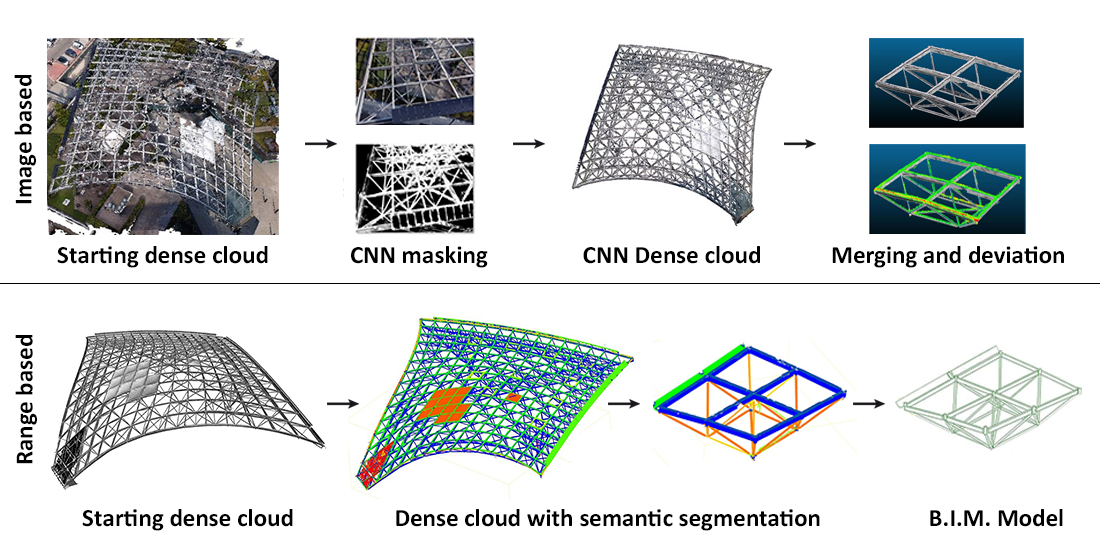
Remotesensing 15 01961 g008
Figure 9. Research process pipeline highlighting the main development steps.
Remotesensing 15 01961 g009
Figure 10. Tree diagram of the structure classification phase.
Remotesensing 15 01961 g010
Figure 11. Photogrammetric blocks divided into eight flight missions.
Remotesensing 15 01961 g011
Figure 12. Workflow for the automated masking of UAV images in photogrammetric processing.
Remotesensing 15 01961 g012
Figure 13. Creation of the training set masks.
Remotesensing 15 01961 g013
Figure 14. Two selected mesh grids for the LoR analysis.
Remotesensing 15 01961 g014
Figure 15. Training set at the first classification level.
Remotesensing 15 01961 g015
Figure 16. Classified point cloud, first level of classification.
Remotesensing 15 01961 g016
Figure 17. Training set and classification results at the second classification level: Classes 12 and 13.
Remotesensing 15 01961 g017
Figure 18. Training set and classification results at the second classification level: Classes 10 and 11.
Remotesensing 15 01961 g018
Figure 19. Training set and classification results at the third classification level: Classes 12 and 13.
Remotesensing 15 01961 g019
Figure 20. Spherical and cylindrical nodes of the TLS point cloud.
Remotesensing 15 01961 g020
Figure 21. Timing comparison between the manual and ML-MR approaches.
Remotesensing 15 01961 g021
Figure 22. Masks resulting from the first attempt.
Remotesensing 15 01961 g022
Figure 23. The most significant masks resulting from the second attempt compared to those from the first attempt; images related to flight 8.
Remotesensing 15 01961 g023
Figure 24. Accuracy and loss graphs for the first training set.
Remotesensing 15 01961 g024
Figure 25. Changing the brightness and contrast of images from the UAV platform.
Remotesensing 15 01961 g025
Figure 26. Masks resulting from the third attempt compared to those from the second attempt. Images related to flight 3.
Remotesensing 15 01961 g026
Figure 27. Masks resulting from the sum of the third attempt with those of the second attempt.
Remotesensing 15 01961 g027
Figure 28. Prediction of the classification on the test set of some flights of all of the attempts made.
Remotesensing 15 01961 g028
Figure 29. From left to right: dense cloud obtained with no prior image masking; dense cloud obtained via CNN-based image masking; dense cloud via the final rectification process.
Remotesensing 15 01961 g029
Figure 30. Comparison between the manual and AI masking times.
Remotesensing 15 01961 g030
Figure 31. Merging of the two total dense clouds from the TLS and RPAS survey.
Remotesensing 15 01961 g031
Figure 32. Deviation analysis on the total dense point cloud between the TLS and RPAS data.
Remotesensing 15 01961 g032
Figure 33. Elements with a high total dense cloud deviation.
Remotesensing 15 01961 g033
Figure 34. The TLS and RPAS merged dense clouds for the two grids, with respective analysis of the deviation and reconstructed mesh.
Remotesensing 15 01961 g034
Figure 35. The mesh reconstruction examples for the classes of rectangular and tubular beams.
Remotesensing 15 01961 g035
Figure 36. Solid geometries built starting from the approximate mesh.
Remotesensing 15 01961 g036
Figure 37. Reconstructed model deviation analysis with respect to the survey data for the first mesh grid.
Remotesensing 15 01961 g037
Figure 38. Classified point cloud and corresponding BIM model for the two selected mesh grids.
Remotesensing 15 01961 g038
Table 1. Classes of reliability identified to evaluate the 3D reconstruction process.
Level of ReliabilityDeviation
High≤10 mm
Medium10 mm < x ≤ 20 mm
Low>20 mm
Table 2. Estimate of the ML-MR classification time via RF for a single classification level (in bold the total time required).
ML-MR Classification via Machine LearningMinutes
1. Creation of the training set120
2. Feature extraction and selection60
3. RF training60
4. Back interpolation30
Total time required270 (4.5 h.)
Table 3. Time required for automated image masking activities (in bold the total time).
AI MaskingMinutesWorking Days *
1. Creation of the training set969521
2. Editing in Lightroom80-
3. Deep learning network training270-
4. Mask rectification135-
Total time required10,18021
* The working day was estimated to be eight hours per day.
Table 4. Comparison of the annotation times between manual masking and AI masking.
Manual masking≈100 working days
(Manual single image annotation ≈ 35 min)
AI masking≈21 working days
Table 5. The LoR evaluation for the first grid, based on deviation from the survey data.
ElementDeviation from Survey Data (mm)Level of Reliability
Rectangular beams10High
Tubular beams4High
Spherical knots13Medium
Cylindrical knots40Low
Gutter15Medium
Disclaimer/Publisher’s Note: The statements, opinions and data contained in all publications are solely those of the individual author(s) and contributor(s) and not of MDPI and/or the editor(s). MDPI and/or the editor(s) disclaim responsibility for any injury to people or property resulting from any ideas, methods, instructions or products referred to in the content.

